| Issue |
A&A
Volume 705, January 2026
|
|
|---|---|---|
| Article Number | A189 | |
| Number of page(s) | 10 | |
| Section | Planets, planetary systems, and small bodies | |
| DOI | https://doi.org/10.1051/0004-6361/202555476 | |
| Published online | 22 January 2026 | |
Boosting decision trees for the selection of main belt asteroids in planetary ephemerides: An alternative model
1
Université Côte d’Azur, Observatoire de la Côte d’Azur, CNRS,
Geoazur, 250 avenue A. Einstein,
06560
Valbonne,
France
2
CRAS, Sapienza University of Rome,
via Eudossiana 18,
00184
Rome,
Italy
3
LTE, Observatoire de Paris, Université PSL, Sorbonne Université, Univ. Lille, Laboratoire National de Métrologie et d’Essai, CNRS,
75014
Paris,
France
★ Corresponding author: This email address is being protected from spambots. You need JavaScript enabled to view it.
; This email address is being protected from spambots. You need JavaScript enabled to view it.
Received:
11
May
2025
Accepted:
27
October
2025
Abstract
Context. One of the main bottlenecks in assessing the accuracy of the Mars orbit is the unknown value of the asteroids in the main asteroid belt. A modeling with 343 asteroids as point masses is used today, with the relative masses fit to observational data.
Aims. We propose an innovative method for reducing the number of asteroids implemented as point masses, which in turn reduces the number of parameters to be fit without a significant degradation of the postfit residuals.
Methods. We used boosting decision trees to obtain a ranking by relative importance of the 343 asteroids of the current main belt modeling.
Results. We were able to remove more than 100 of these asteroids without significantly degrading the postfit residuals and with a significant improvement of the uncertainties. Furthermore, we verified that the postfit masses found with the new modeling (INPOP25c) are consistent with respect to the mass estimation from an independent approach by means of the albedo properties of the asteroids.
Key words: celestial mechanics / ephemerides / minor planets, asteroids: general
© The Authors 2026
 Open Access article, published by EDP Sciences, under the terms of the Creative Commons Attribution License (https://creativecommons.org/licenses/by/4.0), which permits unrestricted use, distribution, and reproduction in any medium, provided the original work is properly cited.
This article is published in open access under the Subscribe to Open model. This email address is being protected from spambots. You need JavaScript enabled to view it. to support open access publication.
1 Introduction
To accurately predict the position of a celestial body in the Solar System is a problem that is rooted in the beginning of astronomy. Over the time, the quantity of observations increased and the quality improved. Several tools for planetary orbitography have been developed so far from different teams around the world. These include the INPOP (Intégrateur Numérique Planétaire de l’Observatoire de Paris) planetary ephemerides (Fienga et al. 2021) that have been developed since 2003, and they are based on the numerical integration of a dynamical model for the planetary orbits that includes several effects: of the relativistic N-body problem considering the eight planets, Pluto, Moon and asteroids (massive asteroids of the main belt are implemented as point-mass perturbers), trans-Neptunian objects (TNOs) (Fienga et al. 2019b; Fienga et al. 2021), and the solar oblateness and Lense-Thirring effect for solar physics (Fienga et al. 2015). Moreover, the Earth-Moon interaction is considered and the lunar interior is taken into account (Viswanathan 2017). In order to fit the parameters of the dynamical model, the least-squares (LS) method is used (Tapley et al. 2004), and the Boundary Value Least-squares (BVLS) method (Lawson & Hanson 1995) is applied to minimize the weighted sum of the residuals. The metric used to assess the goodness of the fit, that is, what we minimize with the BVLS procedure, is the χ2, which we define as
 (1)
where P are the fit parameters,
(1)
where P are the fit parameters,  is the set of observations, gj represents the computation of the observables corresponding to
  , and σj are the observational uncertainties. The χ2 defined with Eq. (1) depends upon some parameters P, and we therefore have the function
 which associates the values of P with the corresponding value of χ2(P). In Eq. (1) we neglected the dependences on time for the sake of simplicity, but we recall that they were taken into account during the χ2 computation.
The question of modeling the Main Asteroid Belt (MAB) perturbations on the inner planet orbits has been addressed since the 1980s (Williams 1984) with the goal of finding a reliable model for many thousands of objects with unknown masses that might have a significant gravitational effect on the inner planets (mainly Mars). Williams (1984) proposed a specific list of 343 individual objects among the Main Belt Asteroids (MBAs) and gathered the most perturbing objects to consider for the construction of accurate planetary ephemerides.
For the highest-mass asteroids, such as (1) Ceres and (4) Vesta, the relativistic contribution is considered next to the Newtonian one (Fienga et al. 2021). In the current MAB modeling of INPOP for the smallest asteroids, instead, only the Newtonian part is accounted in the equations of motion. The orbits of the MBAs are integrated together with the orbits of the planets within a full N-body problem framework, although the mutual interactions among asteroids are not accounted for, except for the five largest, ( (1) Ceres, (2) Pallas, (4) Vesta, (10) Hygieia, and (704) Interamnia).
The range measurements on the Earth-Mars distance are accurate for Mars by about 1 m, whereas the effect of the MBAs on the Mars orbit can reach a few kilometers (Standish & Fienga 2002). When the position of Mars is to be predicted with an uncertainty comparable to the observational accuracy, the asteroid perturbations have to be estimated extremely accurately. We might therefore need a model with an accuracy of 0.1% or even lower. The orbits of the asteroids are usually known, but their masses are not, except for specific cases. Most of the uncertainty is therefore related to the mass, more than to the orbit (Carry 2012; Fienga et al. 2019b; Mariani 2024).
Over the years, several approaches have been developed to address the difficulty of determining which asteroids should be included when modeling their perturbative effects on the planets. One of the earliest attempts to estimate asteroid masses from range observations was presented by Standish & Hellings (1989). A more detailed discussion of the challenges associated with incorporating the masses of MBAs into planetary ephemerides was provided by Standish & Fienga (2002); Fienga & Simon (2004); Kuchynka & Folkner (2013); Fienga et al. (2019b), and can be summarized as follows. The usual approach for determining asteroid masses within planetary ephemerides involves two steps: the asteroid selection, and an adjustment to observations. The asteroid selection identifies the bodies that are to be included in the dynamical model, that is, those with a non-negligible effect on planetary trajectories relative to observational uncertainties. The adjustment step then estimates the corresponding masses. This approach presents two main challenges: (i) systematic errors in mass estimates are difficult to assess because certain asteroids are omitted in the model, and (ii) it is intrinsically challenging to identify perturbing asteroids whose masses remain unknown. The estimation of MBA masses depends on the perturbations they induce on interplanetary distances. In this context, Mars spacecraft tracking provides the most precise range observations because the planet Mars is most strongly perturbed by MBAs due to its proximity. Standish & Hellings (1989) used this method for the first time to determine the masses of (1) Ceres, (2) Pallas, and (4) Vesta from their perturbations on the Mars orbit. Williams (1984) proposed an analytical approach to identify the asteroids that most strongly perturb the orbit of Mars. His study yielded an unpublished list of 300 asteroids that were obtained to support JPL in the orbital solutions of the Solar System by numerical integration (Standish 1998). A new list was derived and used in DE430 Folkner et al. (2014). It considered the physical properties of the asteroids and assessed the effect on the Mars orbit by numerical integration. This increased the list from 300 to 343 asteroids. Kuchynka & Folkner (2013) used a Tikhonov regularization to estimate the asteroid masses in order to deal with the systematic errors for the omission of the asteroids from the modeling. Fienga et al. (2019b) determined the masses of 103 asteroids with uncertainties better than 33% by deducing them in using a Monte Carlo approach for assessing the sensitivity of these determinations, to the boundaries used in the fit. A complementary way to model the Main Belt is to use one (or multiple) solid ring. Krasinsky et al. (2002) proposed a model combining the individual contribution of 300 MBAs, and the contribution from all the remaining small asteroids was modeled as a solid ring in the ecliptic plane, as is adopted in the EPM ephemerides estimation (Pitjeva 2005). In subsequent years, further studies adopting the ring model were Fienga et al. (2009); Kuchynka et al. (2010); Liu et al. (2022).
We describe an innovative method that we used to obtain a ranking by relative importance of the 343 asteroids that are currently used in the MAB modeling for planetary orbitography (Fienga et al. 2021). Starting from this ranking, we provide a reduced list of asteroids whose absence does not degrade the accuracy of the fit significantly. This reduces the number of components of the vector P (of the overall fit) by more than 140 components. To reach this aim, first we used a supervised-learning tool called boosting decision trees (Breiman et al. 1984; Hastie et al. 2009) to obtain the ranking. We then verified the goodness of the ranking fit for the asteroid masses to the full observational dataset using the MAB modeling with a reduced number of asteroids. The ranking plays a key role because it allowed us to test which asteroids might be removed and which were relevant, following their relative importance in terms of gravitational perturbations. The full results are shown in Sect. 2. In Sect. 3 we discuss our results, in particular, the asteroid masses, and we compare them with those from previous versions of INPOP as well as with the EPM2021 planetary ephemerides. In addition, we present a comparison with independent mass estimates obtained through a neural-network albedo algorithm. Finally, in Sect. 3.3, we introduce an innovative method to compare asteroid masses: the Wasserstein barycenter (Villani 2008; Puccetti et al. 2020). This tool is an advanced mathematical concept used to average probability distributions of different origins in a fully consistent way. Given two different distributions (e.g., when the mass of an asteroid is represented as a probability distribution in the Bayesian approach), the Wasserstein barycenter produces a new distribution that represents an average of the two, taking into account the effort required to move one distribution into the other. This effort is measured by the so-called Wasserstein distance, a central concept in optimal transport theory. This approach can be particularly useful in the context of data fusion, for instance, when distributions from different sources are combined. In our case, each probability distribution represents the posterior distribution of the mass of a given MBA.
2 Boosting decision tree for a ranking of asteroids
The aim of machine-learning is to make predictions based on training examples. These techniques have now become an important part of the algorithmic toolbox of a researcher. The goal of this section is to describe the tools of machine-learning we used to select asteroids in the Main Belt: the boosting decision trees (BDT). Among the several machine-learning methods, gradient tree boosting has the great advantage of providing a ranking of the variables in input to the regression function. This aspect, next to increasing the interpretability of the regression itself, plays a key role in our work to obtain a ranking by relative importance of the masses for the 343 asteroids of the MAB modeling, as described above. In this section, we present the main steps of the method. The full algorithm and explanation are given in Mariani (2024).
2.1 Methods. Boosted decision trees for regression
Understanding the gravitational influence of asteroids in the Main Belt is crucial for high-precision solar system dynamics, particularly in spacecraft navigation and ephemeris modeling. This study leverages Boosted Decision Trees (BDT) to rank the 343 asteroids based on their effect on the residuals of Mars Express (MEX) tracking data. The goal is to identify the asteroids that significantly perturb the dynamical model, allowing for targeted refinements in planetary ephemerides.
Decision trees (DT) are a supervised-learning method (Hastie et al. 2009) that partitions the domain into rectangular regions and fits a constant value to each. This partition can be represented, by construction, as a binary tree structure (Mazur 2010). While a single DT provides a piecewise-constant approximation on each region (Breiman et al. 1984; Hastie et al. 2009), the combination of multiple regression trees via boosting (Friedman 2001; Hastie et al. 2009) (sequentially added regression decision trees) improves the predictive accuracy. Each new tree focuses on the residuals (errors) of the previous tree prediction with respect to the values of the training set. This refines the ensemble of trees iteratively. Each DT is built by splitting along one of the axes in the n-dimensional domain of the variables in input for the function that is to be reproduced. Each new rectangle of the partition corresponds to a split along an axis and also to a split in the binary tree representing the partition. The algorithm used for the training (Chen & Guestrin 2016) ranks the input variables (here, asteroid masses) by (i) the frequency of splits for each input variable, that is, how often a variable is used to partition the data and (ii) the improvement in fit induced by this split, characterized by the reduction in prediction error attributed to each new partition region. We used XGBoost (Chen & Guestrin 2016), an optimized gradient-boosting framework that incorporates regularization to prevent overfitting. The implementation details can be found in Chen & Guestrin (2016) and in references therein. In other words, like several tools in the family of supervised-learning methods, a BDT is a way to obtain a regression function over a training set 𝒟. Each instance of the training set in our case represents the known point (x, f∗(x)) ∈ ℝd × ℝ, where f∗ is the target function, that is, the function we would like to reproduce by means of the BDT regression, and d is the number of components of x, the input variables for f∗. In particular, x ∈ ℝd is a vector of size d, whereas f∗(x) ∈ ℝ is a scalar. To define a decision tree (i.e., to obtain a ranking on the input variables of the target function), we therefore need two things: a training set 𝒟, and a target function f*.
2.2 Defining the target function
2.2.1 Preliminary considerations
In this paragraph, we explain the ratio for the objective function we chose, starting from which we built the training set 𝒟. Starting from Eq. (1), we considered the χ2 function as a function of the parameters P ∈ ℝp, meaning that we have ℝp ∋ P ↦ χ2(P) ∈ ℝ. At each iteration of the LS procedure the parameters P are modified by a vector ∆P added to the previous computed parameters. Consequently, a new value of the χ2 is obtained, modified with respect to the previous one by a quantity that we call ∆χ2. Passing from one iteration of the LS to the next, the variation ∆χ2 is a function of the variation ∆P, that is, ℝp ∋ ∆P ↦ ∆χ2(∆P) ∈ ℝ. We considered some components k ∈ ℝp′ of the vector P (then, 1 ≤ p′ ≤ p). If we had a variation ∆k of the only components k, then χ2 also changes by a value ∆χ2 that only depends on the changes in the components k. Therefore, a way to understand the effect of the components k on the computation of the final χ2 is to study the variation ∆χ2 that is only due to ∆k, meaning that we would like to investigate the importance of the variables k on the function given in Eq. (2)
 (2)
(2)
Using Eq. (2), and training a BDT on a properly defined training set 𝒟, we obtained a ranking by construction (and a relative importance) for the components k of P we considered. Moreover, when we already know that k only affects a subset 𝒪∗ of the whole set of observations 𝒪tot strongly, we can restrict ourselves to only consider the ∆χ2 computed on that subset of observations 𝒪∗ ⊆ 𝒪tot. We can then consider a restriction of the function presented in Eq. (2) to the subset 𝒪∗, which we denote by ∆χ2|𝒪∗ : ℝp′ ⟶ ℝ. This function maps variations in certain variables k of P to the corresponding variations in χ2, restricted to its value computed using the observations in the subset 𝒪∗ alone. Following the notation in Eq. (2), we rewrite this as
 (3)
(3)
We emphasize that what we have described so far applies to a χ2 computed using a full dynamical model of the Solar System (see, e.g., Eq. (1)). Our approach was to use as the target function for the BDT construction the quantity expressed in Eq. (2), with k = mAST representing the components of P corresponding to the 343 MBA masses fit in INPOP. We obtained a ranking for the components of mAST ∈ ℝ343, that is, the point-mass asteroids in the MAB modeled in INPOP. Therefore, Eq. (3) becomes
 (4)
(4)
Starting from this ranking, provided by the BDT, we can remove the least important asteroids in order to improve the dynamical modeling. For the notation, by mAST ∈ ℝ343 we denote the vector of the masses for the asteroids modeled in the dynamical system we considered, whereas ∆mAST ∈ ℝ343 has to be interpreted as a variation in the mass value that affects the χ2 by a certain ∆χ2 (see, e.g., Eq. (3)). In order to produce an effective training set 𝒟, we used as the target function an approximate form of Eq. (4), obtained by linearizing the residuals (O − C) as explained in the following paragraph.
2.2.2 The target function and training set
The strategy consists of reproducing a target function f∗ = f∗(∆mAST), function of the asteroid masses, using a BDT. As a consequence, the ranking of the masses mAST is obtained, based on the relative importance for each one of the components of mAST. Through the BDT, it is possible to know the relative importance for each component of mAST in reproducing f∗. The f∗ we chose quantifies the effect of changes in asteroid masses ∆mAST on the goodness-of-fit metric χ2, as defined in Eq. (1). Following the approach described up to Eq. (3), we chose as the target function f∗ an approximate form of Eq. (4), where the considered subset of observations consists of MEX tracking residuals. For simplicity, we denote this 𝒪∗ = 𝒪MEX.
For the sake of computational efficiency (see the discussion in Mariani 2024), we approximated χ2 with a quadratic expression with respect to ∆mAST, resulting in a target f∗ of
 (5)
(5)
In Eq. (5),  is the approximate change in χ2 induced by a change in the masses ∆mAST, whereas 𝒪MEX denotes the hypothesis of restricting χ2 to the MEX spacecraft observations. The slightly different notation introduced in Eq. (5) emphasizes the computation of
  with an approximate form, as detailed below.
For each perturbation  , we then computed the corresponding
  using linearized residuals,
![Mathematical equation: ${\rm{\Delta }}\tilde \chi _O^2({\rm{\Delta }}{m^{{\rm{AST}}}}) = {[{\rm{\Delta }}(\widetilde {O - C}){|_O}]^T}[{\rm{\Delta }}(\widetilde {O - C}){|_O}],$](/articles/aa/full_html/2026/01/aa55476-25/aa55476-25-eq13.png) (6)
where 𝒪 = 𝒪MEX, and
(6)
where 𝒪 = 𝒪MEX, and
![Mathematical equation: ${\rm{\Delta }}(\widetilde {O - C}){|_O}\left. \equiv \right|\left[ {{{\partial (O - C){|_O}} \over {\partial {m^{{\rm{AST}}}}}}} \right]{\rm{\Delta }}{m^{{\rm{AST}}}}$](/articles/aa/full_html/2026/01/aa55476-25/aa55476-25-eq14.png) (7)
is the estimated change in the MEX tracking residuals. The linearity expressed in Eq. (7) is an assumption, as is the restriction to the MEX data. The validity of these assumptions is to be proved by the results presented in Sect. 2.5. Finally, then, the training set
(7)
is the estimated change in the MEX tracking residuals. The linearity expressed in Eq. (7) is an assumption, as is the restriction to the MEX data. The validity of these assumptions is to be proved by the results presented in Sect. 2.5. Finally, then, the training set  links the mass changes to their dynamical effect. In the left side of Eq. (7), we dropped the dependence of
  for simplicity of notation, but we recall that the left sides in Eqs. (6) and (7) both depend upon the ∆mAST that is used to compute them. The matrix of partials used in Eq. (7) is the block of matrix of partials used in the INPOP LS procedure, where the columns considered are those relative to the 343 point-mass asteroids that are fit, whereas the rows are relative to the MEX observations (we refer to Fienga et al. 2021 and references therein for further details about the construction by numerical differences of the matrix of partials used in INPOP). In the left side of Eq. (7), we did not use the actual MEX observations, but computed the full variation in (O − C) by mean of matrix vector multiplication, where ∆mAST is a vector produced randomly to generate the training set. The actual observations and the Solar System dynamics are involved in the matrix of partials used in Eq. (7). The training set we need to generate then is
 (8)
where in Eq. (8)
(8)
where in Eq. (8)  , and M is the size of the training set, whereas i denotes the ith element of the training set 𝒟. The mass variations
  were generated randomly with a uniform distributions within ∼10% of the postfit values from the INPOP21a ephemerides model (Fienga et al. 2021). In light of the preceding discussion, the assumption of using a ∼10% mass variation to generate the masses
  for the training set is justified by the necessity to remain in the linear regime such that Eq. (7) might hold. Moreover, in this first phase of the study, the goal was not to obtain the mass values (they are obtained below with the fit), but to investigate by means of the training set the sensitivity to the masses in the linear regime, which is a key assumption here.
The BDT model processes 𝒟 to assign an importance score to each asteroid that reflects its influence on MEX residuals. The importance is relative to that of other asteroids and to the specific datasets used (𝒪MEX, i.e., range measurements from MEX mission). The limitation of this approach is mainly in the linearized residual of the Eq. (7) approximation that might miss nonlinear effects; future work might consider full numerical simulations to produce the training set.
2.3 Improving the planetary ephemerides
To implement the ranking established with the BDT, we started from an updated version of INPOP planetary ephemerides that we call INPOP25a. This version was built using the same procedure as for INPOP21a (Fienga et al. 2021), but the adjustment interval was prolonged from 2019 to 2022. Compared to previous releases, INPOP25a incorporates an extended time span of Juno and MEX range data, as well as newly added Juno VLBA astrometric measurements. Fienga et al. (2019b) reported that the current limitation of planetary ephemerides is mainly their capability of extrapolation for the Mars geocentric distances.
Fienga et al. (2019b) proposed that the most recent knowledge of asteroid bulk densities should be taken into account using a random Monte Carlo sampling of the boundaries that are used to construct the planetary ephemeris. INPOP19a, INPOP21a, and the most recent INPOP25a were built using this procedure and kept the same boundaries as issued by Fienga et al. (2019b). Fig. 1 clearly shows, however, that the issue of the extrapolation is still present. To improve this, it was decided to relax the boundary conditions by 25% as a way to limit the overconstraint imposed on the adjustment, which might explain the poor extrapolation capability of the model. With the newly obtained ephemeris fit on the same data sample as INPOP25a, we obtained the results we present in the bottom plot of Fig. 1, which indicates a clear improvement of the extrapolation of the new solution (INPOP25b). The improvement affects not only the dispersion of the residuals, but also their general distributions: The new INPOP25b produces an almost normal distribution, whereas the INPOP25a distribution seems to be composed of several multiple distributions, which indicates remaining signals. A small offset is still present, but can be explained by the MEX transponder delay, which was not fit when the extrapolated residuals were computed. As a consequence, we implemented the new asteroid ranking starting from the INPOP25b version for the remainder of this study.
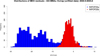 |
Fig. 1 Residual distributions for the extrapolation period using the original boundary interval (in blue) and the extended boundaries (in red). |
2.4 Ranking
As explained in Sects. 2.2.2 and 2.2, the idea was to use a BDT for the regression of a training set 𝒟, as defined in Eq. (8), from which we obtained a ranking of the variables in input to the function f∗ of Eq. (5). As a byproduct, we obtained the relative importance (and the ranking) of the components in ∆mAST, representing the asteroid masses. We produced several training sets, all of them defined through Eqs. (8) and (6), using different sizes (i.e., different M in Eq. (8)) and different hyperparameter configurations for the trees. Fig. 2 only shows the outcome of the solution we obtained with M = 2 × 10⁶, which is the best result we found so far. The relative variable importance is provided in a way such that the sum of them, for all the asteroids, is one. Therefore, it is easy to interpret the importance for each asteroid as a percentage with respect to the global importance. Fig. 2 shows that more than 80% of the global importance derives from just three asteroids: (1) Ceres, (2) Pallas, and (4) Vesta with importances between 20 and 30%. Following them, with an importance between 1 and 5% we find (3) Juno, (324) Bamberga, (10) Hygiea, and (19) Fortuna. Subsequently, only asteroids with a relative importance below 1% were found. This first computation already shows that most asteroids have a small relative importance alone, but their importance is not negligible when all are considered together. This first outcome also confirms the very widespread correlation among the asteroids in the planetary orbitography fit, as already pointed out by Kuchynka & Folkner (2013); Fienga et al. (2019b) and Mariani (2024). In other words, the effect of the ensemble of asteroids is not negligible. To obtain a clear assessment of the ranking, however, we need to use it with the full fit of planetary ephemerides. In Sect. 2.5 we introduce the ranking in the fit to improve the dynamical model.
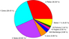 |
Fig. 2 Pie chart of the relative importance for the first asteroids in the ranking obtained with 2 × 10⁶ elements. |
2.5 Introducing the fit ranking
The ranking obtained with the BDT provides relevant information about the importance of each asteroid in the global reconstruction of the Earth-Mars distances as deduced from the MEX navigation data. The point then is to determine how effective this ranking is when the global construction of the whole planet orbitography is to be considered. To do this, we started from one initial planetary ephemeris and removed the asteroids following the BDT ranking one by one, starting from the least important objects. By removing the asteroid, we mean that we no longer considered the object in the dynamical modeling, and we consequently did not estimate its mass in the global planetary fit. We built a full ephemeris by removing the considered objects and by iteratively fitting the obtained integration. For the fit, we did not only consider the MEX tracking data, but we adjusted the eight planets in the Solar System using the complete set of available observations. We used the INPOP25a datasets. We removed the asteroids by accumulation, meaning that for the first removed object, the integration counted 342 asteroids, and when the asteroid ranked 200 in the BDT list was removed, 143 asteroids perturbed the planet orbits. Convergence was obtained before the ninth iteration, and the results of the fit ephemerides in terms of standard deviations of the MEX residuals σMEX and in the global χ2 are shown in Fig. 3.
Fig. 3 allows us to draw several conclusions. The evolution of σMEX and of the global χ2 follows very similar trends, meaning that MEX is indeed a good proxy of the quality of the global ephemerides. The ranking is validated by the increasing differences to the reference solution (INPOP25b) with increasing ranking.
Fig. 3 mainly shows two regimes: in the first regime, asteroids were removed, and this therefore presents the lowest importance according to the BDT. It indeed induced very small differences (below 20 cm) in σMEX and the global χ2. After some limit (up to rank 200), the differences start to increase more strongly, almost with an exponential trend. Fig. 3 shows that removing up to 200 asteroids yields an oscillations in the postfit σMEX lower than 20 cm.
The residual indicator and selection. In order to propose a new solution of planetary ephemerides with an optimized number of perturbing MBAs modeled in the main belt, but without degrading the postfit residuals, next to σMEX and χ2, also the extrapolation capability of the solution found can be taken into account. In order to this, we computed an averaged index that we call residual indicator RI for the several cases we analyzed. RI takes σMEX on the observations used in the fit (σMEX,fit) and the dispersion of the residuals from extrapolation of MEX unfit data (σMEX,ext) into account. RI is defined as  , and it was computed by removing the asteroids in a cumulative way, starting from the least important. Computing the RI for different training sets 𝒟 allowed us to assess the solution that was the best compromise among the number of removed asteroids, postfit σMEX, and extrapolation capability on unfit data. The minimum of RI provides what we consider the best solution, and we call it INPOP25c. The results are shown in Fig. 4. By removing more than 100 asteroids, we propose a solution at 147 removed asteroids, which we obtained from the ranking with M = 2 × 10⁶ elements. The left panel of Fig. 4 shows three different sizes of training sets with M = 5 × 10⁵, M = 2 × 10⁶ or M = 6 × 10⁶. The right panel of Fig. 4 zooms in on the left panel for the best solution.
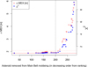 |
Fig. 3 Standard deviation (σMEX) of the MEX residuals in meters and global χ2 obtained with the model without X asteroids. X is given by the x-axis according to the ranking given in Sect. 2.4. The dotted line represents a reference of 20 cm increase relative to INPOP25b σMEX plotted with the full red line. |
3 Discussion and conclusion
We showed that we approximately reproduced and even improved upon the extrapolation of INPOP25a and INPOP25b with INPOP25c and significantly fewer asteroids, especially when the bounds on the masses were relaxed. This naturally raises the question about whether these new masses are physically reasonable.
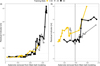 |
Fig. 4 Residual indicator obtained by taking the σMEX,fit obtained after the fit and the σMEX,ext obtained by the extrapolation interval for different sizes of the training sets into account. Panel b shows an enlargement of panel a. The vertical gray line indicates the minimum reached by the residual indicator RI. The corresponding solution also maximizes the number of asteroids we removed from the original main belt selection. The different curves correspond to results obtained starting from training sets of different sizes, as indicated by the legend at the top (half a million, two millions, and six millions). |
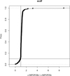 |
Fig. 5 Cumulative histogram of the ratio σ25b over σ25c for the 193 asteroid masses fit in INPOP25b and INPOP25c. |
3.1 Comparisons between INPOP versions
In order to assess the advantages of reducing the number of asteroids from the point of view of asteroid mass determination, we compared the uncertainties on the fit masses obtained with INPOP25b (σ25b) and with INPOP25c (σ25c) for the common masses. Fig. 5 shows the cumulative histogram (empirical cumulative distribution function) of the ratio of σ25b and σ25c for the 196 masses that were fit by INPOP25b and INPOP25c. The uncertainties obtained with INPOP25b for 90% of the objects are larger than the uncertainty obtained with INPOP25c. The improvement induced by the reduced number of fit asteroids in INPOP25c is about 15% on averge compared to INPOP25b. This improvement can be explained by a better conditioning of the Jacobian matrix of the fit with a reduction of 70% of the conditioning number between INPOP25b and INPOP25c. The decrease in the conditioning number is likely due to the smaller set of asteroids that is taken into account during the fit of INPOP25c with respect to INPOP25b. In terms of individual improvements, for 10 masses, the mass uncertainties decrease by more than 50%, and for 32 masses, the decrease is better than 25%. All the masses together with their uncertainties are given in Table A.1. The improvement brought by the reduced number of asteroids in the fit is clearly visible in terms of mass uncertainties and quality of the fit. Furthermore, the choice of INPOP25c was also made for a good trade-off between postfit residuals and extrapolation, as discussed in Sect. 2.5. Finally, it is interesting to note that with fewer asteroids in the dynamical modeling compared to the INPOP25b integration, our approach reduced the computation time by approximately 52% in user time (i.e., time spent in user mode within the process) and by 30% in real time (i.e., the total elapsed time from process initiation to completion).
More globally, we compare the posterior distributions of masses obtained with INPOP19a (Fienga et al. 2019a), INPOP21a (Fienga et al. 2021), INPOP25b, and INPOP25c in panel a of Fig. 6. These plots show that the INPOP mass distributions are quite similar from one ephemeris to the next. It is interesting to note, however, that INPOP19a tends to give lower masses, and with ephemerides involved with more data and progress in the modeling, the dispersion in the mass distribution is reduced. The differences in the mass distributions are stronger between the other determinations, as explained in Sect. 3.2.2.
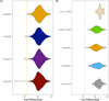 |
Fig. 6 Histograms of the asteroid masses in common to INPOP25b, INPOP25c, INPOP21a (Fienga et al. 2021), INPOP19a (Fienga et al. 2019a), EPM2021 (Pitjeva et al. 2019), Li et al. (2023), Kretlow (2020), and Carry (2012). |
3.2 Comparison with independent mass estimations
3.2.1 Neural-network albedo algorithm
To assess whether the masses obtained with INPOP25c are physically reasonable, we required an independent posterior of the asteroid masses. We generated this posterior by using the neural-network catalog of albedo predictions presented by Murray (2023). This approach uses an ensemble of neural networks to predict the visible albedo of an asteroid and its uncertainty as a function of its proper orbital elements. With the predicted albedo from this catalog (p) and the total uncertainty  , we generated a distribution for the albedo for our objects. We note that four cases had no proper elements: MPC (132) Aethra, (433) Eros, and (1036) Ganymed. In these cases, the albedo was assumed to be as in a log-uniform distribution between 0.01 and 1.0.
These distributions in albedo were then converted into distributions with diameters using the H magnitudes provided by the Minor Planet Center. Finally, a posterior distribution in mass was obtained by assuming that the density was a uniform distribution between 0.5 and 4.5 g/cm3.
To test whether our values were extreme, we considered the distribution of the percentile scores of each of our fit masses with respect to the corresponding posterior distributions. If the generated posterior distributions are the real distributions, the distribution of the posterior scores should be a uniform distribution. If the fit masses are too constrained (or the distributions too wide), they are disproportionally found near the 50th percentile. In the opposite case, they are found disproportionally at the zeroth or 100th percentile.
To test a set of asteroids against each other, we preformed a Kolmogorov-Smirnov test on the resulting percentile distribution and verified its proximity to a uniform distribution. The closer the proximity, the more likely are the fit masses consistent with the posterior distribution. We show a summary of the ECDF (empirical cumulative distribution function) of these distributions in Fig. 7. While all of our distributions are slightly centrally concentrated, likely owing to the wide distributions of densities we considered, there is little difference between the selection of asteroids in this work and those in previous INPOP versions. This suggests that the masses we found are physically reasonable compared to these studies.
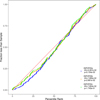 |
Fig. 7 Comparison of the ECDF of the percentile score distribution of our fit masses with respect to the posterior mass distributions. Perfect agreement is denoted by the diagonal red line. We also provide the p values for our tests to assess the statistical significance of our comparisons. |
3.2.2 Comparisons with the literature
We compared the masses issued from the metadata analysis from Carry (2012) and the recent update by Kretlow (2020) and from the close-encounters analysis using Gaia data by Li et al. (2023). The complexity of providing a consistent and homogeneous database for masses comes from the difficulty of associating mass determinations obtained with different methods (planetary ephemerides, binary system, and asteroid-asteroid close-encounters) that are more or less affected by different sources of uncertainties and biases. On one hand, Carry (2012) addressed this issue by using an iterative weighted estimation of the mass and rejected outliers by comparison to the mean and σ values. They also considered estimations without published uncertainties. On the other hand, Kretlow (2020) added supplementary mass determinations compared to Carry (2012) and used more sophisticated statistical estimators (EVM) that are expected to be less sensitive to outliers and provide asymmetric uncertainties (Birch & Singh 2014). Li et al. (2023) reported 20 masses that were obtained from close encounters observed with Gaia DR3 and ground-based observations.
A first global comparison is possible with panel b in Fig. 6. This panel shows the mass distributions in common to INPOP25c, Carry (2012), Kretlow (2020), and Li et al. (2023). The distributions from INPOP25c and Kretlow (2020) are clearly very similar: the same number of objects is obtained with the two distributions. Carry (2012) seems to indicate higher masses than the two former, but with 30% fewer objects. Li et al. (2023) also reported higher masses than Kretlow (2020) and INPOP25c, but this might also be related to the method (close encounters favor higher-mass objects) and the limited number of masses (21) provided by Li et al. (2023). The comparison of the global distribution is affected by the distribution of the asteroid sizes. This is also visible in Fig. 8 in panels A and B. We show 2D histograms of the radii (on the y-axis) and of the ratio of the Kretlow (2020) and INPOP25c masses (panel A) and of the Carry (2012) and INPOP25c masses (panel B). The mean of the asteroid radii in common for Kretlow (2020) and INPOP25c is about 64 km, but it is about 8% higher for Carry (2012) and INPOP25c. Furthermore, Fig. 8 also shows that for asteroids with radii greater than 70 km, the masses are consistent, with a ratio close to one in panels C and D or close to zero in log10 scale in panels A and B.
For smaller objects, however, the discrepancy in masses increases. For the comparison of Kretlow (2020) versus INPOP25c (panels A and C in Fig. 8), the departure from unity is balanced between under- and overestimated INPOP25c masses, with a small bias toward underestimated INPOP25c. A slight departure for asteroids with a radius larger than 100 km is also visible, for which the Kretlow (2020) masses seem to be lower than INPOP25c. This dispersion can be explained by the high uncertainties of the Kretlow (2020) determinations (see panel C of Fig. 8). For the comparison of Carry (2012) versus INPOP25c (panels B and D in Fig. 8), there is a clear bias, with Carry (2012) being systematically larger than INPOP25c for asteroids with radii smaller than 70 km. In contrast to the comparison with Kretlow (2020), however, this bias between Carry (2012) and INPOP25c cannot be explained by uncertainties, as shown in panel D. In conclusion, systematic differences are visible as expected between INPOP25C, Kretlow (2020), and Carry (2012), but INPOP25C and Kretlow (2020) also agree better.
Finally, we compared our solution with asteroid masses obtained by the EPM2021 planetary ephemerides (Pitjeva et al. 2019). Following the Tikhonov regularization proposed by Kuchynka & Folkner (2013), EPM2021 considered 277 asteroids with positive fit masses and 2 asteroid rings located at 2.2 and 3.0 au, for which one mass was adjusted. Fig. 6 shows the distribution of EPM2021 141 masses in common with INPOP25c. In comparison to the INPOP25c and Kretlow (2020) distributions, EPM2021 seems to have a similar distribution with a flatter and bimodal profile with a more abrupt cut for masses lower than 1017 kg. This might be explained by the introduction in EPM2021 of an asteroid ring than was able to reproduce the effect of small objects. Fig. 8 shows that the masses of INPOP25c and EPM2021 agree well inside the 1σ interval, even for small objects. the departure between INPOP25c and EPM2021 masses is slightly larger than between INPOP25c and Kretlow (2020) masses. This is particularly visible in panels A and C, where a small peak of mass ratio around 0.6 is present in panel C for objects with a radius of 60–70 km, where no stiff peak is present in panel A.
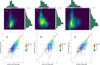 |
Fig. 8 Comparisons between INPOP25c, Carry (2012), Kretlow (2020), and Pitjeva et al. (2019). Panels A–C show the 2D histograms of the radii in kilometers and ratio Kretlow (2020)/INPOP25c (A), the ratio Carry (2012)/INPOP25c (B), and the ratio Pitjeva et al. (2019)/INPOP25c (C). Panels D, E, and F show the masses of INPOP25c vs. the Kretlow (2020) masses (C), masses of INPOP25c vs. Carry (2012) (D), and vs. Pitjeva et al. (2019) masses in panel (F). The color indicates the radii in kilometers. |
3.3 Combining determinations: Wasserstein tools
Finally, we directly compared the probability distribution for the value of each MBA found with this method (Murray 2023) and the postfit masses obtained for INPOP25c, that is, the optimal planetary solution with fewer asteroids. To compare these distributions with those from other sources, we propose an innovative approach from the theory of optimal transport and calculus of variation (Villani 2008; Figalli & Glaudo 2023), specifically, the computational adaptation of the Wasserstein barycenters by means of the package waspr (Cremers 2020) based on the work of Puccetti et al. (2020). The Wasserstein barycenter is a method for averaging two (or more) generic probability distributions in the space of probability distributions, which we applied to the asteroid mass distributions. The Wasserstein barycenter, in particular, does not require that the distributions have the same support (as in the case of the KL divergence) or a specific law explicit in analytical formulation. It can therefore be applied when the same physical quantity in the same unit is considered. The underlying idea is to find a way to merge the information contained in several different posterior distributions available for each asteroid considered in INPOP25c, and to join them using a consistent probabilistic approach, and without making any hypothesis about the law followed by the distribution. This merging is especially important for small asteroids, whose mass estimates can differ significantly between studies. Consequently, the Wasserstein barycenter1 is therefore not a single value, but a probability distribution. For a wider introduction to the topic of computational optimal transport, we refer to Peyré & Cuturi (2020) and references therein. The interest in using the Wasserstein barycenters plays a role within the context of the comparison shown in Sect. 3.2.2. As already pointed out in Sects. 3.1 and 3.2.2, for smaller asteroids, the difference in their mass estimations are larger in the different studies. Using the barycenters, we propose a way to join the information (including their uncertainties) and methods of the previous investigations together with the mass determinations found during the fit procedure of INPOP25c. In Table A.1 we report the masses found with INPOP25c and the mean of the Wasserstein barycenters. The Wasserstein barycenters were computed between the normal distributions obtained with INPOP25c, the posterior distributions obtained using albedos and neural networks (Murray 2023), and those with the normal distributions proposed by Kretlow (2020). We show here some specific examples to illustrate the use of the Wasserstein barycenter, in particular, we show in Fig. 9 the case of the mass of (20) Massalia, and in Fig. 10 we show the mass of (28) Bellona. In the case of (20) Massalia, Fig. 9 shows that the estimates from INPOP25c and Kretlow (2020) both have a small uncertainty (σ), and within the uncertainty of the albedo estimate, however, the two normal distributions differ. In this case, the Wasserstein barycenter provides an intermediate estimate among the three cases. For (28) Bellona, the example of a Wasserstein barycenter is not a normal distribution, but more similar to a log-normal distribution. This shows the flexibility and generality of the tool that might handle different types of uncertainties and distributions simultaneously. Furthermore, Fig. 11 shows the several distributions involved in the computation of the barycenter for (20) Massalia, panel (a) and 28 Bellona, panel (b), visualized as disentangled distributions to stress their differences even for the same asteroid. We point out, however, that the mean and standard deviation obtained from the computation of the barycenters is not intended as a better estimate of what has been found with previous mass determinations. On the other hand, it is a tool that might be used for specific cases of asteroids for which the information is poor and the different estimates differ. For these, it might become a way to unify them in a probabilistic approach.
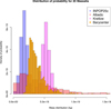 |
Fig. 9 Histograms of the mass distributions for (20) Massalia estimated from INPOP25c, neural networks, and albedo (Sect. 3.2.1 and Murray 2023 and Kretlow 2020). The Wasserstein barycenter resulting from the three posteriors cited is shown in yellow. |
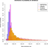 |
Fig. 10 Histograms of the mass distributions for (28) Bellona estimated from INPOP25c, neural networks, and albedo (Sect. 3.2.1 and Murray 2023 and Kretlow 2020). The Wasserstein barycenter resulting from the three posteriors cited is shown in yellow. |
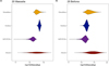 |
Fig. 11 Histograms of the mass distributions for (28) Bellona estimated from INPOP25c, neural networks and albedo (Sect. 3.2.1 and Murray 2023 and Kretlow 2020). The Wasserstein barycenter resulting from the three posteriors cited is shown in yellow. |
4 Conclusions
We have presented the use of boosting decision trees in order to obtain a ranking by relative importance of the point-mass modeling for the main belt asteroids used in INPOP. Starting from this list of asteroids, we were able to remove more than 100 asteroids without significantly degrading the postfit residuals and with a significant improvement of the uncertainties . Moreover, we verified that the postfit masses found with the new modeling (INPOP25c) were consistent with respect to the mass estimate found with an independent and different approach by means of the albedo properties of the asteroids. Finally, we proposed a comprehensive comparison with mass estimates in the literature using different statistical tools. Using the Wasserstein barycenter, we finally merged different asteroid mass estimates and showed that this innovative approach might help in specific cases for poorly determined masses. In the future, the technique proposed by boosting decision trees can help us to improve dynamical modeling within the Solar System, such as for TNOs, although computational issues must be addressed in advance and must be solved.
Data availability
Supplementary material in electronic format (ASCII tables) is available at the CDS via https://cdsarc.cds.unistra.fr/viz-bin/cat/J/A+A/705/A189. The file Table_A1.dat (in the text, Table A.1) provides the list of the asteroid masses obtained in INPOP25c. In the first, second and third column we show respectively the postfit mass, 1σ uncertainty and noise-to-signal ratio found with INPOP25c adjustment to observations. In the fourth and fifth column we present respectively the mean and standard deviation of the Wasserstein barycenters obtained as described in Sect. 3.2.2. The last column indicates the ranking position of each asteroid. The file Table_A2.dat contains the ranking positions of the 343 asteroids modeled as point masses in INPOP21a: the first column gives the ranking position, and the second column lists the MPC number of each asteroid.
Acknowledgements
This work was supported by the French government through the France 2030 investment plan managed by the National Research Agency (ANR), as part of the Initiative of Excellence Université Côte d’Azur under reference number ANR-15-IDEX-01. The authors are grateful to the Université Côte d’Azur’s Center for High-Performance Computing (OPAL infrastructure) for providing resources and support. This work was supported by CNES (French Space Agency) and Université Côte d’Azur with EUR-SPECTRUM Consortium. V.M. thanks Alberto Perrella for the fruitful discussions about optimal transport theory. This research was conducted while V.M. was at the Observatoire de la Côte d’Azur; V.M. is currently at Sapienza University of Rome.
References
- Birch, M., & Singh, B. 2014, Nucl. Data Sheets, 120, 106 [NASA ADS] [CrossRef] [Google Scholar]
- Breiman, L., Friedman, J., Stone, C. J., & Olshen, R. 1984, Classification and Regression Trees (London: Chapman and Hall/CRC) [Google Scholar]
- Carry, B. 2012, Planet. Space Sci., 73, 98 [CrossRef] [Google Scholar]
- Chen, T., & Guestrin, C. 2016, arXiv e-prints [arXiv:1603.02754] [Google Scholar]
- Cremers, J. 2020, waspr: Wasserstein Barycenters of Subset Posteriors [Google Scholar]
- Fienga, A., & Simon, J.-L. 2004, A&A, 429, 361 [Google Scholar]
- Fienga, A., Laskar, J., Morley, T., et al. 2009, A&A, 507, 1675 [NASA ADS] [CrossRef] [EDP Sciences] [Google Scholar]
- Fienga, A., Laskar, J., Exertier, P., Manche, H., & Gastineau, M. 2015, Celest. Mech. Dyn. Astron., 123, 325 [Google Scholar]
- Fienga, A., Deram, P., Viswanathan, V., et al. 2019a, Notes Scientifiques et Techniques de l’Institut de Mecanique Celeste, 109 [Google Scholar]
- Fienga, A., Avdellidou, C., & Hanuš, J. 2019b, MNRAS, 492, 589 [Google Scholar]
- Fienga, A., Deram, P., Di Ruscio, A., et al. 2021, Notes Scientifiques et Techniques de l’Institut de Mecanique Celeste, 110 [Google Scholar]
- Figalli, A., & Glaudo, F. 2023, An Invitation to Optimal Transport, Wasserstein Distances, and Gradient Flows, 2nd edn. (Berlin: European Mathematical Society) [Google Scholar]
- Folkner, W. M., Williams, J. G., Boggs, D. H., Park, R. S., & Kuchynka, P. 2014, Interplanet. Netw. Prog. Rep., 196, 1 [Google Scholar]
- Friedman, J. H. 2001, Annal. Stat., 29, 1189 [CrossRef] [Google Scholar]
- Hastie, T., Tibshirani, R., & Friedman, J. 2009, The Elements of Statistical Learning: Data Mining, Inference, and Prediction, 2nd edn. (Berlin: Springer Series in Statistics) [Google Scholar]
- Krasinsky, G., Pitjeva, E., Vasilyev, M., & Yagudina, E. 2002, Icarus, 158, 98 [CrossRef] [Google Scholar]
- Kretlow, M. 2020, Euro. Planet. Sci. Cong., EPSC2020, 690 [Google Scholar]
- Kuchynka, P., & Folkner, W. M. 2013, Icarus, 222, 243 [NASA ADS] [CrossRef] [Google Scholar]
- Kuchynka, P., Laskar, J., Fienga, A., & Manche, H. 2010, A&A, 514, A96 [NASA ADS] [CrossRef] [EDP Sciences] [Google Scholar]
- Lawson, C. L., & Hanson, R. J. 1995, Solving Least Squares Problems (Philadelphia: Society for Industrial and Applied Mathematics) [Google Scholar]
- Li, F., Yuan, Y., Fu, Y., & Chen, J. 2023, AJ, 166, 93 [Google Scholar]
- Liu, S., Fienga, A., & Yan, J. 2022, Icarus, 376, 114845 [Google Scholar]
- Mariani, V. 2024, PhD thesis, Observatoire de la Côte d’Azur, France [Google Scholar]
- Mazur, D. 2010, Combinatorics: A Guided Tour, MAA textbooks (USA: Mathematical Association of America) [Google Scholar]
- Murray, Z. 2023, PSJ, 4, 90 [Google Scholar]
- Peyré, G., & Cuturi, M. 2020, Computational Optimal Transport (Norwell: Now publishers) [Google Scholar]
- Pitjeva, E. V. 2005, Sol. Syst. Res., 39, 176 [Google Scholar]
- Pitjeva, E., Pavlov, D., Aksim, D., & Kan, M. 2019, Proc. Int. Astron. Union, 15, 220 [Google Scholar]
- Puccetti, G., Rüschendorf, L., & Vanduffel, S. 2020, J. Multiv. Anal., 176, 104581 [Google Scholar]
- Standish, E. M. J. 1998, JPL IOM, 312.F-98-048 [Google Scholar]
- Standish, E., & Hellings, R. W. 1989, Icarus, 80, 326 [NASA ADS] [CrossRef] [Google Scholar]
- Standish, E. M., & Fienga, A. 2002, A&A, 384, 322 [NASA ADS] [CrossRef] [EDP Sciences] [Google Scholar]
- Tapley, B., Schutz, B., & Born, G. 2004, Statistical Orbit Determination, 1st edn. (Amsterdam: Elsevier) [Google Scholar]
- Villani, C. 2008, Optimal Transport: Old and New, Grundlehren der mathematischen Wissenschaften (Berlin Heidelberg: Springer) [Google Scholar]
- Viswanathan, V. 2017, PhD thesis, France [Google Scholar]
- Williams, J. 1984, Icarus, 57, 1 [Google Scholar]
The reader should note that we use this tool since it allows a fully consistent comparison among probability distributions of whatever shape and support.
All Figures
|
Fig. 1 Residual distributions for the extrapolation period using the original boundary interval (in blue) and the extended boundaries (in red). |
| In the text | |
|
Fig. 2 Pie chart of the relative importance for the first asteroids in the ranking obtained with 2 × 10⁶ elements. |
| In the text | |
|
Fig. 3 Standard deviation (σMEX) of the MEX residuals in meters and global χ2 obtained with the model without X asteroids. X is given by the x-axis according to the ranking given in Sect. 2.4. The dotted line represents a reference of 20 cm increase relative to INPOP25b σMEX plotted with the full red line. |
| In the text | |
|
Fig. 4 Residual indicator obtained by taking the σMEX,fit obtained after the fit and the σMEX,ext obtained by the extrapolation interval for different sizes of the training sets into account. Panel b shows an enlargement of panel a. The vertical gray line indicates the minimum reached by the residual indicator RI. The corresponding solution also maximizes the number of asteroids we removed from the original main belt selection. The different curves correspond to results obtained starting from training sets of different sizes, as indicated by the legend at the top (half a million, two millions, and six millions). |
| In the text | |
|
Fig. 5 Cumulative histogram of the ratio σ25b over σ25c for the 193 asteroid masses fit in INPOP25b and INPOP25c. |
| In the text | |
|
Fig. 6 Histograms of the asteroid masses in common to INPOP25b, INPOP25c, INPOP21a (Fienga et al. 2021), INPOP19a (Fienga et al. 2019a), EPM2021 (Pitjeva et al. 2019), Li et al. (2023), Kretlow (2020), and Carry (2012). |
| In the text | |
|
Fig. 7 Comparison of the ECDF of the percentile score distribution of our fit masses with respect to the posterior mass distributions. Perfect agreement is denoted by the diagonal red line. We also provide the p values for our tests to assess the statistical significance of our comparisons. |
| In the text | |
|
Fig. 8 Comparisons between INPOP25c, Carry (2012), Kretlow (2020), and Pitjeva et al. (2019). Panels A–C show the 2D histograms of the radii in kilometers and ratio Kretlow (2020)/INPOP25c (A), the ratio Carry (2012)/INPOP25c (B), and the ratio Pitjeva et al. (2019)/INPOP25c (C). Panels D, E, and F show the masses of INPOP25c vs. the Kretlow (2020) masses (C), masses of INPOP25c vs. Carry (2012) (D), and vs. Pitjeva et al. (2019) masses in panel (F). The color indicates the radii in kilometers. |
| In the text | |
|
Fig. 9 Histograms of the mass distributions for (20) Massalia estimated from INPOP25c, neural networks, and albedo (Sect. 3.2.1 and Murray 2023 and Kretlow 2020). The Wasserstein barycenter resulting from the three posteriors cited is shown in yellow. |
| In the text | |
|
Fig. 10 Histograms of the mass distributions for (28) Bellona estimated from INPOP25c, neural networks, and albedo (Sect. 3.2.1 and Murray 2023 and Kretlow 2020). The Wasserstein barycenter resulting from the three posteriors cited is shown in yellow. |
| In the text | |
|
Fig. 11 Histograms of the mass distributions for (28) Bellona estimated from INPOP25c, neural networks and albedo (Sect. 3.2.1 and Murray 2023 and Kretlow 2020). The Wasserstein barycenter resulting from the three posteriors cited is shown in yellow. |
| In the text | |
Current usage metrics show cumulative count of Article Views (full-text article views including HTML views, PDF and ePub downloads, according to the available data) and Abstracts Views on Vision4Press platform.
Data correspond to usage on the plateform after 2015. The current usage metrics is available 48-96 hours after online publication and is updated daily on week days.
Initial download of the metrics may take a while.