| Issue |
A&A
Volume 705, January 2026
|
|
|---|---|---|
| Article Number | A168 | |
| Number of page(s) | 18 | |
| Section | Extragalactic astronomy | |
| DOI | https://doi.org/10.1051/0004-6361/202555780 | |
| Published online | 16 January 2026 | |
Isolated massive star candidates in NGC 4242 with the Galaxy UV Legacy Project
1
Astronomisches Rechen-Institut, Zentrum für Astronomie der Universität Heidelberg Mönchhofstr. 12-14 D-69120 Heidelberg, Germany
2
Gemini Observatory/NSFs NOIRLab 950 N. Cherry Ave. Tucson AZ 85719, USA
3
Space Telescope Science Institute 3700 San Martin Dr Baltimore MD 21218, USA
4
Department of Astronomy, University of Wisconsin-Madison 475 North Charter St. Madison WI 53706, USA
5
Katonah NY 10536, USA
6
Department of Physics & Astronomy, The Johns Hopkins University, 3400 N. Charles St. Baltimore MD 21218, USA
7
Department of Astronomy, Oskar Klein Centre, Stockholm University, AlbaNova University Center SE-106 91 Stockholm, Sweden
8
Department of Astronomy, University of Massachusetts Amherst 710 North Pleasant Street Amherst MA 01003, USA
9
Dipartimento di Fisica, Università di Pisa Largo Bruno Pontecorvo 3 56127 Pisa, Italy
10
INFN Largo B. Pontecorvo 3 56127 Pisa, Italy
11
INAF – Osservatorio di Astrofisica e Scienza dello Spazio di Bologna Via Piero Gobetti 93/3 40129 Bologna, Italy
12
Department of Physics & Astronomy, University of Sheffield Hounsfield Road Sheffield S3 7RH, United Kingdom
13
Department of Physics, The University of Auckland Private Bag 92019 Auckland, New Zealand
14
Universität Heidelberg, Zentrum für Astronomie, Institut für Theoretische Astrophysik Albert-Ueberle-Str. 2 69120 Heidelberg, Germany
15
Universität Heidelberg, Interdisziplinäres Zentrum für Wissenschaftliches Rechnen Im Neuenheimer Feld 225 69120 Heidelberg, Germany
16
Harvard-Smithsonian Center for Astrophysics 60 Garden Street Cambridge MA 02138, USA
17
Elizabeth S. and Richard M. Cashin Fellow at the Radcliffe Institute for Advanced Studies at Harvard University 10 Garden Street Cambridge MA 02138, USA
18
Instituto de Astronomía, Universidad Nacional Autónoma de México, Unidad Académica en Ensenada Km 103 Carr. Tijuana-Ensenada Ensenada 22860, Mexico
19
AURA for the European Space Agency (ESA), ESA Office, Space Telescope Science Institute 3700 San Martin Drive Baltimore MD 21218, USA
★ Corresponding author: This email address is being protected from spambots. You need JavaScript enabled to view it.
Received:
2
June
2025
Accepted:
3
November
2025
Abstract
Context. There is considerable debate about the formation of massive stars, including whether a high-mass star must always form with a population of low-mass stars, or if it can also form in isolation. Massive stars found in the field are often considered to be runaways from star clusters or OB associations. However, there is evidence in the Milky Way and the Small Magellanic Cloud of high-mass stars that appear to be isolated in the field and they cannot be related to any known star cluster or OB association. Studies of more distant galaxies have been lacking so far.
Aims. We identified massive star candidates that appear isolated in the field of the nearby spiral galaxy NGC 4242 (at a distance of 5.3 Mpc) to explore how many candidates for isolated star formation we find in a galaxy outside the Local Group.
Methods. We identified 234 massive (Mini ≥ 15 M⊙) and young (≤10 Myr) field stars in NGC 4242 using the Hubble Space Telescope Solar Blind Channel of the Advanced Camera for Surveys, the UVIS channel of the Wide Field Camera 3 from the Galaxy UV Legacy Project (GULP), and optical data from the Legacy ExtraGalactic UV Survey (LEGUS). We investigated the surroundings of our targets within the range of projected distances expected for runaway stars, 74 pc and 204 pc.
Results. Within the threshold radii, 9.8% and 34.6% of our targets have no young star clusters, OB associations, or massive stars. This causes them to appear isolated. This fraction reduces to 3.2%−11.5% for the total number of massive stars expected from the observed UV star formation rate.
Conclusions. Our results show that there is a small population of young and massive potentially isolated field stars in NGC 4242.
Key words: stars: formation / stars: massive / galaxies: stellar content / ultraviolet: stars
© The Authors 2026
 Open Access article, published by EDP Sciences, under the terms of the Creative Commons Attribution License (https://creativecommons.org/licenses/by/4.0), which permits unrestricted use, distribution, and reproduction in any medium, provided the original work is properly cited.
This article is published in open access under the Subscribe to Open model. This email address is being protected from spambots. You need JavaScript enabled to view it. to support open access publication.
1. Introduction
Although small in number, massive stars are powerful engines that affect the local star formation activity of the host galaxy by quenching star formation in their neighborhood (through stellar winds or supernova explosions; e.g., Westmoquette et al. 2008) or triggering new star formation episodes at larger distances (a supernova explosion can compress the interstellar medium, which triggers star formation; e.g., Deharveng et al. 2009). Moreover, they are key agents of galactic chemical evolution.
Lada & Lada (2003) reported that stars usually form in clustered structures via the collapse and fragmentation of a giant molecular cloud. In massive rich OB clusters, García & Mermilliod (2001) further showed that O stars are frequently found in multiple or binary systems. Given their short lifetimes and their usual low velocity, high-mass stars usually do not have enough time to move away from their parental star clusters or from the OB associations in which they formed. Oey et al. (2004) reported, however, that up to 35% of the massive stars in the Small Magellanic Cloud (SMC) are located in the field, while Gies (1987) found a fraction of 22% for the Milky Way (MW). The question now is whether these findings imply that massive stars can also form in isolation.
The competitive accretion model of star formation predicts that the formation of a high-mass star requires the presence of a population of low-mass stars (Bonnell et al. 2004). In this scenario, the fragmentation of the parental molecular cloud produces exclusively low-mass cores, some of which compete to accrete the remaining gas and produce high-mass stars. The mass of the most massive object (mmax) is then connected to the mass of the resulting cluster (Mcl) via  (Bonnell et al. 2004). In contrast, the core-accretion model of star formation allows high-mass stars to form in isolation (Krumholz et al. 2009). In this case, the heat produced by the accretion of gas onto a stellar core can be absorbed by the cloud, and this can prevent the further fragmentation of the parental molecular gas cloud. If the column density of the latter is high enough, a monolithic collapse of the clump might occur and lead to the formation of a single massive star. The feedback produced by massive stars has been proposed by Elmegreen & Lada (1977) to trigger the formation of massive stars. In this model, the ionization front from an already formed group of massive stars compresses the neutral gas layers, heats them, and induces the formation of a new group of stars (e.g. Zavagno et al. 2006). The higher thermal Jeans mass in the irradiated layers would favor the formation of more massive stars, whereas the formation of low-mass stars will proceed independently and spread out over the cloud. However, this proposal contradicts observations in the Scorpius-Centaurus OB association (Sco-Cen, Preibisch & Zinnecker 2007), which showed that low-mass T Tauri stars are coeval with the OB population. More recently, Ratzenböck et al. (2023) reconstructed the star formation history of Sco-Cen using Gaia data. The authors revealed a coherent and sequential pattern of clusters in space and time that is reminiscent of the scenario proposed by Elmegreen & Lada (1977). They did not address the initial mass function of the sequentially formed clusters, however, nor did they address whether low- and high-mass stars might originate from distinct formation channels. In the context of ionization-triggered star formation as in Elmegreen & Lada (1977), it is plausible that an early-formed single massive star suppresses the subsequent star formation through its feedback, and thus ending up isolated. We note that the model of Elmegreen & Lada (1977) only investigates the formation of the new group of massive stars and leaves the formation process of the first massive stars undisputed. A more detailed review of high-mass formation theories and observations can be found in Zinnecker & Yorke (2007).
Previous investigations of the OB field star population in the SMC have shown that the field population is dominated by runaway OB stars from parental star clusters or OB associations (Dorigo Jones et al. 2020). OB stars can be ejected from their parental star cluster or OB association via two main possible mechanisms: the dynamical ejection scenario (DES), in which strong gravitational interactions in the cluster core can slingshot a massive star into the field (Blaauw 1961; Poveda et al. 1967), and the binary supernova scenario (BSS), in which the supernova explosion of the most massive star in a binary system can eject its high-mass companion (Blaauw 1961; Renzo et al. 2019). More recently, Polak et al. (2024) have proposed a third scenario, the subcluster ejection scenario (SCES). In the hierarchical formation of a star cluster, subclusters merge and form a single cluster. During the merging process, however, a subcluster can fall into the contracting central gravitational potential of the protocluster, where it is disrupted by the gravitational force and ejects its own stars as runaways in tidal tails.
By definition, the minimum 3D peculiar velocity of a runaway is 30 km s−1 (Gies 1987; Hoogerwerf et al. 2001), which translates into a transverse 2D velocity of 24 km s−1 assuming equal velocity components in space (Dorigo Jones et al. 2020). These velocities imply that the runaway star can travel from tens to hundreds of parsec from its birthplace. Thus, it becomes crucial to determine how many O-type stars in the field might be interpreted as runaways, as opposed to the number of truly isolated massive stars that formed in-situ, in order to improve star formation theory and evolution.
Observations in the MW suggest that 4%±2% of all O stars may be truly isolated from known star clusters and OB associations and cannot be attributed to runaways (de Wit et al. 2004, 2005). Recently, Zarricueta Plaza et al. (2023) observed an O3If* that appears to be isolated in the field, without evidence of clustering of low-mass stars. Moreover, the authors excluded a runaway nature based on the 2D kinematics. In the SMC, Oey et al. (2013) analyzed 14 isolated OB stars and reported that 9 stars show a low overdensity of low-mass stars around them, while the remaining 5 stars are candidates for in situ star formation. Lamb et al. (2010) analyzed 8 possibly isolated OB stars in the SMC and found that 3 of them show clustering of low-mass stars, 2 are runaways, and 3 are isolated. Vargas-Salazar et al. (2020) found that 4 − 5% of their field O-type star sample in the SMC are not runaways, but are surrounded by a small clustering of low-mass stars. Thus, the authors argued that the O stars that appear to be isolated are in fact the “tip of the iceberg” of very sparse star clusters.
In this work, we used photometry in the far-ultraviolet to optical range to identify possible massive and young field stars in NGC 4242 and analyzed their surroundings by studying the isolation of each target with respect to young star clusters, OB associations, or other massive stars. The paper is organized as follows. Section 2 describes the observations and catalogs, the color-magnitude diagrams and extinction law analysis are presented in Sect. 3, and the isolation is analyzed in Sect. 4. The discussion and conclusions are presented in Sects. 5 and 6.
2. NGC 4242 and data description
We studied the unbarred spiral galaxy (SAd) NGC 4242, which is located at RA(J2000) = 12:17:30.18, Dec(J2000) = +45:37:9.51, at a distance of 5.3 Mpc (Sabbi et al. 2018). Its photometrically estimated metallicity is Z = 0.02.
The galaxy is part of the star-forming galaxies studied by Lee et al. (2011), who derived a star formation rate (SFR) over the past 100 Myr of ∼0.09 M⊙ yr−1 using the far-ultraviolet emission detected by GALEX, corrected for the Galactic dust attenuation using the maps of Schlegel et al. (1998) and a distance of 7.43 Mpc (Kennicutt et al. 2008).
The face-on orientation of NGC 4242 makes the galaxy an excellent benchmark for the search for isolated massive stars. A more strongly inclined orientation would instead have required probing the distribution of massive stars through the stellar disk, which is likely rich in dust. This would have considerably affected the UV observations we used in this paper.
The images of NGC 4242 for our analysis were obtained using the Hubble Space Telescope’s (HST) Solar Blind Channel of the Advanced Camera for Surveys F150LP filter (FUV) and the UVIS channel of the Wide Field Camera 3 (UVIS/WFC3) filter F218W (MUV) from the Galaxy UV Legacy Project (GULP; PI Sabbi, GO-16316). Moreover, we used UVIS/F275W (NUV), F336W (U), F438W (B), F555W (V), and F814W (I) images from the HST Legacy ExtraGalactic UV Survey (LEGUS; PI Calzetti, GO-13364, Calzetti et al. 2015) to extend the photometric coverage from the far-ultraviolet to the optical wavelengths. Figure 1 shows the FUV, MUV, and NUV mosaics we used in this paper.
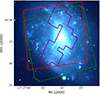 |
Fig. 1. Optical image of NGC 4242 using the grz filters from the Legacy Survey DR6 (Dey et al. 2019) and the GULP (F150LP in purple, and F218W in green) and LEGUS mosaics (F275W in red). |
While the UV filters can be used to detect young massive stars, star clusters, and OB associations, the wide photometric coverage helps us to better constrain the spectral energy distributions (SEDs) between ∼1500 Å and ∼8100 Å of these high-mass stars. This results in better estimates of their age and mass. Furthermore, the UV filters are key factors to quantify how strongly and efficiently ultraviolet light emitted by massive stars is absorbed by dust grains.
The observing dates, instruments, filters, and exposure times are reported in Table 1. All the frames were aligned to Gaia Data Release 3 (Gaia Collaboration 2021) and drizzled to a common pixel scale of 0.04″/px (the native WFC3 pixel size) using the F438W frame as reference.
Observation log.
Fluxes for point-like sources in the F275W, F336W, F438W (reference frame), F555W, and F814W filters were measured via PSF-fitting using the WFC3 module of the photometry package DOLPHOT version 2.0 (Dolphin 2000, 2016). The list of stars detected by DOLPHOT in the F275W filter was then used as input to perform aperture photometry in the filters F150LP and F218W using the Astropy package Photutils (Sabbi et al., in prep.). The aperture radius around each object was 3 pixel, and an annulus with an inner radius 12 pixels and a width of 2 pixels was used for the sky subtraction. All the magnitudes are in the Vegamag system.
2.1. The stellar photometric catalog
To correctly study the properties of massive stars, we needed to remove as many extended objects or spurious detections as possible. We did this in two steps. First, we applied selection criteria on the photometric error, sharpness, and roundness of objects observed in the F438W and F555W filters. All sources with a photometric error larger than 0.3 mag and |roundness| > 2 were removed. A further constraint was placed on the sharpness: objects whose sharpness deviated by more than 1σ from the 50th percentile value per magnitude bin were discarded. Figure 2 shows the change in the photometry quality as a function of the magnitude in the B filter. The black points represent the full catalog, and the red points show the sources that passed the full selection process.
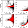 |
Fig. 2. Quality of the PSF photometry for the sources detected by LEGUS in the F438W (B) filter. In each panel, the black dots refer to the full sample, and the red points indicate sources that passed the full selection process, as described in Sect. 2.1. |
As a second step, we only considered the sources with a flux detection in the F275W filter out of the sources that passed the criteria above. Stars that were observed in one or both of the FUV and MUV filters were only selected when their photometric errors in these filters were smaller than 0.3 mag. At the end of the selection phase, we had sources that were only observed in the LEGUS filters (from the NUV to the I band), stars that were observed in all the filters (from the FUV to the I band), and sources with only one GULP flux. In fact, for this galaxy, GULP and LEGUS observations do not completely overlap, and we did not want to miss any massive star candidates (see Fig. 1).
2.2. Star cluster and OB association catalog
The LEGUS collaboration identified candidate star clusters and OB associations in the star-forming galaxies observed by the survey (Adamo et al. 2017; Grasha et al. 2017). We summarize their procedure here.
An automatic pipeline extracted candidates and computed the concentration index (CI). The concentration index is defined as the magnitude difference between apertures at radii of 1 pixel and 3 pixels. A sample of isolated and bright stars was used to set the threshold CI value between stars and candidate star clusters. For NGC 4242, the threshold value was 1.3 mag for the WFC3 F555W filter. The CI cut allows the user to remove a large number of stars from the catalog. However, compact and unresolved candidate star clusters whose effective radius is 1 pc or smaller might be removed by the CI cut. Multi-band aperture photometry and averaged aperture corrections were performed for each target whose CI was higher than the threshold value. In order to remove possible outliers, the sources from the automatic catalog were visually inspected. All the candidates that were observed in at least four bands with a photometric error smaller than 0.3 mag and whose F555W absolute magnitude was brighter than −6 mag were visually inspected. During the visual inspection, sources that were clearly clusters and were missed during the automatic procedure were added to the catalog. The visually inspected sources were then divided into four classes. Class 1 objects are centrally concentrated objects whose full width at half maximum (FWHM) is more extended than that of a star. Class 2 objects have a less symmetric light distribution, and Class 3 objects are characterized by a multi-peak light distribution. Finally, Class 4 objects are potentially single stars or artifacts.
The physical properties of the candidates (e.g., age, mass, and dust extinction) were obtained using the SED fitting techniques described by Adamo et al. (2017). We used the catalog based on Yggdrasil SSP models (Zackrisson et al. 2011) with a Kroupa initial mass function (IMF; Kroupa 2001), nebular continuum and emission lines with a covering factor 0.5, a metallicity Z = 0.02, Padova isochrones (Marigo et al. 2008; Girardi et al. 2010; Tang et al. 2014; Chen et al. 2015), and a MW extinction law (Cardelli et al. 1989). Figure 3 shows the mass and age distribution of Class 1 + Class 2, and Class 3 objects. In particular, it shows that a large fraction of clusters at young ages (≤15 Myr) have a low mass. This trend is used in Sect. 4 to refine the cluster sample.
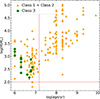 |
Fig. 3. Mass and age distribution of clusters or OB associations identified by the LEGUS collaboration using the theoretical models described in Sect. 2.2. The red lines correspond to the 100 M⊙ cutoff and the 15 Myr cutoff used in Sect. 4. |
2.3. Hα and infrared images
In order to explore the environment around our massive star candidates, we used auxiliary Hα and infrared images. In particular, we used the stellar continuum-subtracted Hα image taken by Kennicutt et al. (2008) with the Bok Telescope to identify the ionized regions around massive stars.
For the dust distribution in NGC 4242, we used the infrared maps obtained by Dale et al. (2009) using the Spitzer Telescope. The Infrared Array Camera (IRAC) 8.0 μm image provides information on the polycyclic aromatic hydrocarbon (PAH) molecules, while the Multiband Imaging Photometer (MIPS) 24.0 μm maps show the hot dust. We removed the stellar emission to obtain the pure PAH and hot-dust emission using the 3.6 μm as continuum. We computed the stellar PSF of the 3.6, 8.0 and 24.0 μm images. The pixel scale for the 3.6 and 8.0 μm data is 0.75″/px, and it is 1.5″/px for the 24.0 μm data. We convolved the 3.6 μm image with the 8.0 μm PSF and the 8 μm image with the 3.6 μm PSF using the IRAF function convolve. In order to account for the different pixel scale of the 24.0 μm image, we first magnified the 3.6 μm image and the PSF using the magnify function in IRAF, and we then convolved it with the 24 μm image and the PSF. The convolved images were then subtracted using the equation presented by Helou et al. (2004) and Dale et al. (2009),
 (1)
(1)
and we repeated this for the 24.0 μm image, where ν is the frequency, fν is the specific flux density, η8* = 0.232 × 3.6/8.0 for the 8.0 μm image, and η24* = 0.032 × 3.6/24.0 for the 24.0 μm map. We refer to these stellar continuum-subtracted images as “pure” Hα, 8.0 μm, and 24.0 μm images.
3. Identification and characterization of massive stars
Color-magnitude diagrams (CMDs) are useful tools for interpreting the resolved stellar component in the host galaxy. The emission of massive stars peaks at ultraviolet wavelengths, which makes them bright objects in the UV filters of the GULP and LEGUS surveys. The dust component of the host galaxy absorbs a large fraction of the ultraviolet light, however, and re-emits it at longer wavelengths. Moreover, different empirical extinction laws for different environments have been found. It is therefore crucial to determine the correct extinction law for NGC 4242 in order to interpret the properties of its massive stars.
3.1. Extinction law
The change in extinction as a function of the wavelength was measured for a number of galaxies, including the MW (Cardelli et al. 1989; Fitzpatrick 1999) and the Magellanic Clouds (Nandy & Morgan 1978; Gordon et al. 2003; Maíz Apellániz & Rubio 2012). While the MW extinction law exhibits a bump in the absorption of photons at a wavelength of 2175 Å (the so-called UV-bump), the SMC extinction law does not.
We first removed the Galactic foreground extinction using Cardelli et al.’s (1989) extinction law and a value of AV = 0.033 mag (Schlafly & Finkbeiner 2011). We then used the mixture model from Gordon et al. (2016) with MW and SMC components to determine the effect of extinction on the photometry of our data. This model depends on the total-to-selective extinction ratio, RV, and fA which regulates the amount of extinction from the MW component alone (see Gordon et al. 2016). We chose the RV and fA parameters by visually inspecting the V-I and UV Hess diagrams in two steps. First, we varied the RV value to match the V-I Hess diagram. Then, keeping RV fixed, we fine-tuned the fA parameter with the aim to match the blue edge in the FUV-B and MUV-B Hess diagrams. We found that the distribution of stars in different Hess diagrams (from the FUV to the I band) is well described by Padova isochrones (Marigo et al. 2008; Girardi et al. 2010; Tang et al. 2014; Chen et al. 2015) using a true distance modulus μ = 28.61 mag, an intrinsic extinction of E(B − V) = 0.05 mag, and a metallicity Z = 0.02 (Sabbi et al. 2018) for the pair (RV, fA) = (3.1, 1.0). This corresponds to the MW extinction law (Fitzpatrick 1999 with RV = 3.1) for NGC 4242. Figure 4 shows the Hess diagrams, and the Padova isochrones corrected for extinction using RV = 3.1 and fA = 1.0 are overplotted.
 |
Fig. 4. Hess diagrams for different combinations of filters. The Padova isochrones for different ages are overplotted using Z = 0.02, E(B − V) = 0.05 mag, a distance modulus μ = 28.61 mag (Sabbi et al. 2018), and the extinction coefficients from the Gordon et al. (2016) model with RV = 3.1 and fA = 1.0. The black arrow indicates the reddening vector using AV = 0.5 mag. |
3.2. Age separation
We decided to differentiate stars according to their age estimated via the F150LP versus F150LP–F814W, F814W versus F150LP–F814W, F218W versus F218W–F814W, and F275W versus F275W–F814W CMDs. Figure 5 shows the four different CMDs using Padova isochrones and the extinction parameters from Sect. 3.1. The stars were divided in age ranges according to their position within two consecutive isochrones.
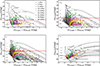 |
Fig. 5. Color-magnitude diagrams used to differentiate stars according to age. The Padova isochrones for ages 1, 3, 5, 10, 15, 20, 25, 30, 40, and 50 Myr, a metallicity Z = 0.02, a distance modulus μ = 28.61 mag, and intrinsic E(B − V) = 0.05 mag are superimposed. The extinction coefficients were taken from the model of Gordon et al. (2016) with RV = 3.1 and fA = 1.0. The stars are color-coded by the age determined based on their positions between consecutive isochrones in each CMD. The black points show stars that do not lie in between consecutive isochrones. The dashed red line shows the luminosity of a main-sequence star with Mini = 15 M⊙ and an age of 10 Myr. The black arrow indicates the reddening vector using AV = 0.1 mag. |
We were only interested in massive and young objects, and we therefore removed all the objects with an initial mass lower than 15 M⊙ from each CMD. Using Padova isochrones and a foreground MW extinction AV = 0.033 mag (Schlafly & Finkbeiner 2011), we removed all the objects fainter than 24.7, 21.4, 22.2, and 21.8 mag for the F814W, F150LP, F275W, and F218W filters, respectively. Schneider et al. (2018) analyzed 173 O stars in 30 Doradus finding an average maximum age of about 10 Myr. We therefore decided to consider objects in the age range 1 − 10 Myr. Stars that are bluer than the 1 Myr isochrone (possibly due to photometric errors, uncertainty on the metallicity, the extinction law, and theoretical models) were also taken into account. At this point, stars younger than 10 Myr and brighter than the magnitude cut in at least one of these CMDs were considered. We selected 242 objects from the four CMDs. Assuming that these objects are single non-rotating stars, we estimated their initial mass (Mini), age, and intrinsic extinction (AV) based on their photometry by minimizing the difference between the observed and theoretical magnitudes. Let yobs and σ be the vectors of the observed magnitudes and photometric errors, and yth the vector of the synthetic reddened magnitudes derived from the Padova isochrones. In the theoretical models, the age varies between 1 and 10 Myr with steps of 0.2 Myr, Mini varies between 0.08 and 350 M⊙, and AV ranges from 0.0 to 1.0 mag with steps of 0.01 mag. We computed the χ2 for the single model as
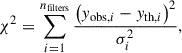 (2)
(2)
and the sum was run over the number of filters. The minimum χ2 gave the best (log t, Mini, and AV) triplet. To estimate the error on each parameter, we perturbed the observed photometry of each star using a multivariate normal distribution, 𝒩(μ = yobs, σ2 = σ2), centered on the observed photometry and with the photometric errors as its σ. We ran 100 Monte Carlo iterations for each star and took the standard deviations of the 100 best triplets as the corresponding errors of each parameter.
The χ2 confirmed that 234 sources are younger than 10 Myr and have an initial mass higher than 15 M⊙. The fluxes of 100 stars are available in all filters, for 110 stars only one GULP flux is available, and the remaining stars (24) only have LEGUS fluxes (see Sect. 2.1 and Fig. 1).
Figure 6 shows the best values obtained for AV, age, and Mini, color-coded by the degree of freedom (d.o.f. = 4 for a complete wavelength coverage, d.o.f. = 3 for only one GULP flux, and d.o.f. = 2 for a detection only in between the NUV and the I bands). The histograms show that the age and AV of our selected stars are distributed throughout the age range and the 0.0 to 1.0 mag interval, with a mean age of 5.7 Myr and an average intrinsic extinction of AV = 0.18 mag, in agreement with Sabbi et al. (2018). The majority of our stars have Mini between 15 and 100 M⊙, while some others exceed Mini = 150 M⊙ and AV = 0.4 mag. A possible explanation for the latter is the presence of a star cluster around our targets or other unresolved stars that can contaminate the photometry. Some of our targets are close to star clusters identified by LEGUS (see Adamo et al. 2017), which increases the χ2, and the parameter estimate is less precise.
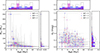 |
Fig. 6. Best values for age, AV, and Mini and their histogram distributions using Padova isochrones with a fixed metallicity Z = 0.02, an age range of 1 − 10 Myr, and a varying intrinsic extinction AV ∈ [0.0, 1.0] based on the extinction coefficients from Gordon et al. (2016) for RV = 3.1 and fA = 1.0 (Sect. 3.1). The targets are divided in three groups based on the degrees of freedom, which depend on the number of available filters as explained in Sect. 2.1 (d.o.f. = 4 for a complete wavelength coverage, d.o.f. = 3 for one GULP flux alone, and d.o.f. = 2 for detection only in between the NUV and the I bands). The histograms are normalized to the total number of sources. The dashed black histogram shows the total frequency. |
In order to test how our derived stellar ages, initial masses, and dust extinctions depend on the metallicity of the isochrone and on the extinction law assumed for NGC 4242, we fit the observed photometry using three different setups: Padova isochrones with an SMC metallicity reddened with a MW extinction law, Padova isochrones with solar metallicity and an SMC extinction law (RV = 2.74 Gordon et al. 2003), and Padova isochrones with an SMC metallicity and an SMC extinction law. We found that at fixed metallicity, the average age of our sample becomes younger by 1 Myr and the average extinction slightly increases by 0.01 mag, while at fixed extinction law, the population becomes older by 1 Myr and the extinction increases by no more than 0.02 mag. The results are described in Appendix A.
3.3. Spatial distribution of the targets
We expect to find massive and young objects along the spiral arms of NGC 4242. Figure 7 shows the spatial distribution of the targets grouped into four different age bins. We used the stellar continuum-subtracted Hα image taken by Kennicutt et al. (2008) with the Bok Telescope to connect young targets with Hα emission (drawn in magenta). The comparison between Figs. 1 and 7 shows that most of the targets are distributed along the faint spiral arms of NGC 4242, as delineated by the Hα emission in Fig. 7.
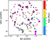 |
Fig. 7. Spatial distribution of the selected targets grouped into four different age bins. The underlying pure Hα emission (in magenta) was taken by Kennicutt et al. (2008) with the Bok Telescope. |
In most of the cases, our targets are located in Hα emission regions. The left panel of Fig. 8 shows the spatial distribution of the targets color-coded by the best values for their reddening. We note that some targets need a very low reddening even when they coincide with Hα emission. We suggest that these targets are not in the Hα emission region, but in the foreground, and that the Hα is in the background within the galaxy NGC 4242. On the other hand, some targets with a high reddening are not associated with Hα emission. Stars with a high reddening value might lie behind dust lanes. The right panel of Fig. 8 shows a composite image of the pure Hα emission (in magenta), the pure 8.0 μm (in green), and the pure 24.0 μm (in orange). The dust images were taken by the Spitzer Space Telescope (Dale et al. 2009), and the stellar continuum subtraction is described in Sect. 2.3.
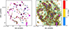 |
Fig. 8. Spatial distribution of the targets color-coded by the best value of their intrinsic extinction AV. The left panel shows the pure Hα emission in magenta. The right panel shows the underlying pure Hα in magenta, the pure 8.0 μm in green (PAH emission), and the pure 24.0 μm in orange (hot-dust emission). |
4. Isolation analysis
4.1. Isolation with respect to star clusters or OB associations
Even though massive stars are short-lived, those in the field are frequently considered to be runaways or walkaways from known star clusters or OB associations (Blaauw 1961; Poveda et al. 1967; Gies 1987; Hoogerwerf et al. 2001; Dorigo Jones et al. 2020). Thus, we used the spatial distribution of our targets and the visually inspected young star clusters and OB associations (age ≤15 Myr) from Adamo et al. (2017, see our Sect. 2.2) to determine the number of stars from our sample that might be runaways from these stellar groups. We note here that while in the MW and the SMC, the runaway or walkaway nature of a star can be tested via spectroscopic radial velocities and astrometric tangential velocities, this is not feasible with the existing instrumentation in a galaxy at the distance of NGC 4242.
The clusters can be divided into three classes according to their PSF shape: spherically symmetric, asymmetric, or multi-peak PSF (see Sect. 2.2). We grouped symmetric and asymmetric objects together, and we refer to these objects as star clusters, while multi-peak PSF objects were considered OB associations because of their larger size. We decided to only consider objects more massive than 100 M⊙ and younger than 15 Myr, which amount to 74 star clusters and only 14 OB associations, with a median separation of ∼180 pc. This is justified by the work of Hunt & Reffert (2023), who, using Gaia data, were able to identify Galactic open clusters as massive as ∼100 M⊙ that contain a few massive stars as massive as 50 M⊙.
Runaway OB stars can be produced via two main mechanisms: the dynamical ejection scenario, and the binary supernova scenario. In the former, gravitational interactions in dense clusters could eject a massive star (Blaauw 1961; Poveda et al. 1967), while in the latter, the supernova explosion could eject the companion star (Renzo et al. 2019; Blaauw 1961). Recently, Polak et al. (2024) have analyzed the production of runaways through the subcluster ejection mechanism, where stars in a subcluster can be ejected during the tidal disruption of the parent subcluster that falls into the deeper gravitational potential of the protocluster. Runaway stars are traditionally defined to have a 3D peculiar motion of at least 30 km s−1 (Gies 1987; Hoogerwerf et al. 2001), which corresponds to a transverse 2D minimum velocity of 24 km s−1 assuming equal velocity components in space (Dorigo Jones et al. 2020). Fast runaways with a velocity of 200 km s−1 in the SMC have been found by Dorigo Jones et al. (2020), but theoretical studies (Perets & Šubr 2012) showed that the runaway frequency is strongly reduced with increasing peculiar velocity. This agrees with Dorigo Jones et al. (2020), who found that the local velocity of only 48 stars out of 199 runaway stars in the SMC is higher than 75 km s−1. The authors showed that the peak of the distribution of runaway stars is reached between 30 and 75 km s−1 with a steep drop for higher velocities. A steep decrease in the distribution of runaway stars was also found for the massive star cluster R136 in the Large Magellanic Cloud (Stoop et al. 2024). Only 8 (out of 23) O-type stars are runaways from R136 with tangential velocities higher than 50 km s−1. Based on these velocities as references, a runaway star can travel tens to hundreds of parsecs in a few million years. For example, Stoop et al. (2024) found that the population of O runaway stars had traveled a mean distance of 59 pc from the center of R136, and this value reached a value of 115 pc when they also considered the runaways without a spectral classification. The theoretical studies of the BSS by Renzo et al. (2019) revealed that a main-sequence massive companion star travels ∼75 pc on average, which agrees with the 50 pc found by Eldridge et al. (2011). However, both distributions of the maximum distance are characterized by a large scatter.
We identified the closest star cluster or OB association from each star target to determine the probability that the target belongs to that stellar group. We de-projected the positions of stars, star clusters and OB associations on the galaxy plane by adopting an inclination of i = 40.5° (Calzetti et al. 2015), and then computed their 2D projected distance.
In order to take the velocity distribution found by Dorigo Jones et al. (2020) into account, we decided to take two threshold distances: dthresh, 1 = 74 pc and dthresh, 2 = 204 pc. The former corresponds to the distance traveled by a star in 1 Myr with three times the minimum 2D runaway velocity, while the latter is the distance that a fast runaway can travel in 1 Myr at 200 km s−1. These two threshold distances allowed us not only to identify runaway candidates with the former velocities and 1 Myr travel time, but also runaways with a combination of velocities and travel times. For example, the dthresh, 2 can help us identify runaway stars with the minimum 2D runaway velocity that have traveled for ∼8 Myr.
Number and frequency of possible isolated stars relative to nearby clusters or OB associations.
Every star that has a star cluster (or OB association) closer than the threshold distance was considered a possible walkaway or runaway from that particular group, otherwise, it was considered to be in isolation (method 1). Each circle in Fig. 9 shows the location of the closest star cluster or OB association for each star with d.o.f. = 4. When a star is found near to a star cluster, this does not imply that they are connected. We decided to also use the age information, and selected stellar groups whose age differed by 5 Myr at most from the age of the star. We then searched for the closest cluster or OB association (method 2). The range of 5 Myr takes the age spread of O-type stars found in Cygnus OB2 (Berlanas et al. 2020) and in the massive star cluster R136 (Schneider et al. 2018) into account. Moreover, it corresponds to the maximum error on the age of our stars as computed in Sect. 3.2. The mean error on the age of a star from the isochrone fitting is 1.8 Myr, while the maximum error is 5 Myr. We chose the latter as the maximum age difference between a star and a cluster to create possible connections between them. Each square in Fig. 9 shows where the closest star cluster (or OB association) is located for each star with a similar age. The stars are divided into age bins. The two methods for the distances found the same connection between star and stellar groups in some cases (no connecting dashed line), while some stars appeared to be close to a stellar group whose age difference is more than 5 Myr. This means that their connections are less likely true, and increases the probability that they are unrelated to those stellar groups.
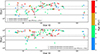 |
Fig. 9. De-projected distances between stars with d.o.f. = 4 and star clusters (top panel) or OB associations (bottom panel). On the x-axis, we show the star ID from the sample. The circles show the distance of the closest cluster from each target (method 1), and the squares show the closest cluster with an age similar to that of each star (method 2). The dashed vertical black lines connect the distances from method 1 and method 2 when they find two different stellar groups. The symbols are color-coded according to the derived age of the stars. The horizontal gray lines show the maximum tangential distances that a star can travel in 1 Myr with a constant velocity of 24 km s−1, 100 km s−1, and 200 km s−1. These distances are 24, 102, and 204 pc (horizontal solid, dot-dashed, and dotted lines, respectively). At a distance of 5.3 Mpc, 1 pc is 0.039 arcsec. |
Following the age bins in Fig. 9, we computed the median separation between stars and their nearest cluster (or OB association) using methods 1 and 2. For the star clusters, we found a positive correlation. The median distance between young stars and star clusters increased toward older age bins, but this trend became weaker for method 2. On the other hand, for younger age bins, OB associations were found to be closer to young stars, and the trend disappeared using method 2. The different trend between clusters and OB associations is most likely due to the small number statistics of the latter.
Fig. 10 shows the connections between star and star clusters (or OB associations) we were able to find as a function of the projected distance. The figure shows that there are stars located far away from known star clusters or OB associations, being potentially isolated. Table 2 summarizes the number of isolated objects given the method or the threshold value. Some of our stars might have traveled a longer distance (with a higher runaway velocity or for a longer time) and might contaminate the isolated star sample. Conversely, stars in projected proximity to clusters or OB associations might be unrelated to them.
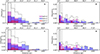 |
Fig. 10. Distance distributions. Panels A and B show the simple projected 2D distance between our stars and the nearest star cluster and OB association, respectively. Panels C and D show the distances from the nearest star cluster or OB association that differ by 5 Myr at most from the estimated stellar ages. The sample is color-coded according to the degree of freedom, and each histogram is normalized to the total number of stars in the sample. The dashed black histogram shows the total frequency. All bins have an equal size of 100 pc. The vertical black lines show the distances that a star can travel in 1 Myr with a constant velocity of 24 km s−1, 100 km s−1, and 200 km s−1. These distances are 24, 102, and 204 pc. |
4.2. Isolation with respect to other massive stars
Another criterion for the isolation is that no other massive and young object is found in the vicinity of each target. Following Dorigo Jones et al. (2020) and Renzo et al. (2019), we also investigated the isolation of each target with respect to other massive and young stars from our sample. We decided to consider method 1 and the two threshold distances as constraints for the isolation from other massive stars. Table 3 shows the number of objects without known young stellar groups and other massive and young stars nearby for different threshold distances. The new constraint implies a reduction in the isolation frequencies. Regardless of the method and the threshold value used, the final frequency of potentially isolated objects is never zero.
Number and frequency of possible isolated stars relative to nearby clusters, OB associations and massive stars.
This final sample contains two types of objects: stars that might have been formed in situ in the field in isolation (or with a small population of low-mass stars around them), and possible runaways that traveled for a longer period of time than the travel times we considered, or they traveled with higher velocities.
5. Discussion
We investigated the environment around 234 young massive star candidates in order to study the phenomenon of possible isolated massive star formation. In the previous section, we examined the possibility that some of our targets might be runaways from known star clusters or OB associations. Regardless of whether runaway objects are produced via binary supernova, dynamical ejection, or subcluster ejection mechanisms, their peculiar velocity in the galaxy plane is 24 km s−1 at least (Dorigo Jones et al. 2020). Considering this velocity as the typical velocity of runaways, we set dthresh, 1 = 74 pc as the first threshold distance typically traveled by a runaway. We found with method 1 that 68%±6% ( = 159/234) of the stars in the sample lie at a larger distance and have no known young star clusters and OB associations around them.
There is evidence that some stars can reach very high runaway velocities (Dorigo Jones et al. 2020; Sana et al. 2022). In order to remove possible fast runaways from our sample, we adopted dthresh, 2 = 204 pc as our second threshold distance. As a consequence, the fraction of possible isolated stars with respect to star clusters and OB associations using method 1 decreased to 34%±4% ( = 79/234).
We set the minimum threshold (dthresh, 1) to three times the distance traveled by a runaway star in 1 Myr at the minimum 2D velocity. This not only enabled the selection of stars that might move at higher velocities or for longer times, but also accounted for the uncertainty of ∼0.5 Mpc in the distance of NGC 4242 (Sabbi et al. 2018). For very high velocities, the number of very fast runaways drops sharply with the velocity (Perets & Šubr 2012; Dorigo Jones et al. 2020). Increasing dthresh, 2 would lead to a large number of connections between stars and clusters, not all of which are necessarily true. We expect to miss only a few faster runaways because there are so few of them. Moreover, these two threshold distances allowed us not only to identify runaway candidates traveling for only 1 Myr at the two constant velocities, but also runaways with a combination of velocities and travel times.
The possible connections between stars and stellar groups were only based on the projected distance. When the similarity in age between stars and stellar groups is also considered, the number of possible physical connections decreases. We assumed a maximum age difference between a star and a star cluster (or OB association) of 5 Myr. This age difference reflects the age spread that Berlanas et al. (2020) and Schneider et al. (2018) found for massive stars in Cygnus OB2 and R136, respectively. Moreover, 5 Myr corresponds to the maximum age error we obtained for our sample, and it is consistent with the age discrepancy of 0.2 dex found by Stevance et al. (2020) between single-star isochrone and binary SED fitting with BPASS (Binary Population and Spectral Synthesis). This uncertainty only affects method 2, but the results from method 1 are not affected.
Ten (for dthresh, 1) or twenty-four (for dthresh, 2) stars that we previously associated with star clusters or OB associations as possible runaways differ by more than 5 Myr from those stellar groups, which makes these links less likely to be physical. The resulting fractions of possible isolated objects using method 2 become 72%±6% ( = 169/234) and 44%±4% ( = 103/234) for dthresh, 1 and dthresh, 2, respectively.
A further constraint was the isolation with respect to other massive stars outside of clusters. Depending on the threshold distance and method, the frequency varied from a minimum of 9.8%±2% (= 23/234 for dthresh, 2 and method 1) to a maximum of 34.6%±3% (= 81/234 for dthresh, 1 and method 2). The errors are for Poisson statistics alone.
Observations suggest that 4%±2% of all O stars in the MW appear to be isolated from known star clusters and OB associations and cannot be interpreted as runaways (de Wit et al. 2005). This result is consistent with Vargas-Salazar et al. (2020), who found that 4 − 5% of O type stars in the field of the SMC appear to be isolated from star clusters and OB associations, but these authors also observed small clustering of low-mass stars around these seemingly isolated massive stars. Parker & Goodwin (2007) found that the fraction of sparse star clusters (M < 100 M⊙) with only one massive O-type star varied between 1.3% and 4.6% for a cluster mass function exponent of β = 1.7 and β = 2, respectively.
In order to compare our findings with those of de Wit et al. (2005), we computed the expected number of massive stars (Mini ≥ 15 M⊙) that did not explode as a supernova at 10 Myr. We computed the SFR(UV) directly from the GALEX FUV image (Lee et al. 2009) in the F275W HST footprint, using the equation presented by Kennicutt (1998), a distance of 5.3 Mpc, and the correction for the Galactic foreground extinction from Schlafly & Finkbeiner (2011). This resulted in a SFR(UV) = 0.038 M⊙ yr−1. We corrected this star formation rate for the intrinsic mean extinction found in Sect. 3.2, obtaining SFR(UV) = 0.057 M⊙ yr−1. We also estimated the SFR(Hα) from the Bok image in the F275W HST footprint, following the flux calibration described by Kennicutt et al. (2008) and using the equation presented by Kennicutt (1998). We applied the same distance and foreground and intrinsic extinction corrections (using the mean extinction from Sect. 3.2 using solar metallicity and a MW-like extinction law) and used the star-to-gas extinction conversion from Calzetti et al. (2000). We found that the SFR(Hα) is 57% lower than the SFR(UV), which agrees with the value found by Lee et al. (2009). Different studies of H II regions in galaxies with different metallicities, masses, and SFRs have shown that the escape fraction of the ionizing photons can reach values of about 67% (Della Bruna et al. 2021; Ramambason et al. 2022; Egorov et al. 2018; Gerasimov et al. 2022; Pellegrini et al. 2012). The large escape fraction can lead to an underestimation of the SFR(Hα) of up to a factor of three. Therefore, we decided to assume a constant SFR = 0.057 M⊙ yr−1 from the GALEX FUV over the last 100 Myr to compute the expected number of massive stars in our HST footprint. We computed the expected number of massive stars that did not yet explode as a supernova using the equation presented by Kim et al. (2013),
 (3)
(3)
where Ṁ∗ = 0.057 M⊙ yr−1 is the dust-corrected SFR(UV), Δt = 10 Myr is our age range, and m* = 812 M⊙ is the total mass in massive stars that have not yet exploded as a supernova. The latter was computed using a Kroupa IMF (Kroupa 2001) and a mass range 15 − 18.88 M⊙. These two masses are the lower initial mass for our sample and the upper limit for a star that survives for 10 Myr without exploding. We found that the expected number of massive stars in the field and stellar groups for our mass and age limits is ∼707 objects. For the expected total number of massive stars, the fraction of possible isolated objects is 3.2 ± 0.7%−11.5 ± 1.3%. The value 11.5% we found for a threshold of 74 pc is higher by a factor of three than what was reported by de Wit et al. (2005), who used a threshold of 65 pc.
We recomputed the fraction of candidate isolated massive stars using the stellar parameters obtained in Appendix A for the three different setups described in Sect. 3.2. For solar metallicity and SMC-like extinction, the fractions vary between 2.2 ± 0.5%−7.6 ± 0.9% because the average extinction is higher, and consequently, the dust-corrected SFR(UV) is higher, while the fractions become higher for an SMC-like metallicity with a MW-like extinction law (3.3 ± 0.6%−12.0 ± 1.2%). Finally, the combination of an SMC metallicity with the SMC-like extinction law gives fractions in between 2.1 ± 0.4%−7.6 ± 0.7% (see Appendix A).
We note that our fractions of isolated massive star candidates are upper limits. The cluster catalog only contains cluster candidates that were visually inspected and whose effective radius is at least 1 parsec (see Adamo et al. 2017). Potentially unresolved clusters with sizes of 1 parsec and smaller might be missed. These compact star clusters can reduce the number of possible isolated objects. On the other hand, this is mitigated by the requirement that other massive stars around each target were avoided. Moreover, the distinction between possible runaways from star clusters and isolated objects was only based on position information and not on local velocities for our targets. The runaway nature of a star can be tested via spectroscopic radial velocities and astrometric tangential velocities in the MW and SMC, but this is not feasible in a galaxy at the distance of NGC 4242. Therefore, some of our final targets might still be very fast runaways or might have traveled longer from their original birthplace. Finally, some of the isolated candidates might be surrounded by an undetected clustering of low-mass stars (Vargas-Salazar et al. 2020) that we are not able to detect. Conversely, we might be missing truly isolated stars that are seen to lie close to clusters or OB associations in projection.
6. Conclusions
In summary, we carried out a galaxy-wide search of massive stars throughout the entire galaxy NGC 4242 using far- and mid-ultraviolet data from HST to find young massive stars that are isolated with respect to star clusters, OB associations, and other massive stars. We first presented the identification of possible single young massive field stars by exploiting the F150LP and F218W fluxes from ACS/SBC and WFC3 from HST and identified 234 candidates. We then analyzed the surroundings of these targets and searched for young (≤15 Myr) star clusters and OB associations identified in the LEGUS survey (Adamo et al. 2017). In fact, massive stars can be ejected from star clusters or OB associations and become runaways or walkaways.
We set two threshold distances, 74 and 204 pc. The former corresponds to three times the distance traveled by a massive star in 1 Myr with the minimum 2D velocity of 24 km s−1, while the latter corresponds to the distance traveled by a fast runaway in the same time interval with a velocity of 200 km s−1. Every star closer to a star cluster or OB association than the threshold distance might be a potential runaway from that star group. We decided to analyze the isolation of our targets based not only on their positions, but also on the similarity in age between stars and star clusters or OB associations. In this second method, we investigated the spatial distribution of star clusters and OB associations with differences in age smaller than 5 Myr from the estimated age of the selected massive star.
The surroundings of the possible isolated objects were then analyzed, and other massive stars were searched for. Depending on the method and threshold distance, the frequency for isolation in the field of NGC 4242 varies from 9.8% to 34.6%, using dthresh, 2 and dthresh, 1, respectively. These fractions reduce to 3.2 ± 0.7%−11.5 ± 1.3% when they are computed with respect to the total expected population of massive stars in the galaxy, with the latter larger by a factor of three than what was reported by de Wit et al. (2005) for the MW. However, our fractions are upper limits to the fraction of truly isolated massive stars. We cannot probe the possible clustering of low-mass stars around our targets, that is, we cannot exclude the presence of very sparse star clusters. The fraction of apparently isolated massive stars around which faint clustering of low-mass stars was found is 4 − 5% in the SMC (Vargas-Salazar et al. 2020). Moreover, our results can still be affected by very fast runaways or objects that have traveled for a longer period of time. Conversely, we might be missing truly isolated stars located in close apparent proximity to star clusters due to projection effects.
This is the first study that searched for isolated massive stars in a galaxy beyond the immediate neighborhood of the Milky Way. Overall, we found a fraction of potentially isolated massive stars similar to the early work for the MW and Magellanic Clouds (de Wit et al. 2005). Future studies at higher resolution are needed to elucidate this issue further.
Acknowledgments
We thank the anonymous referee for the constructive comments that helped improving the paper. The HST observations used in this paper are associated with program No. 16316 and No. 13364. This work is based on observations obtained with the NASA/ESA Hubble Space Telescope, at the Space Telescope Science Institute, which is operated by the Association of Universities for Research in Astronomy, Inc., under NASA contract NAS 5-26555. E.S. is supported by the international Gemini Observatory, a program of NSF NOIRLab, which is managed by the Association of Universities for Research in Astronomy (AURA) under a cooperative agreement with the U.S. National Science Foundation, on behalf of the Gemini partnership of Argentina, Brazil, Canada, Chile, the Republic of Korea, and the United States of America. J.S.G. acknowledges grant support under these GO programs from the Space Telescope Science Institute which is operated by the Association of Universities for Research in Astronomy, Inc., under NASA contract NAS 5-26555. A.A. acknowledges support from Vetenskapsrådet 2021-05559. RSK acknowledges financial support from the ERC via Synergy Grant “ECOGAL” (project ID 855130), from the German Excellence Strategy via the Heidelberg Cluster “STRUCTURES” (EXC 2181 – 390900948), and from the German Ministry for Economic Affairs and Climate Action in project “MAINN” (funding ID 50OO2206). RSK also thanks the 2024/25 Class of Radcliffe Fellows for highly interesting and stimulating discussions. The Legacy Surveys consist of three individual and complementary projects: the Dark Energy Camera Legacy Survey (DECaLS; Proposal ID #2014B-0404; PIs: David Schlegel and Arjun Dey), the Beijing-Arizona Sky Survey (BASS; NOAO Prop. ID #2015A-0801; PIs: Zhou Xu and Xiaohui Fan), and the Mayall z-band Legacy Survey (MzLS; Prop. ID #2016A-0453; PI: Arjun Dey). DECaLS, BASS and MzLS together include data obtained, respectively, at the Blanco telescope, Cerro Tololo Inter-American Observatory, NSF’s NOIRLab; the Bok telescope, Steward Observatory, University of Arizona; and the Mayall telescope, Kitt Peak National Observatory, NOIRLab. Pipeline processing and analyses of the data were supported by NOIRLab and the Lawrence Berkeley National Laboratory (LBNL). The Legacy Surveys project is honored to be permitted to conduct astronomical research on Iolkam Du’ag (Kitt Peak), a mountain with particular significance to the Tohono O’odham Nation.
References
- Adamo, A., Ryon, J. E., Messa, M., et al. 2017, ApJ, 841, 131 [Google Scholar]
- Berlanas, S. R., Herrero, A., Comerón, F., et al. 2020, A&A, 642, A168 [NASA ADS] [CrossRef] [EDP Sciences] [Google Scholar]
- Blaauw, A. 1961, Bull. Astron. Inst. Netherlands, 15, 265 [NASA ADS] [Google Scholar]
- Bonnell, I. A., Vine, S. G., & Bate, M. R. 2004, MNRAS, 349, 735 [Google Scholar]
- Calzetti, D., Armus, L., Bohlin, R. C., et al. 2000, ApJ, 533, 682 [NASA ADS] [CrossRef] [Google Scholar]
- Calzetti, D., Lee, J. C., Sabbi, E., et al. 2015, AJ, 149, 51 [Google Scholar]
- Cardelli, J. A., Clayton, G. C., & Mathis, J. S. 1989, ApJ, 345, 245 [Google Scholar]
- Chen, Y., Bressan, A., Girardi, L., et al. 2015, MNRAS, 452, 1068 [Google Scholar]
- Dale, D. A., Cohen, S. A., Johnson, L. C., et al. 2009, ApJ, 703, 517 [Google Scholar]
- de Wit, W. J., Testi, L., Palla, F., Vanzi, L., & Zinnecker, H. 2004, A&A, 425, 937 [NASA ADS] [CrossRef] [EDP Sciences] [Google Scholar]
- de Wit, W. J., Testi, L., Palla, F., & Zinnecker, H. 2005, A&A, 437, 247 [NASA ADS] [CrossRef] [EDP Sciences] [Google Scholar]
- Deharveng, L., Zavagno, A., Schuller, F., et al. 2009, A&A, 496, 177 [NASA ADS] [CrossRef] [EDP Sciences] [Google Scholar]
- Della Bruna, L., Adamo, A., Lee, J. C., et al. 2021, A&A, 650, A103 [NASA ADS] [CrossRef] [EDP Sciences] [Google Scholar]
- Dey, A., Schlegel, D. J., Lang, D., et al. 2019, AJ, 157, 168 [Google Scholar]
- Dolphin, A. 2016, Astrophysics Source Code Library [record ascl:1608.013] [Google Scholar]
- Dolphin, A. E. 2000, PASP, 112, 1383 [Google Scholar]
- Dorigo Jones, J., Oey, M. S., Paggeot, K., Castro, N., & Moe, M. 2020, ApJ, 903, 43 [NASA ADS] [CrossRef] [Google Scholar]
- Egorov, O. V., Lozinskaya, T. A., Moiseev, A. V., & Smirnov-Pinchukov, G. V. 2018, MNRAS, 478, 3386 [NASA ADS] [CrossRef] [Google Scholar]
- Eldridge, J. J., Langer, N., & Tout, C. A. 2011, MNRAS, 414, 3501 [NASA ADS] [CrossRef] [Google Scholar]
- Elmegreen, B. G., & Lada, C. J. 1977, ApJ, 214, 725 [Google Scholar]
- Fitzpatrick, E. L. 1999, PASP, 111, 63 [Google Scholar]
- Gaia Collaboration (Brown, A. G. A., et al.) 2021, A&A, 649, A1 [NASA ADS] [CrossRef] [EDP Sciences] [Google Scholar]
- Gallazzi, A., Charlot, S., Brinchmann, J., White, S. D. M., & Tremonti, C. A. 2005, MNRAS, 362, 41 [Google Scholar]
- García, B., & Mermilliod, J. C. 2001, A&A, 368, 122 [NASA ADS] [CrossRef] [EDP Sciences] [Google Scholar]
- Gerasimov, I. S., Egorov, O. V., Lozinskaya, T. A., Moiseev, A. V., & Oparin, D. V. 2022, MNRAS, 517, 4968 [NASA ADS] [CrossRef] [Google Scholar]
- Gies, D. R. 1987, ApJS, 64, 545 [NASA ADS] [CrossRef] [Google Scholar]
- Girardi, L., Williams, B. F., Gilbert, K. M., et al. 2010, ApJ, 724, 1030 [NASA ADS] [CrossRef] [Google Scholar]
- Gordon, K. D., Clayton, G. C., Misselt, K. A., Landolt, A. U., & Wolff, M. J. 2003, ApJ, 594, 279 [NASA ADS] [CrossRef] [Google Scholar]
- Gordon, K. D., Fouesneau, M., Arab, H., et al. 2016, ApJ, 826, 104 [NASA ADS] [CrossRef] [Google Scholar]
- Grasha, K., Calzetti, D., Adamo, A., et al. 2017, ApJ, 840, 113 [NASA ADS] [CrossRef] [Google Scholar]
- Helou, G., Roussel, H., Appleton, P., et al. 2004, ApJS, 154, 253 [NASA ADS] [CrossRef] [Google Scholar]
- Hoogerwerf, R., de Bruijne, J. H. J., & de Zeeuw, P. T. 2001, A&A, 365, 49 [NASA ADS] [CrossRef] [EDP Sciences] [Google Scholar]
- Hunt, E. L., & Reffert, S. 2023, A&A, 673, A114 [NASA ADS] [CrossRef] [EDP Sciences] [Google Scholar]
- Kennicutt, R. C., Lee, J. C., Funes, J. G., et al. 2008, ApJS, 178, 247 [NASA ADS] [CrossRef] [Google Scholar]
- Kennicutt, R. C. 1998, ARA&A, 36, 189 [NASA ADS] [CrossRef] [Google Scholar]
- Kim, C.-G., Ostriker, E. C., & Kim, W.-T. 2013, ApJ, 776, 1 [NASA ADS] [CrossRef] [Google Scholar]
- Kroupa, P. 2001, MNRAS, 322, 231 [NASA ADS] [CrossRef] [Google Scholar]
- Krumholz, M. R., Klein, R. I., McKee, C. F., Offner, S. S. R., & Cunningham, A. J. 2009, Science, 323, 754 [Google Scholar]
- Lada, C. J., & Lada, E. A. 2003, ARA&A, 41, 57 [Google Scholar]
- Lamb, J. B., Oey, M. S., Werk, J. K., & Ingleby, L. D. 2010, ApJ, 725, 1886 [Google Scholar]
- Lee, J. C., Gil de Paz, A., Kennicutt, R. C., et al. 2011, ApJS, 192, 6 [CrossRef] [Google Scholar]
- Lee, J. C., Gil de Paz, A., Tremonti, C., et al. 2009, ApJ, 706, 599 [NASA ADS] [CrossRef] [Google Scholar]
- Maíz Apellániz, J., & Rubio, M. 2012, A&A, 541, A54 [NASA ADS] [CrossRef] [EDP Sciences] [Google Scholar]
- Marigo, P., Girardi, L., Bressan, A., et al. 2008, A&A, 482, 883 [NASA ADS] [CrossRef] [EDP Sciences] [Google Scholar]
- Nandy, K., & Morgan, D. H. 1978, Nature, 276, 478 [Google Scholar]
- Oey, M. S., King, N. L., & Parker, J. W. 2004, AJ, 127, 1632 [Google Scholar]
- Oey, M. S., Lamb, J. B., Kushner, C. T., Pellegrini, E. W., & Graus, A. S. 2013, ApJ, 768, 66 [Google Scholar]
- Parker, R. J., & Goodwin, S. P. 2007, MNRAS, 380, 1271 [Google Scholar]
- Pellegrini, E. W., Oey, M. S., Winkler, P. F., et al. 2012, ApJ, 755, 40 [NASA ADS] [CrossRef] [Google Scholar]
- Perets, H. B., & Šubr, L. 2012, ApJ, 751, 133 [Google Scholar]
- Polak, B., Mac Low, M.-M., Klessen, R. S., et al. 2024, A&A, 690, A207 [NASA ADS] [CrossRef] [EDP Sciences] [Google Scholar]
- Poveda, A., Ruiz, J., & Allen, C. 1967, Boletin de los Observatorios Tonantzintla y Tacubaya, 4, 86 [Google Scholar]
- Preibisch, T., & Zinnecker, H. 2007, IAU Symp., 237, 270 [Google Scholar]
- Ramambason, L., Lebouteiller, V., Bik, A., et al. 2022, A&A, 667, A35 [NASA ADS] [CrossRef] [EDP Sciences] [Google Scholar]
- Ratzenböck, S., Großschedl, J. E., Alves, J., et al. 2023, A&A, 678, A71 [NASA ADS] [CrossRef] [EDP Sciences] [Google Scholar]
- Renzo, M., Zapartas, E., de Mink, S. E., et al. 2019, A&A, 624, A66 [NASA ADS] [CrossRef] [EDP Sciences] [Google Scholar]
- Sabbi, E., Calzetti, D., Ubeda, L., et al. 2018, ApJS, 235, 23 [Google Scholar]
- Sana, H., Ramírez-Agudelo, O. H., Hénault-Brunet, V., et al. 2022, A&A, 668, L5 [NASA ADS] [CrossRef] [EDP Sciences] [Google Scholar]
- Schlafly, E. F., & Finkbeiner, D. P. 2011, ApJ, 737, 103 [Google Scholar]
- Schlegel, D. J., Finkbeiner, D. P., & Davis, M. 1998, ApJ, 500, 525 [Google Scholar]
- Schneider, F. R. N., Ramírez-Agudelo, O. H., Tramper, F., et al. 2018, A&A, 618, A73 [NASA ADS] [CrossRef] [EDP Sciences] [Google Scholar]
- Stevance, H. F., Eldridge, J. J., McLeod, A., Stanway, E. R., & Chrimes, A. A. 2020, MNRAS, 498, 1347 [Google Scholar]
- Stoop, M., de Koter, A., Kaper, L., et al. 2024, Nature, 634, 809 [Google Scholar]
- Tang, J., Bressan, A., Rosenfield, P., et al. 2014, MNRAS, 445, 4287 [NASA ADS] [CrossRef] [Google Scholar]
- Vargas-Salazar, I., Oey, M. S., Barnes, J. R., et al. 2020, ApJ, 903, 42 [NASA ADS] [CrossRef] [Google Scholar]
- Westmoquette, M. S., Smith, L. J., & Gallagher, J. S. 2008, MNRAS, 383, 864 [Google Scholar]
- Zackrisson, E., Rydberg, C.-E., Schaerer, D., Östlin, G., & Tuli, M. 2011, ApJ, 740, 13 [NASA ADS] [CrossRef] [Google Scholar]
- Zarricueta Plaza, M. S., Roman-Lopes, A., & Sanmartim, D. 2023, A&A, 675, A22 [NASA ADS] [CrossRef] [EDP Sciences] [Google Scholar]
- Zavagno, A., Deharveng, L., Comerón, F., et al. 2006, A&A, 446, 171 [NASA ADS] [CrossRef] [EDP Sciences] [Google Scholar]
- Zinnecker, H., & Yorke, H. W. 2007, ARA&A, 45, 481 [Google Scholar]
Appendix A: The effect of different metallicity and dust models on the isolation results
Following the mass-metallicity relation from Gallazzi et al. (2005) and given the mass M = 1.2 ⋅ 109 M⊙, we decided to explore how our results change when we select stars and fit their SEDs using isochrones computed for Z = 0.004 (SMC-like metallicity). Using the foreground Galactic extinction AV = 0.033 mag (Schlafly & Finkbeiner 2011), the new magnitude cuts for M = 15 M⊙ become 25.2, 21.4, 22.5 and 22.1 mag for F814W, F150LP, F275W and F218W filters, respectively. Following the analysis method from Sect. 3.2 and the extinction law from Gordon et al. (2016) with RV = 3.1 and fA = 1.0, we found 306 possible massive and young stars outside known clusters and OB associations. The fainter magnitude cuts resulted in a bigger sample of candidates. We re-ran the isochrone-fitting code and found an average age of 8 Myr and a higher average extinction (AV = 0.19 mag) than the results of Sect. 3.2. Tables A.1 and A.2 show the final results for the isolation with respect to clusters and OB associations and the isolation considering also massive stars. We find that the numbers of isolated candidates (and the relative frequencies) stay close to the results in Sect. 5. At this metallicity, stars with Mini = 19.96 M⊙ did not yet explode as supernova, resulting in a total number of expected massive stars of ∼876 for a corrected star formation rate of SFR(UV) = 0.059 M⊙ yr−1. Thus, the fraction for the total isolation varies between a minimum of 3.3 ± 0.6% to a maximum of 12.0 ± 1.2%, slightly higher than the results from Sect. 5.
A second unknown factor that can affect our analysis is the presence or the absence of the 2175 Å UV-bump. We present an analysis using solar metallicity and SMC-like extinction law using RV = 2.74 (Gordon et al. 2003). The resulting sample of possible massive and young field stars is composed of 235 objects. The SMC-like extinction law makes the sample slightly younger with a median age of 4.4 Myr and redder than the MW-like extinction law results. Even if the absence of the 2175 Å UV-bump could affect the method 2, the isolation analysis shows no/small changes. In fact, the largest variation between the isolation fraction with and without the 2175 Å dust-bump is of the order of 1% (see Tables A.3, A.4 for the isolation fraction using Z = 0.02 and RV = 2.74). However, the higher average extinction (AV = 0.19 mag) results in a higher corrected star formation rate, SFR(UV) = 0.085 M⊙ yr−1, and a larger number of expected massive stars (∼1052). The resulting fractions can vary in the smaller range 2.2 ± 0.5 − 7.6 ± 0.9%.
Finally, it is straightforward to model our isochrone-fitting technique using an SMC metallicity and SMC-like extinction law. We found 306 possible massive and young field stars: the average age becomes older (5.5 Myr) and the mean extinction AV = 0.22 mag. Even if the new set of analyses describes a sample older than the original one, we found only very small changes in the fraction of isolated stars (see Tables A.5, A.6). The higher maximum initial mass to not undergo as supernova explosion at 10 Myr at SMC metallicity and the higher extinction result in a corrected star formation rate of 0.094 M⊙ yr−1 and an expected number of massive stars of ∼1382. The resulting fraction can vary between 2.1 ± 0.4 − 7.6 ± 0.7%.
Number of possible isolated stars relative to nearby clusters or OB associations (SMC-like metallicity and MW-like extinction law setup)
Number of possible isolated stars relative to nearby clusters, OB associations, and massive stars (SMC-like metallicity and MW-like extinction law setup)
Number of possible isolated stars relative to nearby clusters or OB associations (solar metallicity and SMC-like extinction law setup)
Number of possible isolated stars relative to nearby clusters, OB associations, and massive stars (solar metallicity and SMC-like extinction law setup)
Number of possible isolated stars relative to nearby clusters or OB associations (SMC-like metallicity and SMC-like extinction law setup)
Number of possible isolated stars relative to nearby clusters, OB associations, and massive stars (SMC-like metallicity and SMC-like extinction law setup)
All Tables
Number and frequency of possible isolated stars relative to nearby clusters or OB associations.
Number and frequency of possible isolated stars relative to nearby clusters, OB associations and massive stars.
Number of possible isolated stars relative to nearby clusters or OB associations (SMC-like metallicity and MW-like extinction law setup)
Number of possible isolated stars relative to nearby clusters, OB associations, and massive stars (SMC-like metallicity and MW-like extinction law setup)
Number of possible isolated stars relative to nearby clusters or OB associations (solar metallicity and SMC-like extinction law setup)
Number of possible isolated stars relative to nearby clusters, OB associations, and massive stars (solar metallicity and SMC-like extinction law setup)
Number of possible isolated stars relative to nearby clusters or OB associations (SMC-like metallicity and SMC-like extinction law setup)
Number of possible isolated stars relative to nearby clusters, OB associations, and massive stars (SMC-like metallicity and SMC-like extinction law setup)
All Figures
|
Fig. 1. Optical image of NGC 4242 using the grz filters from the Legacy Survey DR6 (Dey et al. 2019) and the GULP (F150LP in purple, and F218W in green) and LEGUS mosaics (F275W in red). |
| In the text | |
|
Fig. 2. Quality of the PSF photometry for the sources detected by LEGUS in the F438W (B) filter. In each panel, the black dots refer to the full sample, and the red points indicate sources that passed the full selection process, as described in Sect. 2.1. |
| In the text | |
|
Fig. 3. Mass and age distribution of clusters or OB associations identified by the LEGUS collaboration using the theoretical models described in Sect. 2.2. The red lines correspond to the 100 M⊙ cutoff and the 15 Myr cutoff used in Sect. 4. |
| In the text | |
|
Fig. 4. Hess diagrams for different combinations of filters. The Padova isochrones for different ages are overplotted using Z = 0.02, E(B − V) = 0.05 mag, a distance modulus μ = 28.61 mag (Sabbi et al. 2018), and the extinction coefficients from the Gordon et al. (2016) model with RV = 3.1 and fA = 1.0. The black arrow indicates the reddening vector using AV = 0.5 mag. |
| In the text | |
|
Fig. 5. Color-magnitude diagrams used to differentiate stars according to age. The Padova isochrones for ages 1, 3, 5, 10, 15, 20, 25, 30, 40, and 50 Myr, a metallicity Z = 0.02, a distance modulus μ = 28.61 mag, and intrinsic E(B − V) = 0.05 mag are superimposed. The extinction coefficients were taken from the model of Gordon et al. (2016) with RV = 3.1 and fA = 1.0. The stars are color-coded by the age determined based on their positions between consecutive isochrones in each CMD. The black points show stars that do not lie in between consecutive isochrones. The dashed red line shows the luminosity of a main-sequence star with Mini = 15 M⊙ and an age of 10 Myr. The black arrow indicates the reddening vector using AV = 0.1 mag. |
| In the text | |
|
Fig. 6. Best values for age, AV, and Mini and their histogram distributions using Padova isochrones with a fixed metallicity Z = 0.02, an age range of 1 − 10 Myr, and a varying intrinsic extinction AV ∈ [0.0, 1.0] based on the extinction coefficients from Gordon et al. (2016) for RV = 3.1 and fA = 1.0 (Sect. 3.1). The targets are divided in three groups based on the degrees of freedom, which depend on the number of available filters as explained in Sect. 2.1 (d.o.f. = 4 for a complete wavelength coverage, d.o.f. = 3 for one GULP flux alone, and d.o.f. = 2 for detection only in between the NUV and the I bands). The histograms are normalized to the total number of sources. The dashed black histogram shows the total frequency. |
| In the text | |
|
Fig. 7. Spatial distribution of the selected targets grouped into four different age bins. The underlying pure Hα emission (in magenta) was taken by Kennicutt et al. (2008) with the Bok Telescope. |
| In the text | |
|
Fig. 8. Spatial distribution of the targets color-coded by the best value of their intrinsic extinction AV. The left panel shows the pure Hα emission in magenta. The right panel shows the underlying pure Hα in magenta, the pure 8.0 μm in green (PAH emission), and the pure 24.0 μm in orange (hot-dust emission). |
| In the text | |
|
Fig. 9. De-projected distances between stars with d.o.f. = 4 and star clusters (top panel) or OB associations (bottom panel). On the x-axis, we show the star ID from the sample. The circles show the distance of the closest cluster from each target (method 1), and the squares show the closest cluster with an age similar to that of each star (method 2). The dashed vertical black lines connect the distances from method 1 and method 2 when they find two different stellar groups. The symbols are color-coded according to the derived age of the stars. The horizontal gray lines show the maximum tangential distances that a star can travel in 1 Myr with a constant velocity of 24 km s−1, 100 km s−1, and 200 km s−1. These distances are 24, 102, and 204 pc (horizontal solid, dot-dashed, and dotted lines, respectively). At a distance of 5.3 Mpc, 1 pc is 0.039 arcsec. |
| In the text | |
|
Fig. 10. Distance distributions. Panels A and B show the simple projected 2D distance between our stars and the nearest star cluster and OB association, respectively. Panels C and D show the distances from the nearest star cluster or OB association that differ by 5 Myr at most from the estimated stellar ages. The sample is color-coded according to the degree of freedom, and each histogram is normalized to the total number of stars in the sample. The dashed black histogram shows the total frequency. All bins have an equal size of 100 pc. The vertical black lines show the distances that a star can travel in 1 Myr with a constant velocity of 24 km s−1, 100 km s−1, and 200 km s−1. These distances are 24, 102, and 204 pc. |
| In the text | |
Current usage metrics show cumulative count of Article Views (full-text article views including HTML views, PDF and ePub downloads, according to the available data) and Abstracts Views on Vision4Press platform.
Data correspond to usage on the plateform after 2015. The current usage metrics is available 48-96 hours after online publication and is updated daily on week days.
Initial download of the metrics may take a while.