| Issue |
A&A
Volume 705, January 2026
|
|
|---|---|---|
| Article Number | A16 | |
| Number of page(s) | 10 | |
| Section | Extragalactic astronomy | |
| DOI | https://doi.org/10.1051/0004-6361/202556252 | |
| Published online | 24 December 2025 | |
Detecting metal enrichment of the intergalactic medium with the two-point correlation function of the flux
Application to the UVES deep spectrum
1
Dipartimento di Fisica, Sezione di Astronomia, Università di Trieste, Via Tiepolo 11, I-34143 Trieste, Italy
2
INAF, Osservatorio Astronomico di Trieste, Via Tiepolo 11, I-34143 Trieste, Italy
3
IFPU – Institute for Fundamental Physics of the Universe, via Beirut 2, I-34151 Trieste, Italy
4
INFN – National Institute for Nuclear Physics, via Valerio 2, I-34127 Trieste, Italy
5
SISSA – International School for Advanced Studies, via Bonomea 265, I-34136 Trieste, Italy
6
Institute of Astronomy, University of Cambridge, Madingley Road, Cambridge CB3 0HA, UK
★ Corresponding author: This email address is being protected from spambots. You need JavaScript enabled to view it.
Received:
4
July
2025
Accepted:
28
October
2025
Abstract
Context. The distribution and the abundance of metals in the intergalactic medium (IGM) have strong implications for galaxy formation and evolution models. The ionic transitions of heavy elements in quasar spectra can be used to probe both the mechanisms and the sources of chemical pollution. However, the need for high-resolution and high signal-to-noise ratio (S/N) spectra makes it challenging to characterize the process of IGM metal enrichment since the IGM absorbers are too weak for direct detection.
Aims. The aim of this work is to investigate the IGM metallicity, focusing on the detection of the weak absorption lines.
Methods. We exploited the cosmological tool of the two-point correlation function (TPCF) and applied it to the transmitted flux in the C IV forest region of the ultra-high S/N UVES spectrum of the quasar HE0940-1050 (z ∼ 3). We also ‘deabsorbed’ the strongest circum-galactic medium (CGM) systems in order to reveal the underlying IGM signal. For each of our tests, we created a catalogue of 1000 mock spectra in which we shuffled the position of the absorption lines to derive an estimate for the TPCF noise level.
Results. The TPCF shows a clear peak at the characteristic velocity separation of the C IV doublet. However, when the CGM contribution is removed (i.e. when all metal lines and C IV lines associated with log NHI > 14.0 are deabsorbed), the peak is no longer significant at 1 σ, even though seven weak C IV systems are still detectable by eye. Even after including up to 135 additional weak mock C IV systems (log NHI < 14.0) in the spectrum, we are not able to detect a significant C IV peak. Eventually, when we create a synthetic spectrum with gaussian distributed noise and the same S/N as the complete spectrum, we remove the signal caused by the spectral intrinsic features and thus find a peak compatible with a metallicity of −3.80 < [C/H] < − 3.50.
Conclusions. We conclude that the TPCF method is not sensitive to the presence of the weakest systems in the real spectrum, despite the extremely high S/N and high resolution of the data. However, the results of this statistical technique could change when combining more than one line of sight.
Key words: intergalactic medium / quasars: absorption lines
© The Authors 2025
 Open Access article, published by EDP Sciences, under the terms of the Creative Commons Attribution License (https://creativecommons.org/licenses/by/4.0), which permits unrestricted use, distribution, and reproduction in any medium, provided the original work is properly cited.
This article is published in open access under the Subscribe to Open model. This email address is being protected from spambots. You need JavaScript enabled to view it. to support open access publication.
1. Introduction
The presence and distribution of metals in the intergalactic medium (IGM) are strongly related to the mechanisms and processes of galaxy formation and evolution. On the one hand, the material from the IGM fuels the birth and growth of galaxies; on the other hand, chemically enriched gas is recycled back into the circum-galactic medium (CGM) and IGM by means of feedback processes, such as stellar winds, supernova (SN) explosions, and winds from active galactic nuclei (AGNs). This cycle is known as the ‘baryon cycle’. The gas that is continuously exchanged within the IGM and CGM is also progressively enriched in metals as the stars synthesize heavy elements and eject them. Models predict that, in particular in the early Universe, metal-enriched gas can be distributed over large cosmological volumes, polluting the IGM to metallicities [Z/Z⊙]≃ − 3 (Madau et al. 2001).
A possible way to observationally investigate the IGM metal enrichment through cosmic time is to use spectroscopy to search for its signatures along the line of sight to background bright quasars (see reviews by Becker et al. 2015, Péroux & Howk 2020). Quasar absorption spectroscopy allows us to shed light on the presence of metals in both high and low ionization states and characterize the enrichment history of the IGM up to high-redshift values. Among the different transitions that one can find in a high-redshift quasar spectrum, the C IV doublet (λλ 1548, 1550 Å) is definitely one of the most commonly detected, not only because carbon is one of the most abundant chemical elements in the Universe, but also because this ionic transition falls outside the H I Lyman-α (Lyα, hereafter) forest, where it is therefore generally free from line blending and easily recognizable due to its doublet nature.
With the use of cosmological hydrodynamic simulations, it is possible to trace the spatial distribution of metals in galactic gaseous environments. Cen & Chisari (2011) show how effective the galactic superwind feedback from star formation is in transporting metals into the IGM, reaching a distance of influence of ≤0.5 Mpc from the galaxy. They find that C IV absorbers at z = 2.6 and log NCIV = 12 − 13 generally arise in regions of overdensity1 1 + δ ≃ 10. On the other hand, Shen et al. (2012, 2013) focus on the CGM of single massive galaxies at z ∼ 3. These authors show that the metal-enriched interstellar and circumgalactic material can extend up to 200 kpc from the centre of the galaxy, with the fraction of metals decreasing with redshift in the cold T < 3 × 10⁴ K phase of the gas (from 70% at z = 8 to 50% ad z = 3), increasing in the hot T > 3 × 10⁵ K gas (from 15% at z = 8 to 40% ad z = 3), and remaining constant in the warm 3 × 10⁴ K < T < 3 × 10⁵ K phase (∼10%). They attribute the metal enrichment mostly to the galaxy itself (60 %), but also to its satellite progenitors and nearby dwarfs. In addition, Shen et al. (2013) generated synthetic spectra by drawing sightlines through the CGM at different values of galactocentric impact parameters and observed the absorption lines of Lyα (λ 1216 Å), Si II (λ 1360 Å), Si IV (λ 1393 Å), C II (λ 1334 Å), and C IV. According to their results, the covering factor of the absorbing material declines less rapidly with the distance from the galaxy for Lyα and C IV compared to C II, Si II, and Si IV.
Observationally, the low density gas outside galaxies is traced by the low column density H I lines in the Lyα forest (log NHI < 13.5–14.0). To study its metal content, one can adopt a direct approach by detecting weak metal absorption lines associated with low column density H I lines, or statistical approaches that combine the signal pixel-by-pixel to detect the metals associated with the IGM. In both cases, spectra with a high signal-to-noise ratio (S/N) and of high-resolution are necessary.
An example of high S/N and high-resolution data is given by Ellison et al. (2000), who study the spectrum of quasar Q1422+231 to investigate the C IV enrichment associated with low H I column densities in the Lyα forest. They do not recover any C IV absorption signal in this regime by stacking the regions of the spectrum where C IV absorptions associated with H I lines would be expected. They also applied the so-called pixel optical depth method, which determines the H I optical depth pixel-by-pixel and correlates it with the C IV pixel optical depth at the corresponding redshifts. With this method, they find that detected C IV absorption lines in the spectrum of Q1422+231 are not enough to explain the observed correlation between optical depths: additional C IV lines below the detection limit are needed to match it, which supports the hypothesis that metals are also present in low density gas.
Similarly, Schaye et al. (2003) applied the pixel optical depth method to a sample of high-resolution and good S/N spectra (including the one studied by Ellison et al. 2000) and, using hydrodynamical simulations, transformed the correlation between C IV and H I optical depths into a relation between carbon abundance and overdensity as a function of redshift. The relation is a log normal distribution with a mild dependence on redshift. The median metallicity, expressed as [C/H], decreases with the overdensity and has a log value of −3.47 at an overdensity of ∼3 and redshift z = 3.
It took more than 15 years, after the work of Ellison et al. (2000), to collect another exceptionally high S/N and high resolution quasar spectrum to carry out this kind of study. D’Odorico et al. (2016, D16 hereafter) analysed the spectrum of the quasar HE0940-1050 (z ∼ 3), obtained with the UVES spectrograph at the ESO Very Large Telescope (VLT), to investigate the presence of C IV absorptions associated with H I absorbers at different column densities. At log NHI ≥ 14.8, all H I lines have an associated C IV absorption; the considered column density corresponds indicatively to an overdensity of δ ≃ 11 (applying the formula in Schaye 2001, see D16 for details), which is usually assumed as the transition between the IGM and the CGM. At 14.0 ≤ log NHI < 14.8, only 43% of H I lines show an associated C IV absorption and the estimated median metallicity falls in the range −3 ≲ [Z/Z⊙]≲ − 2.5, in rough agreement with the predictions of Schaye et al. (2003) for the corresponding overdensities. Eventually, at log NHI ≤ 14.0 (corresponding to δ ≃ 2) the detection rate drops to 10%, partly because the possible associated C IV lines would fall below the column density detection threshold, log NCIV = 11.4.
In contrast to the direct detection of discrete absorption systems, another statistical technique to measure the chemical enrichment of the IGM was proposed by Hennawi et al. (2021), who use the cosmological tool of the two-point correlation function (TPCF) applied to the transmitted flux (see also Karaçaylı et al. 2023). The signatures of the doublet transitions present in the spectrum are peaks of the TPCF at the velocity separation of the corresponding doublet (e.g. ∼500 km s−1 for C IV or ∼770 km s−1 for Mg IIλλ 2796, 2803 Å). Hennawi et al. (2021) also devise a technique to filter the CGM contribution to the metal enrichment by using the probability distribution function (PDF) of 1 − F, where F is the normalized transmitted flux (see their paper for details).
In Tie et al. (2022), they apply the method of Hennawi et al. (2021) to mock spectra with C IV absorptions at z ∼ 4.5 obtained from simulations with a simplified model of inhomogeneous metal enrichment. The authors show that by adopting a mock sample of 20 UVES-like spectra and then filtering out the CGM metal absorptions, the proposed technique can constrain the IGM metallicity, [C/H], with a precision of 0.2 dex.
In this paper, we used the UVES deep spectrum from D16, which is also part of the UVES Spectral Quasar Absorption Database (SQUAD) Data Release 1 (Murphy et al. 2019), and for which very weak C IV systems associated with the IGM were directly detected, to perform the first observational test of the statistical method presented in Tie et al. (2022), namely the TPCF of the transmitted spectral flux in the C IV forest. The goal of this work is to test the sensitivity of this technique in identifying the cumulative signature of very weak absorbers that trace the metals in the IGM, which could be mainly below the detection threshold of the data.
The paper is organized as follows. In Section 2, we briefly describe the quasar spectrum to demonstrate why it is the best candidate on which to carry out our study. In Section 3, we present the steps of the analysis, from the identification of the absorption lines to the computation of the TPCF. Furthermore, we present our technique of deabsorption to filter out the CGM absorptions and how we determine the uncertainties on the measured correlation function. In Section 4, we present our results. Eventually, the final discussion and some conclusions are drawn in Section 5.
2. Dataset
This study is based on the UVES spectrum of the quasar HE0940-1050 (2MASSi J0942534-110425, zem = 3.0932). The spectrum of this quasar was presented in D16, which includes data from different observing programmes (166.A-0106, 079.B-0469, 185.A-074, 092.A-0170) at the ESO VLT, for a total of ∼64 hours of observation on source, and in Murphy et al. (2019) as part of the SQUAD Data Release 1, which also includes data from observing programmes 65.O-0474 and 092.A-0770, for a total integration time of ∼73 hours. In this work, we used the SQUAD spectrum for our analysis and adopted the C IV fitting parameters from D16. Murphy et al. (2019) reduced the data with a custom-written code, UVES_HEADSORT, based on the ESO Common Pipeline Library (details of the data reduction are reported in Murphy 2016a). Exposures were then combined using a code designed by Murphy 2016b, UVES_POPLER, to produce a final spectrum, where the continuum was first fitted automatically with an iterative polynomial fit on selected spectral ‘chunks’ and eventually adjusted manually around problematic regions, such as the Lyα forest. The final spectrum (dubbed ‘deep’ spectrum in D16) is characterized by a high resolution (R ∼ 45 000) and an extremely high S/N (∼320 − 500 per resolution element in the C IV forest) and, therefore, it was chosen as the best candidate to test the sensitivity of the TPCF technique.
3. Data analysis
3.1. Line identification and fit
The first step in the data analysis consists in identifying the spectral absorption lines, after careful visual inspection. In particular, we focused our analysis on the region of the spectrum outside the Lyα forest, redwards of the Lyα emission of the target. We analysed the C IV systems in the wavelength window between 540 nm and 623 nm, which corresponds to redshifts in the range 2.51 ≲ z ≲ 3.02, where we excluded a proximity region of 5000 km s−1 from the quasar emission redshift.
Line fitting was performed with the Astrocook software, developed by Cupani et al. (2020), which provides the following parameters: the redshift of the absorbing cloud, zabs, the logarithm of the column density, log N, and the Doppler parameter, b, with their associated errors σz, σlogN, and σb. The software uses these parameters to create the line models, by fitting the absorption lines with Voigt profiles. In this work, we take the parameters for the C IV systems from D16 (see Table 1, available in electronic form at the CDS) and verify that they are consistent with the line fit performed with Astrocook. In addition, we provide the identification and fitting parameters for all remaining metal lines. In particular, we started by identifying the most common doublets and multiplets besides C IV, such as: Mg II (λλ 2796, 2803 Å), Si IV (λλ 1393, 1402 Å), Fe II (λλ 2344, 2382, 2586, 2600 Å), and Al III (λλ 1854, 1862 Å). Then, we looked for other transitions at the redshifts of the doublets that are due, for example, to Si II, C II (λ 1334 Å), Al II (λ 1670 Å), and Mg I (λ 2852 Å). All detected lines are reported in Table 2 (available in electronic form at the CDS).
D16 checked the presence of C IV absorption associated with Lyα lines of decreasing column density and traced the presence of metal enrichment in the IGM. For this reason, they fitted the H I lines in the redshift range 2.49 ≲ z ≲ 3.02, where at least the Lyα and the Lyβ transitions were available. Then, for each of them they found the associated C IV absorption (within a velocity window of 50 km s−1) or, if the C IV transition was not detected, they determined a 3 σ upper limit on its column density at the redshift of the H I line. Column density upper limits were determined with equations 2 and 3 in D16, assuming the linear regime of the curve of growth and a Doppler parameter b = 7 km s−1. The information regarding the fit of the H I lines and of the corresponding C IV lines are all reported in Table 1. In Fig. 1 we report the C IV column density versus the corresponding H I column density, of both measurements (circles) and upper limits (white and red triangles).
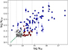 |
Fig. 1. C IV column density, log NCIV, versus the associated column density of neutral hydrogen, log NHI. The vertical dotted lines mark the values of log NHI = 13.0, 13.5, 14.0, and 14.8. Blue data points represent the detected C IV systems identified by D16; white triangles indicate the upper limits on log NCIV, which we used to derive the mock measurements (see Sect. 4.3). The red triangles represent the upper limits in the range between log NHI = 14.0 and log NHI = 14.8, not included in our tests. The dashed green line indicates the relation log NCIV = log NHI − 2.5 which is used, in the range 13 < log NHI < 14, to create the mock systems for one of our tests, see Sect. 4.3. |
3.2. Computation of the TPCF
The TPCF of the transmitted flux is computed, following Tie et al. (2022), as a function of the velocity separation between different pixels. Given two pixels with observed wavelengths λ1 and λ2, their wavelength separation can be converted into a velocity separation Δv using the following relation, derived from the Doppler effect (Eq. 3 in Perrotta et al. 2016), where c is the speed of light:
 (1)
(1)
Following Eq. 9 by Tie et al. (2022), the TPCF ξ can be written as
 (2)
(2)
where wi is the weight associated with pixel i, computed as the inverse of the square of the error associated with the flux value of pixel i. The TPCF is computed at the velocity separation Δv of pixels i and j. On the other hand, the flux overdensity δF of pixel i is defined as
 (3)
(3)
where Fi is the normalized flux of pixel i and  is the mean flux of the spectrum.
We computed the TPCF of the UVES deep spectrum of quasar HE0940-1050 considering the flux in the C IV forest, which corresponds to the wavelength range 540 − 623 nm. This interval corresponds to a velocity range of ∼42 600 km s−1: since our velocity grid is set at much smaller scales (up to 3500 km s−1), we do not miss out substantial information when computing the TPCF. With the goal of isolating the signal due to the weak C IV lines in mind, we also computed the TPCF by applying a process of ‘deabsorption’ of the metal lines to the spectrum of HE0940-1050. Lines were deabsorbed by subtracting the line model, obtained from the Voigt fitting in the context of Astrocook, from the sum of the spectral flux and the spectral continuum2. Uncertainties in the deabsorbed flux are the same as the original ones, as no error is associated with the line model. By deabsorbing the lines, we removed their contribution to the final TPCF result. All the TPCFs described in this paper are computed on a velocity grid ranging from 0 km s−1 to 3500 km s−1, with a bin size of 40 km s−1.
3.3. Computation of the uncertainties
Since we computed the TPCF for a single spectrum, we could not use the variance of the measurements (as in Tie et al. 2024) or bootstrapping techniques to estimate the error bars on the correlation function. Therefore, we determined the errors of the TPCF values by creating a set of N = 1000 mock spectra for each version of the spectrum that we considered, and we computed the TPCF on these mock spectra in order to obtain a distribution of the TPCF values for each velocity bin. Here we describe the procedure we used to create the mock spectra.
First, all absorption lines (C IV and other metal lines) are deabsorbed and a totally deabsorbed spectrum is created. Then, the absorption lines considered for the computation of the TPCF (see Section 4) are added to the deabsorbed spectrum with shuffled positions, which means that the same log N and b of the original systems are kept and only z is changed. In particular, lines that originally belonged to a doublet are no longer inserted as a doublet (e.g. C IV 1548 Å is considered as independent of C IV 1550 Å and assigned to a different position in the spectrum). In this way, we preserve the original flux but destroy all possible correlations between the systems, so that when computing the TPCF on the set of mock spectra, the plot will just show some random fluctuations around the zero level (i.e. noise), which we use to give an estimate of the errors. It is still possible to observe some spikes due to random correlations that originate after the shuffling, but these spikes are limited in number and do not affect the final distribution in a relevant way since the number of mock spectra is sufficiently high.
The creation of mock spectra was also performed with Astrocook, which allows mock Voigt profiles (based on a list of given parameters log N, b, and z) to be created and subsequently superimposes them on the spectrum. Once we computed the TPCF on all these samples of mock spectra, we took as error the region between the 16th and the 84th percentile of the distribution of the mock TPCFs in each velocity bin, which corresponds to an uncertainty of 1 σ. The 3 σ uncertainty was also computed from the distribution and considered in our analysis.
4. Results
4.1. TPCF of the complete spectrum
The TPCF computed with the complete spectrum is shown in Fig. 2. The two peaks that correspond to the velocity separation of the C IV doublet (at ∼500 km s−1) and of the Mg II doublet (at ∼770 km s−1) can be clearly seen in the plot, in addition to the peak at small velocity separations due to the structure of single lines or multi-component systems. Other peaks from other transitions (e.g. Si IV, which is also marked in the plot) are not evident. We also observe a significant anti-correlation in the large-scale regime, which is explained by the presence of very strong absorption systems in our spectrum, characterized by large, negative δF values, which anti-correlate with pixels at the continuum level.
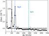 |
Fig. 2. TPCF computed on the complete spectrum, in black. The dashed vertical lines mark the velocity separation of the most common doublets: C IV (∼500 km s−1), which is the one we are interested in, but also Mg II (∼770 km s−1) and Si IV (∼1933 km s−1). The dark-grey and light-grey shaded regions indicate the uncertainties of 1 σ and 3 σ, respectively. |
We created a set of N = 1000 mock spectra by shuffling the position of both C IV and other metal transitions. In Fig. 2 we show the resulting 1 σ uncertainty as a shaded region, with a lighter shaded region indicating an uncertainty of 3 σ.
4.2. TPCF of the deabsorbed spectra
To isolate the contribution of the C IV associated with the IGM, we compared two versions of the spectrum in which we performed a partial C IV deabsorption. In the first case, we deabsorbed all the metal lines except for the 31 C IV lines associated with H I lines with log NHI < 14.8 (see Fig. 1). Then, we computed the TPCF on the resulting spectrum. According to the relation by Schaye (2001, see D16 for the details), a column density of log NHI = 14.8 corresponds at z ≃ 2.8 to an overdensity (δ + 1)≃11.8, which is generally assumed as the interface between CGM and IGM. However, as shown in Section 4.5, by applying this cut to C IV systems, the contribution from CGM absorbers is not entirely removed.
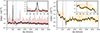 |
Fig. 3. TPCF for the spectrum where all metal lines have been deabsorbed except for C IV systems associated with log NHI < 14.8 (left) and log NHI < 14.0 (right) Lyα lines, plotted together with the 1 σ and 3 σ shaded regions obtained from the corresponding set of mock spectra. |
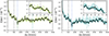 |
Fig. 4. Left: TPCF computed on the spectrum in which we included the mock measurements derived from the upper limits in addition to the C IV systems associated with log NHI < 14.0. Right: TPCF for the case in which we set the column density value of the mock C IV measurements such that log NCIV = log NHI − 2.5 in the range 13 < log NHI < 14. The shaded coloured regions indicate the 1 σ and 3 σ regions obtained from the distributions of the TPCF values computed on the corresponding sets of mock spectra. |
In the second case, we deabsorbed all the metal lines and only left the weakest C IV systems, namely those associated with H I lines with log NHI < 14.0, which are seven systems in total. The TPCF was then also computed on this version of the spectrum. A column density of log NHI = 14.0 at z = 2.8 is translated into an overdensity of (δ + 1)≃3.0, typical of the intergalactic environment, as we confirm in Section 4.5. In both cases, we determined the uncertainties on the TPCF as described in Sections 3.3 and 4.1, and we only distributed the C IV lines used for the computation of the respective TPCF over the totally deabsorbed spectra.
The two resulting TPCFs are shown in Fig. 3. In the former case, the C IV peak is visible and significant (i.e. out of the 3 σ level), while in the latter case the TPCF does not show a significant peak at the velocity separation of the C IV doublet.
4.3. TPCF of the deabsorbed spectra with mock weak systems
In Fig. 3 we show that when we deabsorb all metal lines and only leave the C IV associated with H I systems with log NHI < 14.0, there is no significant signal of IGM enrichment in the TPCF of the flux. Since there are seven weak C IV systems left in the spectrum after the deabsorption, this result suggests that the sensitivity of the TPCF technique, when applied to a real spectrum, is limited.
To further test the sensitivity threshold of the method, we considered as detections the 3 σ upper limits on the C IV column density determined by D16 at the redshift of the H I lines with 13.5 ≤ log NHI < 14.0 (see Table 1 and the white triangles in Fig. 1). Using Astrocook, we created 46 mock C IV Voigt profiles from the upper limits assuming a Doppler parameter b = 7 km s−1 and we added them to the version of the spectrum with the weak C IV systems associated with log NHI < 14.0. The TPCF determined from this spectrum with the associated uncertainties is shown in Fig. 4 (left). In this case as well, the peak at 500 km s−1 is not significant.
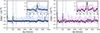 |
Fig. 5. Left: TPCF computed on the synthetic spectrum (with same S/N as the original one) in which we included the C IV systems associated with log NHI < 14.0. Right: TPCF for the case in which we also added the 135 mock measurements derived from Eq. (4) in addition to the weak systems. The shaded coloured regions indicate the 1 σ and 3 σ uncertainty regions obtained from the distributions of TPCF values computed on the corresponding sets of mock spectra. |
As a final test, we adopted the procedure described in Ellison et al. (2000) to account for the metal enrichment also associated with Lyα lines with column densities of 13 < log NHI < 13.5 (89 lines in total), for which D16 did not compute the C IV upper limits. We assumed the following relation between column densities:
 (4)
(4)
and applied it to all Lyα lines with 13.0 < log NHI < 14.0 (135 lines, see Fig. 1), except those with a detected C IV absorption. Mock C IV lines were generated assuming b = 7 km s−1 and distributed on the spectrum with deabsorption at log NHI > 14.0. Finally, we computed the TPCF on the resulting spectrum and created the related set of N = 1000 mock spectra, shuffling the lines as usual. The resulting TPCF and associated uncertainty region is shown in Fig. 4 (right). The peak is still within the shaded region, and therefore is not significant.
4.4. TPCF of the synthetic spectra with weak systems
Another test we did to determine the sensitivity of the TPCF technique was to create synthetic spectra in which we inserted the extremely weak systems. This test is similar to the one described in the previous section, with the difference that we did not use the original spectrum: we created a synthetic spectrum that has the same S/N of the original totally deabsorbed one, but with gaussian distributed noise added to each pixel (this step was also performed with Astrocook). Then, we added the C IV systems associated with log NHI < 14.0 in one case, and added the 135 mock systems (with column densities following Eq. (4)) in another case. In a sense, these two tests are analogous to Fig. 3, right, and Fig. 4, right, but with the use of a synthetic spectrum, which allows us to remove the spurious signal that remains in the original flux in order to highlight the strength of the C IV peak that originates from the weak systems. This test is useful in order to understand how relevant the spectral features are in shaping the correlation function and see how the results change when we remove these features by mocking an ‘ideal deabsorption’. On the other hand, we also remove the possible signature of IGM enrichment present below the detection limit.
The resulting TPCFs are shown in Fig. 5. Results show a non-significant C IV peak in the former case (Fig. 5, left), but a significant one (at a 3 σ level) when we add the 135 mock measurements (Fig. 5, right). This suggests that the spectral features can considerably contaminate the TPCF signal and prevent the detection of the weak systems, since this peak is not recorded by the previous test in Fig. 4, right. We also observe a significant peak at Δv ∼ 3180 km s−1, which we verified is due to the presence of the four weak C IV doublets at z ≃ 2.85796, 2.89872, 2.940455, and 2.98251 with relative separations: Δv ≃ 3150, 3192 and 3182 km s−1, respectively.
4.5. Flux probability distribution function
In addition, we computed the flux decrement probability distribution function (PDF) in log10-unit, following the equation by Tie et al. (2022):
 (5)
(5)
where frac(a, b) is the fraction of pixels with log10(1 − F) values between a and b.
Hennawi et al. (2021) and Tie et al. (2022) use this distribution to identify the pixels in the C IV forest associated with the CGM and mask them. Indeed, the CGM is expected to be associated with the strongest C IV absorptions and therefore with the tail of the PDF at large 1 − F values.
We checked the effects of our deabsorptions at different H I column density thresholds on the PDF of the flux decrement. Figure 6 shows in black the PDF of the flux for the original spectrum with a clear tail extending to high values of 1 − F. We then computed the PDF for the spectrum with only C IV associated with log NHI < 14.8 (red line) and with log NHI < 14.0 (orange line). In blue, we also show the PDF corresponding to the synthetic spectrum in Fig. 5, left. We notice that when we deabsorb at log NHI = 14.8 (red line), the CGM contamination is still present; on the other hand, the deabsorption at log NHI = 14.0 (orange and blue lines) removes the CGM absorbers effectively.
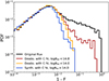 |
Fig. 6. Flux PDF of four different versions of the spectrum: the original one (with no deabsorption, in black); the version with only C IV systems associated with log NHI < 14.8 (red); the one with only C IV systems associated with log NHI < 14.0 (orange); the synthetic spectrum with weak C IV systems (log NHI < 14.0) and the same S/N as the original one (blue). |
We specify that the exact shape and normalization of the flux decrement PDF, and the value of 1 − F at which there is the transition between IGM and CGM, may depend on the specific enrichment model adopted by Tie et al. (2022). However, since the shape and values of our PDF are qualitatively consistent with the theoretical predictions, we consider it as a further empirical tool to identify the IGM-CGM transition.
5. Summary and discussion
In this paper, we analysed the ultra-high S/N and high-resolution spectrum of the quasar HE0940-1050 (zem = 3.0932), obtained with the VLT-UVES spectrograph, with the goal of detecting the IGM metal enrichment by computing the TPCF between the flux overdensities associated with the pixels, with a specific focus on the C IV forest region at 2.51 ≲ z ≲ 3.02 (corresponding to the wavelength interval 540 - 623 nm). First, we identified and fitted Voigt profiles to the C IV doublets and all the other metal absorption lines in the region of the spectrum redward of the Lyα emission of the quasar. Then, we computed the TPCF in the window 540–623 nm, for the following cases:
-
Original spectrum;
-
Spectrum deabsorbed of all metal lines except for the 31 C IV lines associated with Lyα lines with log NHI < 14.8;
-
Spectrum deabsorbed of all metal lines except for the seven weak C IV lines associated with Lyα lines with log NHI < 14.0;
-
Same as iii., but with the addition of 46 mock measurements derived from the upper limits on log NCIV derived by D16;
-
Same as iii., but also including 135 mock measurements associated with the Ly-α lines with 13.0 < log NHI < 14.0 and such that log NCIV = log NHI − 2.5 and b = 7 km s−1;
-
Same as iii. but with a synthetic spectrum with the same S/N (gaussian distributed) as the totally deabsorbed complete spectrum;
-
Same as v. but using a synthetic spectrum with the same S/N (gaussian distributed) as the totally deabsorbed complete spectrum.
For each of these cases, to estimate the errors associated with the TPCF values, we created a set of 1000 mock spectra by shuffling the position of the absorption lines that are left after the deabsorption procedure. In case i. (Fig. 2), the C IV and Mg II peaks are clearly visible. We also observe the expected enhanced correlation on small separations due to the velocity structure of the single absorption systems (Tie et al. 2024), and its flattening at large velocity separations.
In Fig. 6, we show that by applying the two different cuts (case ii. and iii.) on the associated log NHI, we gradually remove from the PDF the contribution from the strong CGM absorbers, which are responsible for the flatness of the function at large 1 − F values, until we only keep the weak IGM absorbers, which do not produce large flux decrements and therefore make the PDF drop at large 1 − F values (Hennawi et al. 2021; Tie et al. 2022). In particular, the PDF shows that only deabsorbing the C IV systems associated with log NHI > 14.8 (red line, corresponding to Fig. 3, left) is not sufficient to remove the CGM contribution, which still creates the flatness. We need to deabsorb more systems (orange line, corresponding to Fig. 3, right) in order to isolate the IGM signal. In other words, in case ii., where the C IV peak is significant at 3 σ, we are still affected by the systems associated with the CGM. On the other hand, when we deabsorb even more C IV systems (case iii.) and are left with the IGM contribution only, the C IV peak is found to be consistent with the noise level (Fig. 3, right).
Figure 4 shows that the TPCF is not responsive to the presence of additional 135 weak mock C IV systems with which we further enriched the spectrum. This suggests a lack of sensitivity related to systems associated with typical IGM column densities, log NHI < 14.0.
The TPCFs in Fig. 3 and Fig. 4 show a signal on scales smaller than ∼800 km s−1, which we ascribe to the presence of residual flux after deabsorption and weak correlations in the noise structure. Indeed, when we use a synthetic spectrum in cases vi. and vii. (Fig. 5), the spurious signal disappears and the C IV peaks due to the weak absorptions become visible. It is not clear whether applying the method to a larger sample would average out this spurious signal, which is always expected on small scales.
Finally, we can derive qualitative constraints on the IGM metal enrichment from the comparison of our results based on the synthetic spectrum with those obtained by Tie et al. (2022) with noiseless spectra from simulations. Contrasting our Fig. 5 with their Fig. 5, which shows the predictions they obtain for a resolution comparable to the UVES one (full width at half maximum = 10 km s−1), we can state the following:
-
Assuming a minimum mass for the haloes of log Mmin = 9.50 M⊙, and a radius of the enriched bubble (enrichment radius) of R = 0.50 cMpc, our result is consistent with a metallicity [C/H] ∼ −3.80;
-
On the other hand, considering R = 0.50 cMpc and assuming [C/H] = −3.50, we can estimate the minimum mass of the halo to be between log Mmin = 10 and 11 M⊙;
-
Finally, in the case of a minimum mass of log Mmin = 9.50 M⊙ and a metallicity [C/H] ∼ −3.50, our result indicates bubbles with a radius R < 0.50 cMpc.
The overall qualitative picture that emerges from this comparison is that if we assume a metallicity of [C/H] ∼ −3.50, the volume filling factor of the enriched regions predicted by the simple model by Tie et al. (2022) to reproduce our TPCF is on the order of 5 percent or less. This is somewhat in contradiction with the result obtained by D16 (who also adopt simple assumptions) where the volume filling factor of IGM gas enriched to a metallicity log Z/Z ≳ −3.0 is derived to be ∼10 − 13 percent. More detailed hydrodynamical simulations of the early chemical enrichment should be used to compare with observations and derive constraints on the metal enrichment of the IGM.
In conclusion, with our study of a single line of sight at high resolution and very high S/N, we show that, although very weak C IV systems (log NCIV ∼ 11.5) are present and detected by eye, their presence is not recorded by the TPCF technique. However, systems with column densities lower than log NCIV ∼ 11.7 were not successfully recorded with the stacking method in Ellison et al. (2000) either, which confirms the fact that the search for weak systems is a challenging task to pursue with even a very high S/N spectrum. We expect the results to improve when applying the same method to a larger sample of bright quasar spectra. However, residual correlations due to imperfections in the data reduction and analysis could affect the region of the C IV peak and wash out the result even when multiple lines of sight are considered. We plan to extend the same procedure applied in this work to a larger sample of quasar spectra in a forthcoming paper.
Data availability
Tables 1 and 2 are available at the CDS via https://cdsarc.cds.unistra.fr/viz-bin/cat/J/A+A/705/A16.
Acknowledgments
We are grateful to the anonymous referee for their comments, which have been useful to improve the quality of the paper. We would like to thank Louise Welsh and Vid Irsic for helpful discussions. This paper is based on observations collected at the European Southern Observatory Very Large Telescope, Cerro Paranal, Chile – Programs 65.O-0474, 166.A-0106, 079.B-0469, 185.A-0745, 092.A-0170 and 092.A-0770.
References
- Becker, G. D., Bolton, J. S., & Lidz, A. 2015, PASA, 32 [Google Scholar]
- Cen, R., & Chisari, N. E. 2011, ApJ, 731, 11 [NASA ADS] [CrossRef] [Google Scholar]
- Cupani, G., D’Odorico, V., Cristiani, S., et al. 2020, in Software and Cyberinfrastructure for Astronomy VI, eds. J. C. Guzman, & J. Ibsen, SPIE Conf. Ser., 11452, 114521U [Google Scholar]
- D’Odorico, V., Cristiani, S., Pomante, E., et al. 2016, MNRAS, 463, 2690 [Google Scholar]
- Ellison, S. L., Songaila, A., Schaye, J., & Pettini, M. 2000, AJ, 120, 1175 [NASA ADS] [CrossRef] [Google Scholar]
- Hennawi, J. F., Davies, F. B., Wang, F., & Oñorbe, J. 2021, MNRAS, 506, 2963 [NASA ADS] [CrossRef] [Google Scholar]
- Karaçaylı, N. G., Martini, P., Weinberg, D. H., et al. 2023, MNRAS, 522, 5980 [Google Scholar]
- Madau, P., Ferrara, A., & Rees, M. J. 2001, ApJ, 555, 92 [Google Scholar]
- Murphy, M. 2016a, UVESheadsort: UVESheadsort: VLT/UVES pipeline preparation [Google Scholar]
- Murphy, M. 2016b, UVESpopler: Version 0.71 release [Google Scholar]
- Murphy, M. T., Kacprzak, G. G., Savorgnan, G. A. D., & Carswell, R. F. 2019, MNRAS, 482, 3458 [NASA ADS] [CrossRef] [Google Scholar]
- Péroux, C., & Howk, J. C. 2020, ARA&A, 58, 363 [CrossRef] [Google Scholar]
- Perrotta, S., D’Odorico, V., Prochaska, J. X., et al. 2016, MNRAS, 462, 3285 [NASA ADS] [CrossRef] [Google Scholar]
- Schaye, J. 2001, ApJ, 559, 507 [NASA ADS] [CrossRef] [Google Scholar]
- Schaye, J., Aguirre, A., Kim, T.-S., et al. 2003, ApJ, 596, 768 [Google Scholar]
- Shen, S., Madau, P., Aguirre, A., et al. 2012, ApJ, 760, 50 [NASA ADS] [CrossRef] [Google Scholar]
- Shen, S., Madau, P., Guedes, J., et al. 2013, ApJ, 765, 89 [NASA ADS] [CrossRef] [Google Scholar]
- Tie, S. S., Hennawi, J. F., Kakiichi, K., & Bosman, S. E. I. 2022, MNRAS, 515, 3656 [Google Scholar]
- Tie, S. S., Hennawi, J. F., Wang, F., et al. 2024, MNRAS, 535, 223 [Google Scholar]
The overdensity is defined as  , where ρ is the mass density and
  the cosmic mean mass density.
Another possibility to deabsorb the spectral lines would be to divide the flux by the line model, but we prefer to subtract it in order to avoid spikes when the flux and the model go to zero.
Appendix A: Additional figures
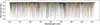 |
Fig. A.1. The UVES deep spectrum (original version, no deabsorption), normalized to the continuum. Coloured lines show an example of 50 mock spectra taken from the related set of 1000 mock spectra used to estimate the uncertainties on the TPCF. |
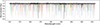 |
Fig. A.2. The version of the UVES deep spectrum in which we deabsorbed all metal absorption lines and C IV doublets associated with log NHI > 14.8, in black, with coloured lines showing an example of 50 out of the 1000 mock spectra created for this version of the spectrum. |
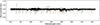 |
Fig. A.3. Similar to Fig. A.2 and Fig. A.1, but showing the case in which we left only C IV associated with log NHI < 14.0, in black, with an example of 50 mock spectra taken from the related set of mock spectra (coloured lines). |
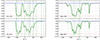 |
Fig. A.4. An example of a C IV system and a Mg II system found in the complete spectrum and fitted with the use of Astrocook. The green line indicates the line models (Voigt fitting), the vertical dashed lines are used to mark the different components. |
All Figures
|
Fig. 1. C IV column density, log NCIV, versus the associated column density of neutral hydrogen, log NHI. The vertical dotted lines mark the values of log NHI = 13.0, 13.5, 14.0, and 14.8. Blue data points represent the detected C IV systems identified by D16; white triangles indicate the upper limits on log NCIV, which we used to derive the mock measurements (see Sect. 4.3). The red triangles represent the upper limits in the range between log NHI = 14.0 and log NHI = 14.8, not included in our tests. The dashed green line indicates the relation log NCIV = log NHI − 2.5 which is used, in the range 13 < log NHI < 14, to create the mock systems for one of our tests, see Sect. 4.3. |
| In the text | |
|
Fig. 2. TPCF computed on the complete spectrum, in black. The dashed vertical lines mark the velocity separation of the most common doublets: C IV (∼500 km s−1), which is the one we are interested in, but also Mg II (∼770 km s−1) and Si IV (∼1933 km s−1). The dark-grey and light-grey shaded regions indicate the uncertainties of 1 σ and 3 σ, respectively. |
| In the text | |
|
Fig. 3. TPCF for the spectrum where all metal lines have been deabsorbed except for C IV systems associated with log NHI < 14.8 (left) and log NHI < 14.0 (right) Lyα lines, plotted together with the 1 σ and 3 σ shaded regions obtained from the corresponding set of mock spectra. |
| In the text | |
|
Fig. 4. Left: TPCF computed on the spectrum in which we included the mock measurements derived from the upper limits in addition to the C IV systems associated with log NHI < 14.0. Right: TPCF for the case in which we set the column density value of the mock C IV measurements such that log NCIV = log NHI − 2.5 in the range 13 < log NHI < 14. The shaded coloured regions indicate the 1 σ and 3 σ regions obtained from the distributions of the TPCF values computed on the corresponding sets of mock spectra. |
| In the text | |
|
Fig. 5. Left: TPCF computed on the synthetic spectrum (with same S/N as the original one) in which we included the C IV systems associated with log NHI < 14.0. Right: TPCF for the case in which we also added the 135 mock measurements derived from Eq. (4) in addition to the weak systems. The shaded coloured regions indicate the 1 σ and 3 σ uncertainty regions obtained from the distributions of TPCF values computed on the corresponding sets of mock spectra. |
| In the text | |
|
Fig. 6. Flux PDF of four different versions of the spectrum: the original one (with no deabsorption, in black); the version with only C IV systems associated with log NHI < 14.8 (red); the one with only C IV systems associated with log NHI < 14.0 (orange); the synthetic spectrum with weak C IV systems (log NHI < 14.0) and the same S/N as the original one (blue). |
| In the text | |
|
Fig. A.1. The UVES deep spectrum (original version, no deabsorption), normalized to the continuum. Coloured lines show an example of 50 mock spectra taken from the related set of 1000 mock spectra used to estimate the uncertainties on the TPCF. |
| In the text | |
|
Fig. A.2. The version of the UVES deep spectrum in which we deabsorbed all metal absorption lines and C IV doublets associated with log NHI > 14.8, in black, with coloured lines showing an example of 50 out of the 1000 mock spectra created for this version of the spectrum. |
| In the text | |
|
Fig. A.3. Similar to Fig. A.2 and Fig. A.1, but showing the case in which we left only C IV associated with log NHI < 14.0, in black, with an example of 50 mock spectra taken from the related set of mock spectra (coloured lines). |
| In the text | |
|
Fig. A.4. An example of a C IV system and a Mg II system found in the complete spectrum and fitted with the use of Astrocook. The green line indicates the line models (Voigt fitting), the vertical dashed lines are used to mark the different components. |
| In the text | |
Current usage metrics show cumulative count of Article Views (full-text article views including HTML views, PDF and ePub downloads, according to the available data) and Abstracts Views on Vision4Press platform.
Data correspond to usage on the plateform after 2015. The current usage metrics is available 48-96 hours after online publication and is updated daily on week days.
Initial download of the metrics may take a while.