| Issue |
A&A
Volume 705, January 2026
|
|
|---|---|---|
| Article Number | A66 | |
| Number of page(s) | 11 | |
| Section | The Sun and the Heliosphere | |
| DOI | https://doi.org/10.1051/0004-6361/202556276 | |
| Published online | 07 January 2026 | |
Quasi-biennial oscillations and Rieger-type periodicities in a Babcock–Leighton solar dynamo
1
Physics and Astronomy Department, University of Florence (FI), 50019, Italy
2
Indian Institute of Astrophysics, Koramangala, Bengaluru, 560034
India
3
University College of Science and Technology, Department of Chemical Technology, University of Calcutta, 92, A.P.C. Road, Kolkata, 700009 West Bengal, India
4
Department of Physics, Indian Institute of Technology (BHU), Varanasi, 221005
India
★ Corresponding author: This email address is being protected from spambots. You need JavaScript enabled to view it.
Received:
6
July
2025
Accepted:
24
October
2025
Abstract
Context. The Sun’s magnetic field exhibits the 11 year solar cycle as well as shorter periodicities, popularly known as the quasi-biennial oscillations (QBOs) and Rieger-type periods. Although several theories have been proposed to explain the origin of QBOs and Rieger-type periods, no single theory has had widespread acceptance.
Aims. We explore whether the Babcock–Leighton dynamo can produce Rieger-type periodicity and QBOs and investigate their underlying physical mechanisms.
Methods. We used the observationally guided 3D kinematic Babcock–Leighton dynamo model, which has emerged as a successful model for reproducing many characteristic features of the solar cycle. We used Morlet wavelet and global wavelet power spectrum techniques to analyze the data obtained from the model.
Results. In our model, we report QBOs and Rieger-type periods for the first time. Further, we investigated the individual Babcock–Leighton parameters (fluctuations in flux, latitude, time delay, and tilt scatter) role in the occurrence of QBOs and Rieger-type periods. We find that while fluctuations in the individual parameters of the Babcock–Leighton process can produce QBOs and Rieger-type periodicity, their occurrence probability is enhanced when considering combined fluctuations of all parameters in the Babcock–Leighton process. Finally, we find that with the increase in dynamo supercriticality, the model tends to suppress the generation of Rieger-type periodicity. Thus, this result supports earlier studies that suggest the solar dynamo is not highly supercritical.
Conclusions. The Babcock–Leighton dynamo model successfully reproduces QBOs and Rieger-type periodicities that are observed in various solar activity data.
Key words: dynamo / methods: data analysis / Sun: magnetic fields / Sun: oscillations / sunspots
© The Authors 2026
 Open Access article, published by EDP Sciences, under the terms of the Creative Commons Attribution License (https://creativecommons.org/licenses/by/4.0), which permits unrestricted use, distribution, and reproduction in any medium, provided the original work is properly cited.
This article is published in open access under the Subscribe to Open model. This email address is being protected from spambots. You need JavaScript enabled to view it. to support open access publication.
1. Introduction
The global solar magnetic field shows cyclic variation in its activity levels with an average period of 11 years (or 22 years when considering the polarity). Beyond this 11 year oscillation, there are long-term modulations, which are best seen in the sunspot number or its proxies (10Be and 14C; Usoskin 2023), such as the ∼90 year Gleissberg cycle (Gleissberg 1939), the ∼210 year Suess cycle (Suess 1980), and the Grand minimum (like the Maunder minimum; Eddy 1976). In addition to these long-term modulations and variations in periodicities and amplitude, the solar cycle shows Rieger-type periodic variations (< 1 year), which are so-called bursts of activity or seasons of the Sun (Rieger et al. 1984; McIntosh et al. 2015). In addition to these Rieger-type periodicities, several mid-range periodicities have been observed between 1 and 11 years, known as quasi-biennial oscillations (QBOs; Bazilevskaya et al. 2000; Ruzmaikin et al. 2008; Vecchio & Carbone 2009; Chowdhury et al. 2022; Ravindra et al. 2022). Studies suggest that QBOs attain their highest amplitude during solar maxima and become weaker during the minimum phase of the solar cycle; thus, the amplitude of the QBO signals is in phase with the 11 year solar cycle. Moreover, QBOs develop in both hemispheres independently with variable periodicity (Bazilevskaya et al. 2014; Jain et al. 2023) and show asymmetry, intermittent behavior, and presence in only a few hemispheric cycles of sunspot number (Ravindra et al. 2022).
There is extensive literature available on the origin of QBOs and Rieger-type periodicities in solar activity. However, the conclusions of different authors on the origin of these periodicities differ. The majority of authors suggest that QBOs arise intrinsically from the solar dynamo process, which itself drives the 11 year solar cycle (e.g., Benevolenskaya 1998; Howe et al. 2000; Knaack & Stenflo 2005; Ruzmaikin et al. 2008; Cho et al. 2014; Inceoglu et al. 2019). Well-known explanations have been given for Rieger-type periodicity and QBOs, including a two-dynamo process, in which one operates near the solar surface and the other at the base of the convection zone (CZ) (Käpylä et al. 2016); instabilities of magnetic Rossby waves in the solar tachocline (Chowdhury et al. 2009; Zaqarashvili et al. 2010; Korsós et al. 2023); beating between dipolar and quadrupolar magnetic field configurations generated by the solar dynamo (Simoniello et al. 2013); and the typical lifetimes of complex active regions (Chowdhury et al. 2013). Moreover, Dikpati et al. (2018, 2021) suggested that the nonlinear oscillations in the tachocline might be responsible for the emergence of QBOs and Rieger-type periodicities. They also provided a quantitative physical mechanism for forecasting the strength and duration of the bursty seasons or seasons of the Sun several months in advance (Dikpati et al. 2017). Furthermore, the results of magnetohydrodynamics (MHD) numerical simulations (Karak et al. 2015; Käpylä et al. 2016; Strugarek et al. 2018) also show the existence of two-cycle modes with longer and shorter periods, and researchers believe that this may also be a possible candidate for an explanation of Rieger-type periodicities.
The solar magnetic field and its cycle-to-cycle variations are believed to be the result of the dynamo process, which operates in the solar convection zone (SCZ). Dynamo is a cyclic process in which toroidal and poloidal fields support each other. In the classical αΩ-type dynamo, the helical α generates the poloidal field from the toroidal field, while the Ω effect produces the toroidal field from the poloidal one through differential rotation (Parker 1955; Steenbeck et al. 1966). Under certain conditions, this cyclic process continues and sustains the long-term evolution of the solar magnetic field. However, in recent years, observational studies (Dasi-Espuig et al. 2010; Kitchatinov & Olemskoy 2011; Mordvinov et al. 2022; Cameron & Schüssler 2023) suggest that the decay and dispersal of tilted bipolar magnetic regions (BMRs) on the solar surface generate the poloidal field, popularly known as the Babcock–Leighton mechanism (Babcock 1961; Leighton 1969). In recent decades, Babcock–Leighton-type dynamo models, which involve the Babcock–Leighton mechanism in solar polar field generation, have emerged as a popular paradigm for explaining various key features of the observed solar magnetic field, including polarity reversals and double peaks (Gnevyshev 1977; Karak et al. 2018; Mordvinov et al. 2022); solar cycle prediction (Hazra & Choudhuri 2019; Petrovay 2020; Kumar et al. 2021a, 2022); poleward migration of surface magnetic field; equatorward migration of the toroidal field; and solar cycle variability (Karak et al. 2014; Charbonneau 2020; Karak 2023; Kumar et al. 2024). The key strength of Babcock–Leighton models is that it has strong observational support for the toroidal-to-poloidal field conversion part of the model, and in the model, we can include fluctuations in BMR properties, which are observable and quantifiable (Jiang et al. 2014a; Cameron & Schüssler 2023; Sreedevi et al. 2024). These characteristics enable the models to reproduce and explain various observed and irregular features of the solar magnetic cycles.
Although the Babcock–Leighton dynamo model successfully reproduces many observed features of the solar magnetic field, some characteristics remain unexplained. For example, Inceoglu et al. (2019) found that a 2D turbulent α effect dynamo model is capable of generating QBOs; however, the 2D Babcock–Leighton dynamo model fails to reproduce these features. They suggested that in the turbulent α dynamo model, the Lorentz force provides a feedback mechanism on the flow fields, which enables the model to generate QBOs.
In this work, we explore whether the Babcock–Leighton dynamo can produce Rieger-type periodicity and QBOs and the underlying physical mechanism. We used a 3D kinematic Babcock–Leighton dynamo model, STABLE (Surface Flux Transport And Babcock–LEighton; Miesch & Dikpati 2014). The STABLE model captures the BMR properties more realistically and makes a close connection between the model and observation. In the Babcock–Leighton process, the poloidal field was generated through the decay and dispersal of tilted BMRs. Therefore, BMR properties are crucial in the Babcock–Leighton mechanism. We focus on the various fluctuating parameters in the Babcock–Leighton process caused by turbulent convection (Kumar et al. 2024). Specifically, we investigate the roles of four key BMR properties, which include fluctuations in (i) the tilt angle, (ii) the flux, (iii) the time delay of emergence, and (iv) the emergence latitude.
The structure of this paper is as follows. In Section 2, we describe our model and how we implemented it to generate the sunspot cycle and surface magnetic field. Section 3 outlines the methodology adopted to analyze the model data, and in Section 4, we present and discuss the results obtained from the dynamo model. The last section presents the conclusions of this study.
2. Model
To understand and demonstrate QBOs and Rieger-type periods, we performed our study using the 3D Babcock–Leighton dynamo model, STABLE (Miesch & Teweldebirhan 2016). The Babcock–Leighton process involves stochastic fluctuations and nonlinearity and is responsible for generating the Sun’s poloidal magnetic field through the decay and dispersal of tilted BMRs on the solar surface. This poloidal field eventually gives rise to the toroidal field through differential rotation and produces new BMRs via magnetic buoyancy, thereby leading to the sunspot cycle. In the STABLE model, BMRs are deposited on the surface based on the toroidal field present in the CZ. The model’s BMR prescriptions are specified from observations. Thus, this model produces observed features of the solar magnetic field reasonably well (Miesch & Dikpati 2014; Miesch & Teweldebirhan 2016), including the correct latitude dependence of the polar field: higher latitudes of BMR emergence correspond to less polar field generation (Kumar et al. 2024), latitude quenching (Karak 2020), polar rush, triple reversal (Mordvinov et al. 2022), and irregular cycles and grand minima (Karak & Miesch 2017, 2018). The details of the model used in this study are described below.
The STABLE dynamo model was originally developed by Mark Miesch (Miesch & Dikpati 2014; Miesch & Teweldebirhan 2016) and improved by Karak & Miesch (2017) to make a close connection of BMR eruptions with observations. It realistically captures the Babcock–Leighton process using the available surface observation of BMRs and large-scale flows such as meridional circulation and differential rotation. In this model, we solved the induction equation in spherical coordinates (r, θ, ϕ) for the whole SCZ:
![Mathematical equation: $$ \begin{aligned} \frac{\partial \boldsymbol{B}}{\partial t} = \boldsymbol{\nabla \times } \left[ (\boldsymbol{V} +\boldsymbol{\gamma }) \times \boldsymbol{B} - \eta _t \boldsymbol{\nabla \times } \boldsymbol{B} \right], \end{aligned} $$](/articles/aa/full_html/2026/01/aa56276-25/aa56276-25-eq1.gif) (1)
(1)
with 0.69 R⊙ ≤ r ≤ R⊙, where R⊙ is the solar radius, 0 ≤ θ ≤ π and 0 ≤ ϕ ≤ 2π. In this study, the model used is a kinematic Babcock–Leighton dynamo in which V is the velocity field:
 (2)
(2)
where vr and vθ are the components of the axisymmetric meridional flow and (Ω = vϕ/r sin θ) is the differential rotation. For meridional circulation, we considered the single-cell circulation profile, which closely resembles surface observations (Rajaguru & Antia 2015; Gizon et al. 2020) and was used earlier in Karak & Cameron (2016), Karak & Miesch (2017), Kumar et al. (2024). Near the surface, we considered the meridional flow speed to be 20 m s−1 toward the pole; near the base of the CZ, the flow is 2 m s−1 and smoothly decreasing to zero at the lower boundary (0.69 R⊙) of CZ. The differential rotation (Ω) profile used in this model roughly captures the observed properties as inferred by helioseismology (Schou et al. 1998).
In the Induction Equation (1), γ represents magnetic pumping, which helps to suppress the loss of toroidal flux through the surface due to diffusivity. In this model, we consider radially downward magnetic pumping of speed 20 m s−1 in the near-surface layer of the Sun (r ≥ 0.9 R⊙); see equation (3) of Karak & Miesch (2017). Magnetic pumping makes our Babcock–Leighton dynamo models consistent with the surface flux transport (SFT) model (Cameron & Schüssler 2012; Kumar et al. 2024). Moreover, the magnetic pumping helps our model to produce an 11 year magnetic cycle at very high turbulent diffusivity as inferred in the observations (on the order of 1012 cm2 s−1) (Karak & Cameron 2016). Next, we considered an effective radial-dependent turbulent diffusivity represented by ηt in Equation (1) such that
![Mathematical equation: $$ \begin{aligned} \eta _t(r)&= \eta _{RZ} + \frac{\eta _{cz}}{2}\left[1 + \mathrm{erf} \left(\frac{r - 0.715\,R_{\odot }}{0.0125\,R_{\odot }}\right) \right] \\ \nonumber&\quad +\frac{\eta _{\mathrm{surf} }}{2}\left[1 + \mathrm{erf} \left(\frac{r - 0.956\,R_{\odot }}{0.025\,R_{\odot }}\right) \right], \end{aligned} $$](/articles/aa/full_html/2026/01/aa56276-25/aa56276-25-eq3.gif)
where ηRZ = 109 cm2 s−1, ηsurf = 4.5 × 1012 cm2 s−1, and ηcz = 1.5 × 1012 cm2 s−1.
We note that this model does not capture full magnetohydrodynamics in the convection, so the BMRs do not appear automatically. This model has a prescription known as the SpotMaker algorithm for this mechanism (Miesch & Teweldebirhan 2016). First, it computes the spot-producing toroidal field strength near the base of the CZ in a hemisphere presented as
 (3)
(3)
where ra = 0.7 R⊙, rb = 0.715 R⊙ (R⊙ is the radius of the Sun) and h(r) = h0(r − ra)(rb − r), h0 is a normalization factor. Furthermore, the model places a BMR on the solar surface only when certain conditions are satisfied. First,  must exceed a critical magnetic field strength value Btc(θ). The critical magnetic field Btc depends on latitude, making the emergence of BMR difficult at higher latitudes such that
![Mathematical equation: $$ \begin{aligned} B_{tc}(\theta )&= B_{t0} \exp \left[ \beta (\theta - \pi /2) \right] \ \ \ \ \ \ \mathrm{{for}}\ \ \ \ \theta > \pi /2, \nonumber \\&= B_{t0} \exp \left[ \beta (\pi /2 - \theta ) \right]\ \ \ \ \ \ \ \ \mathrm{{for}}\ \ \ \ \theta \le \pi /2, \end{aligned} $$](/articles/aa/full_html/2026/01/aa56276-25/aa56276-25-eq6.gif) (4)
(4)
where Bt0 is 2 kG and β = 5. This latitude-dependent BMR eruption plays an important role in capturing latitude-dependent quenching (Petrovay 2020; Jiang 2020; Karak 2020) and helps the model reproduce BMRs consistent with observations (Solanki et al. 2008; Mandal et al. 2017). Our model produces the first BMR when  . Then, after a time interval dt following the first BMR eruption, the model can produce the next BMR only when these two conditions are satisfied:
-
(i)
-
(ii)
dt ≥ Δ.
Here, Δ is the time delay between two consecutive BMR eruptions and follows a lognormal distribution obtained from the fitting of observed sunspots:
![Mathematical equation: $$ \begin{aligned} P(\Delta ) = \frac{1}{\sigma _d\Delta \sqrt{2\pi }}\mathrm{{exp}}\left[\frac{-(\ln \Delta - \mu _d)^2}{2\sigma _d^2}\right], \end{aligned} $$](/articles/aa/full_html/2026/01/aa56276-25/aa56276-25-eq9.gif) (5)
(5)
where σd and μd are specified as ![Mathematical equation: $ \sigma_d^2=\frac{2}{3}\left[\ln\tau_s - \ln\tau_p\right] $](/articles/aa/full_html/2026/01/aa56276-25/aa56276-25-eq10.gif) and μd = σd2 + lnτp. Here, Δ represents the time delay between two successive BMRs (normalized to one day). The values τp = 0.8 days and τs = 1.9 days were obtained from observed solar maxima data. Since observations suggest the time delay of BMR eruptions to be solar cycle phase-dependent (Jiang et al. 2018), we consider τp and τs to be magnetic-field-dependent such that
and μd = σd2 + lnτp. Here, Δ represents the time delay between two successive BMRs (normalized to one day). The values τp = 0.8 days and τs = 1.9 days were obtained from observed solar maxima data. Since observations suggest the time delay of BMR eruptions to be solar cycle phase-dependent (Jiang et al. 2018), we consider τp and τs to be magnetic-field-dependent such that
![Mathematical equation: $$ \begin{aligned} \tau _p = \frac{2.2}{1 + \left[\frac{B_b}{B_0}\right]^2}\,\mathrm{{days}}, \ \ \ \ \mathrm{{and}}\ \ \ \ \tau _s = \frac{20}{1 + \left[\frac{B_b}{B_0}\right]^2}\,\mathrm{{days}}, \end{aligned} $$](/articles/aa/full_html/2026/01/aa56276-25/aa56276-25-eq11.gif) (6)
(6)
where Bb is the azimuthally averaged toroidal magnetic field in a thin layer that spans from r = 0.715 R⊙ to 0.73 R⊙ at approximately 15° latitude and B0 = 400 G estimated from observed BMRs. Thus, the delay distribution changes in response to the toroidal field at the base of the CZ as the time delay of successive BMR emergence depends on the strength of the toroidal magnetic field in the CZ (Jouve et al. 2010). After the eruption timing was determined, we obtained the other properties of the BMRs from the observations. In our model, the flux of BMRs specified by the observed lognormal distribution was based on the Muñoz-Jaramillo et al. (2015) and followed the profile:
![Mathematical equation: $$ \begin{aligned} P(\Phi ) = \Phi _0\frac{1}{\sigma _\Phi \Phi \sqrt{2\pi }}\mathrm{{exp}}\left[\frac{-(\ln \Phi -\mu _\Phi )^2}{2\sigma _\Phi ^2}\right], \end{aligned} $$](/articles/aa/full_html/2026/01/aa56276-25/aa56276-25-eq12.gif) (7)
(7)
where Φ0 = 2 (unless otherwise mentioned), μΦ = 51.2, and σΦ = 0.77. We set the magnetic field strength of the BMRs to 3 kG at the solar surface. The radius of the spots was determined automatically on the basis of the flux content obtained from the lognormal distribution. For the spatial separation of the two polarities of BMRs, we set the half-distance between the centers of the two spots to be 1.5 times the spot radius (Miesch & Teweldebirhan 2016). Subsequently, we specified the tilt of the BMRs using Joy’s law with a Gaussian scatter σδ taken from observations (Stenflo & Kosovichev 2012; Sreedevi et al. 2024).
 (8)
(8)
where θ is the colatitude and δ0 = 35°. The value δf includes fluctuation in tilt around Joy’s law and follows a Gaussian distribution with σδ ≈ 15° (e.g., Wang et al. 2015; Sreedevi et al. 2024). As the observations demonstrate, for strong cycles the generated polar field is considerably reduced due to tilt quenching (Dey et al. 2025). Therefore, in addition to latitude quenching as discussed above (Equation (4)), we included magnetic-field-dependent tilt quenching of the form: 1/![Mathematical equation: $ \left[1 + (\hat{B}(\theta,\phi, t)/B_0)^2\right] $](/articles/aa/full_html/2026/01/aa56276-25/aa56276-25-eq14.gif) (with B0 = 105 G), inspired by observations (Jha et al. 2020; Sreedevi et al. 2024). However, Qin et al. (2025) report no dependence of tilt angles on the maximum magnetic field strength of active regions based on the study of mutual validation of SOHO/MDI and SDO/HMI data with the Debrecen Photoheliographic Data (DPD), suggesting further investigation of the tilt data and the other nonlinearities. Nevertheless, the inclusion of the above tilt nonlinearity helps to stabilize the magnetic field’s growth in the Babcock–Leighton dynamo which becomes especially important for strong cycles as observations suggest (Dey et al. 2025). We note that while tilt quenching helps the model to maintain a stable cycle in a highly supercritical regime, latitude quenching alone can stabilize the dynamo as long as it is not too supercritical (Karak 2020). For more details of the model, see Karak & Miesch (2017).
(with B0 = 105 G), inspired by observations (Jha et al. 2020; Sreedevi et al. 2024). However, Qin et al. (2025) report no dependence of tilt angles on the maximum magnetic field strength of active regions based on the study of mutual validation of SOHO/MDI and SDO/HMI data with the Debrecen Photoheliographic Data (DPD), suggesting further investigation of the tilt data and the other nonlinearities. Nevertheless, the inclusion of the above tilt nonlinearity helps to stabilize the magnetic field’s growth in the Babcock–Leighton dynamo which becomes especially important for strong cycles as observations suggest (Dey et al. 2025). We note that while tilt quenching helps the model to maintain a stable cycle in a highly supercritical regime, latitude quenching alone can stabilize the dynamo as long as it is not too supercritical (Karak 2020). For more details of the model, see Karak & Miesch (2017).
3. Methods
Figure 1(a) shows the temporal evolution of the azimuthally averaged surface radial field on the solar surface and (b) the time series of the sunspot number obtained from the STABLE dynamo model. To analyze Rieger-type periodicity and QBOs signals, we used the band-pass filter technique (Edmonds 2016). For data smoothing, we used a Gaussian filter (Hathaway et al. 2002) with full width at half maximum (FWHM) = 4 and 8 months for Rieger-type period analysis and FWHM = 12 and 24 months for QBOs. We isolated Rieger-type periodicities and QBOs by subtracting the 8 month smoothed data from the 4 month smoothed data, and the 24 month smoothed data from the 12 month smoothed data, respectively, following Bazilevskaya et al. (2014). Next, we de-trended the subtracted data and computed the mean and standard deviation to standardize the data. After data standardization, we used the wavelet analysis tool (Torrence & Compo 1998) to study the QBOs and the Rieger-type periods. We used the wavelet function from Morlet et al. (1982), with a frequency of ω0 = 6, and global wavelet power spectra (GWPS) to detect all periods present in the dataset with a 95% significance level. The nature of the GWPS power spectrum is similar to the Fourier power spectrum of a time series. We computed the 95% significance level in the spectra, as calculated by Torrence & Compo (1998), and represent it by a dashed red line in the GWPS plot. In all Morlet wavelet spectra, the thin black contours represent periods above the 95% confidence level, considering the background of red noise. By adopting a strong red-noise background model, we minimized the likelihood of false detections and ensured the reliability of the results. A dashed black line indicates the cone of influence (COI) in the Morlet wavelet spectra (Figures 2–4(a) and (c)), which indicates a reduction in wavelet power due to edge effects (Torrence & Compo 1998). The color bars in (Figures 2–A.4 indicate the spectral power range (in log2 scale) of the data. Moreover, for the reliability and robustness of the results obtained in different cases, we kept the length of the time-series data approximately the same.
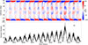 |
Fig. 1. Solar cycles obtained from the STABLE dynamo model. (a) Azimuthally averaged surface radial field as a function of latitude and time. (b) Temporal variation of the total (over the full-disk) monthly sunspot number. |
4. Results and discussion
We computed the monthly sunspot number and flux using the STABLE dynamo model to explore the underlying physical mechanisms and the spatiotemporal variations (QBOs and Rieger-type periods), as reported in various observational datasets (e.g., sunspot number, sunspot area, and subsurface flow fields) (Bazilevskaya et al. 2014; Inceoglu et al. 2021; Ravindra et al. 2022). Previous studies and observations suggest that the BMR tilt angle, magnetic flux of BMR, latitude distribution of BMR, and time delay between consecutive BMR emergence are the primary physical parameters that significantly influence the Babcock–Leighton mechanism (Karak & Miesch 2018; Cameron & Schüssler 2023; Kumar et al. 2024). These parameters also play a crucial role in the variability of the solar magnetic field and the asymmetry of the solar cycle (Baumann et al. 2004; Kumar et al. 2024). The STABLE model naturally incorporates all these physical parameters and produces cyclic magnetic fields. To investigate whether the Babcock–Leighton model produces short-term periodicities such as QBOs and Rieger-type periodicities, we employ Morlet wavelet power spectrum analysis along with the global wavelet power spectrum of both sunspot number and flux data. In our model, the BMR’s magnetic flux and sunspot number are intrinsically connected, leading to similar results in both sunspot number and flux analyses. Therefore, we present our results based on the sunspot number to maintain consistency with the observational data (e.g., sunspots and proxies of the solar magnetic field).
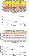 |
Fig. 2. Morlet and GWPS of monthly sunspot numbers obtained from the dynamo model with fluctuations in the BMR time delay. Panels (a–b): Short-term or Rieger-type periodicities. Panels (c–d): QBOs and other long-term periods including the main cycle period corresponding to the 11 year solar cycle. The dotted red lines in all GWPS represent the 95% confidence level and black dotted lines in Morlet wavelet spectra represent COI. |
To investigate the physical mechanism of QBOs and the Rieger-type periods, we first explore the role of individual fluctuating parameters (tilt scatter, flux variation, and time delay) that influence the Babcock–Leighton mechanism. We note that to study Rieger-type periodicities and QBOs in this model, we did not consider the case of the variation in the BMR latitude separately because it is not trivial to vary BMR latitude randomly by hand in this model. However, the mean latitude of the BMRs automatically varies with changes in the cycle strength in the model. In addition, we analyze the effect of the fluctuations in the combined parameters. Finally, in Subsection 4.2, we examine the effects of dynamo supercriticality on these periodicities. To do so, we gradually increased the value of Φ0 within a feasible range for the dynamo, keeping the rest of the parameters the same.
4.1. Effects of fluctuations in Babcock–Leighton process
In this subsection, we show the results of the individual Babcock–Leighton parameters and their combined impact on QBOs and Rieger periodicities. Note that we consider only the full-disk data to analyze the individual parameter’s effect on these periodicities, as the hemispheric data produce similar results as the full-disk data.
4.1.1. Time delay
First, we consider the effect of time delays in BMR emergence on QBOs and Rieger-type periodicities. To do so, in the STABLE model, we set a fixed value of the magnetic flux (1022 Mx), set the tilt fluctuations around Joy’s law to zero (σδ = 0), and computed the time delay from the distribution as given by Equation (5). We analyze the data using the Morlet wavelet analysis technique and GWPS (see Section 3). Figure 2(a) and (b) show the analysis of Rieger-type periods, and (c) and (d) for QBOs. The analysis of the simulated solar cycles reveals prominent periodicities at ∼12, 21, 47, 69, and 139 months (see Figure 2). The Morlet wavelet power spectrum and GWPS clearly indicate the presence of QBOs in the data, with a 95% confidence level. In Figure 2(a) and (c), the black dotted lines mark the COI in the Morlet wavelet analysis, and the thin black lines show periodicity contours above the 95% confidence level. In contrast, in Figure 2(b) and (d), the dotted red line denotes the 95% confidence boundary for the GWPS. The above analysis shows that only QBO signals are present in the data. This result suggests that the stochasticity in the time delay of BMR emergence can individually produce QBOs but not Rieger-type periods with the 95% significance level. This result is consistent with the findings of Wang & Sheeley (2003), who reported quasiperiodic variations with timescales of ∼1–3 years in the equatorial dipole moment and open flux derived from both SFT simulations and observed group sunspot areas. They suggested that the physical mechanism of these short-term periodicities is the stochastic fluctuations in the emergence rate of BMRs and their random longitudinal distribution on the solar surface.
4.1.2. Flux variation
Next, we examined the effect of flux variation on the QBOs and Rieger-type periodicity. For this, we did not fix the flux at 1022 Mx but computed it from the distribution given in Equation (7) so that the individual flux varied in a wide range consistent with observations. We fixed the time delay, and, as before, we did not include any scatter around Joy’s law. Applying Morlet wavelet analysis and GWPS to the sunspot flux time series obtained from this simulation, we find periodicities of ∼83 and 173 days, and 13, 37, 53, and 106 months (Figure A.1) in the Appendix. These periodicities differ from those obtained with time-delay variations. Here, we note that the data in this case exhibit clear signatures of Rieger periods and QBOs.
4.1.3. Tilt scatter around Joy’s law
In this case, we considered tilt scatter (σδ) of 15° around Joy’s law inspired by observations (Sreedevi et al. 2024) while keeping the magnetic flux and time delay fixed. The wavelet spectrum analysis of the data in this case reveals periodicities of ∼180 days, 16, 25, 33, 52, 73, and 147 months (see Figure A.2in the Appendix). This result also shows Rieger-type periodic signals and QBOs.
In all of the above cases, flux variation and tilt scatter-driven data show Rieger-type periods and QBOs. However, the time delay case does not show Rieger periods with a 95% significance level; it only shows QBOs. Moreover, the occurrence probability of Rieger-type periods is higher in the flux variation case, and the occurrence probability of QBOs is higher in the tilt-scatter case. Thus, this result suggests that in the Babcock–Leighton dynamo, for Rieger-type periodicity, fluctuation in the BMR flux plays a significant role, and for QBOs, tilt scatter plays a crucial role compared to the time delay. Next, we analyze the combined effect of all these fluctuations in the BMR parameters for the generation of QBOs and Rieger-type periodicities.
4.1.4. Combined fluctuations in Babcock–Leighton process
Now, we consider the fluctuations in all parameters of the Babcock–Leighton process, namely the tilt scatter around Joy’s law, variation in flux, latitude, and time delay. In contrast to the previous cases, here we analyze the hemispheric data in addition to the full-disk data. For the northern hemisphere, we find ∼82 and 170 days, 11, 38, and 142 month periodicities (Figure 3), while for the southern hemisphere, we find ∼83 and 173 days, 13, 39, 53, and 149 month periodicities (Figure A.3). Next, we analyze the periods for full-disk data, and we find ∼86 and 173 days, and 14, 39, 47, and 147 month periodicities in both the Morlet wavelet spectra and the GWPS (Figure A.4) with a 95% significance level.
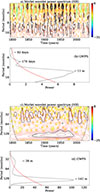 |
Fig. 3. Dynamical behavior of various periodicities observed in the northern hemisphere using wavelet power spectra for the monthly sunspot number time series data obtained from the model with fluctuations in all the parameters of the Babcock–Leighton process with a tilt scatter of σδ = 15°. Panel (a): Morlet wavelet spectra used to identify short-term periods (Rieger-type). Panel (b) Global power spectra for short-term periods (Rieger-type). The dotted red line represents a 95% confidence level. Panel (c): Similar to panel (a), but for the QBOs and long-range periods including the cycle corresponding to the 11 year solar cycle. Panel (d): Similar to panel (b), but for the study of QBOs and long periods. |
We recall that observational studies have reported Rieger-type periodicities in solar magnetic and proxy data, such as ∼60–85 days (Joshi et al. 2006), 154 days (Rieger et al. 1984), 160 days (Ballester et al. 2002), 155 days (Cho et al. 2014), 155–160 days (Zaqarashvili et al. 2010), 137–283 days (Ravindra et al. 2022), and 140–158 days (Chowdhury et al. 2024). Our model also reproduced similar Rieger-type periodicities in the range of ∼70–180 days (see Figures 3–A.4)(a and b). Furthermore, our model reproduced QBOs with periods ranging from ∼1 to 4.5 years (Figures 3–A.4)(c and d), which is in close agreement with the observed range of ∼1–4 years often found in various datasets (Bazilevskaya et al. 2014; Ravindra et al. 2022). We note that in our analysis, the Rieger-type periods and QBO contours with a 95% confidence level are not continuous and are confined primarily in the phase of solar maxima. Thus, the model results suggest that the Rieger-type periodicity and QBOs are intermittent, and that the occurrence probability is high during the solar maximum phase, consistent with observations (Ballester et al. 2002; Badalyan & Obridko 2011; Jain et al. 2023). Moreover, Gurgenashvili et al. (2017, 2021) studies show that Rieger-type periods and QBOs exhibit north-south asymmetry. Our model also reproduces different periodicities in Rieger-type periods and QBOs in both hemispheres (Table ). The reason for obtaining QBOs and Rieger-type periods in the Babcock–Leighton dynamo is the stochastic fluctuations and nonlinearity resulting from individual parameters (time delay, flux, latitude, and tilt) in the Babcock–Leighton process. Studies reveal that stochastic interactions in complex systems induce transient periodic or quasiperiodic behaviors (García-Ojalvo & Sancho 1996; Guo et al. 2017). Moreover, Olemskoy et al. (2013) suggest that the stochastic fluctuation in the Babcock–Leighton process with correlation times comparable to the solar rotation period can induce variability on shorter timescales.
Additionally, we observe the effect of tilt scatter around Joy’s law on Rieger-type periods and QBOs. We increased the tilt scatter (σδ) from 15° to 25° to see its effect on periodicities. We did not observe significant periodic variations in all cases, and the Rieger-type periodicity and QBOs were unaffected by the variation of tilt scatter. This behavior arises because, as the tilt scatter increases, the amplitude of polar field fluctuations becomes larger; thus, the strength of the next solar cycle increases. However, the cycle periodicity remains largely unaffected (Jiang et al. 2014b; Karak & Miesch 2017; Biswas et al. 2023). The periodicity of the solar cycle is primarily determined by the meridional flow, diffusivity, and α effect (Karak & Choudhuri 2011). Therefore, we did not observe any significant changes in QBOs and Rieger-type periods with the tilt scatter.
4.2. Effect of dynamo supercriticality
So far, our model operates at a weakly supercritical regime. Here, we want to explore the effect of dynamo supercriticality on the properties of QBOs and Rieger-type oscillations. To increase the supercriticality of the dynamo, we increased the value of Φ0 (i.e., boosted the BMR flux at higher values) from 2 to 4 and kept the other parameters fixed. We note that increasing the value of Φ0 made the generation of the polar field more efficient. Thus, this Φ0 parameter acts in a similar manner as the strength of α in 2D kinematic dynamo models and relates to the dynamo number (Miesch & Teweldebirhan 2016; Karak 2020). We find that when Φ0 is small, i.e., the dynamo is weakly supercritical, we find periodicities of ∼86 and 173 days, 39, 47, and 147 months in full-disk data, which correspond to Rieger-type periodicity and QBOs, as observed in various observational data (Bazilevskaya et al. 2014). However, as the dynamo supercriticality increases, the occurrence probability of Rieger-type periodicity decreases. When the values of Φ0 are considerably high, the dynamo operates in a highly supercritical regime, and we find only QBO-like periodicities with a 95% significance level (see Figure 4). The reason is that, as the supercriticality of the dynamo increases, the effect of fluctuations on the magnetic field is suppressed due to the increasing influence of nonlinearity (Kumar et al. 2021b or see, Fig. 16 of Karak 2023). As a result, the Babcock–Leighton dynamo in the supercritical regime fails to produce Rieger-type short-term periods (see Figure 4(a) and (b) and Table ). However, in this regime, the dynamo still produces QBO features (Figure 4(c) and (d)).
Short-term (Rieger-type) periods, QBOs, and regular cycle corresponding to 11 year solar cycle at varying dynamo supercriticality as measured by Φ0.
Next, our analysis shows ∼41 and 80 month periods in a highly supercritical dynamo, as shown in Figure 4(c) and (d). Here, we note that the 80 month periodicity corresponds to the dominant or regular period (11 years for the Sun), which is reduced from 12.25 years at Φ0 = 2. This reduction in the length of the regular cycle is due to the operation of the dynamo at a highly supercritical regime. It was already known that increasing the dynamo supercriticality decreases the cycle duration due to the efficient generation of the poloidal field (Noyes et al. 1984); see Table 2 of Kumar et al. (2021b). Furthermore, in our dynamo simulations, we observe that with increasing dynamo supercriticality, the regular or dominant cycle period decreases at a faster rate than the other short-term periodicities (Table ). The reason is that the fundamental periods of the solar cycle are primarily governed by the combined effect of the efficiency of poloidal field generation (Φ0 in the present case) and large-scale flows (Dikpati & Charbonneau 1999; Karak 2010), which remain unchanged here. With the increase of Φ0, the polar field buildup rate increases; thus, polarity reversal occurs earlier than usual (Charbonneau 2020; Golubeva et al. 2023). This results in a decrease in the periods of the regular cycle. However, the short-term periods are determined by the coherence time of stochastic fluctuations, which remains constant in our model. Thus, the QBOs and Rieger-type periodicities remain almost unaffected. We note a slight decrease because of the increase in the dynamo efficiency.
5. Conclusions
In this study, we explore QBO and Rieger-type periods and their physical mechanisms in the Babcock–Leighton dynamo. For this, we used a 3D Babcock–Leighton dynamo model (STABLE), which captures the realistic properties of the BMRs and closely connects the model with observed solar magnetic features. For the first time, we show that the Babcock–Leighton dynamo can produce Rieger-type periods and QBOs as seen in different observational data (Rieger et al. 1984; Bazilevskaya et al. 2014). In particular, we investigated the role of individual Babcock–Leighton parameters relating to BMR properties for Rieger-type periodicity and QBOs. We find that fluctuations in all individual Babcock–Leighton parameters, namely the distributions of the BMR time delay, flux, tilt angle, and latitude can successfully reproduce the QBOs of periodicities between ∼1 to 4.5 years and Rieger-type periods with a 95% significance level except for the case of time delay fluctuations, for which we observed only QBOs. Moreover, when the fluctuations in all the parameters of the Babcock–Leighton process act together, the probability of occurrence of QBOs and Rieger periods increases significantly due to the interaction of different stochastic fluctuations in the Babcock–Leighton process (Pipin et al. 2012; Schüssler & Cameron 2018; Cameron & Schüssler 2019). Next, we analyzed the sensitivity of the tilt scatter on the QBOs and Rieger periodicities. We find that the varying tilt scatter does not significantly affect the QBOs and Rieger-type periodicity and appearance.
We note that Inceoglu et al. (2019) could not find Rieger-type periods or QBOs in their 2D Babcock–Leighton dynamo model. A possible explanation could be that the Babcock–Leighton process is inherently 3D, and in the 2D model, this is represented by a single term α, which may not adequately capture all the complex fluctuating properties of the BMR required to reproduce such mid-term periodicities.
Finally, we investigate the effect of dynamo supercriticality on these periodicities. We find that when the dynamo operates near the critical region, the Babcock–Leighton dynamo reproduces Rieger-type periodicities and QBOs successfully. However, as we increase the supercriticality of the dynamo, the probability of occurrence of Rieger-type periodicity decreases, and in a highly supercritical regime, the dynamo fails to reproduce the Rieger-type periods, while QBOs are still produced with a 95% significance level. This result presents independent evidence for the suggestion that the solar dynamo is not highly supercritical (e.g., Vashishth et al. 2023; Ghosh et al. 2024; Wavhal et al. 2025). Furthermore, we find a decrease in the periodicity of the Rieger-type, QBOs, and regular cycle with the dynamo supercriticality. This result supports the observational findings that weaker cycles show longer Rieger-type periodicities (∼185–195 days), whereas stronger cycles have shorter ones (∼155–165 days) (Gurgenashvili et al. 2017). In conclusion, our 3D Babcock–Leighton dynamo model including stochastic fluctuations in the BMR parameters successfully reproduces QBOs and Rieger-type periodicities along with their intermittent and asymmetric properties–the key observational features of the solar cycle.
Acknowledgments
The authors thank the anonymous referee for offering constructive comments that helped to improve the quality of the manuscript to a large extent. The authors also acknowledge the computational support and the resources provided by the IIA computing facility. B.B.K. acknowledges the financial support from the Indian Space Research Organization (project no. ISRO/RES/RAC-S/IITBHU/2024-25).
References
- Babcock, H. W. 1961, ApJ, 133, 572 [Google Scholar]
- Badalyan, O. G., & Obridko, V. N. 2011, New Astron., 16, 357 [NASA ADS] [CrossRef] [Google Scholar]
- Ballester, J. L., Oliver, R., & Carbonell, M. 2002, ApJ, 566, 505 [NASA ADS] [CrossRef] [Google Scholar]
- Baumann, I., Schmitt, D., Schüssler, M., & Solanki, S. K. 2004, A&A, 426, 1075 [NASA ADS] [CrossRef] [EDP Sciences] [Google Scholar]
- Bazilevskaya, G. A., Krainev, M. B., Makhmutov, V. S., et al. 2000, Sol. Phys., 197, 157 [Google Scholar]
- Bazilevskaya, G., Broomhall, A.-M., Elsworth, Y., & Nakariakov, V. M. 2014, Space Sci. Rev., 186, 359 [CrossRef] [Google Scholar]
- Benevolenskaya, E. E. 1998, ApJ, 509, L49 [Google Scholar]
- Biswas, A., Karak, B. B., & Kumar, P. 2023, MNRAS, 526, 3994 [Google Scholar]
- Cameron, R. H., & Schüssler, M. 2012, A&A, 548, A57 [NASA ADS] [CrossRef] [EDP Sciences] [Google Scholar]
- Cameron, R. H., & Schüssler, M. 2019, A&A, 625, A28 [NASA ADS] [CrossRef] [EDP Sciences] [Google Scholar]
- Cameron, R. H., & Schüssler, M. 2023, Space Sci. Rev., 219, 60 [NASA ADS] [CrossRef] [Google Scholar]
- Charbonneau, P. 2020, Liv. Rev. Sol. Phys., 17, 4 [Google Scholar]
- Cho, I.-H., Hwang, J., & Park, Y.-D. 2014, Sol. Phys., 289, 707 [Google Scholar]
- Chowdhury, P., Khan, M., & Ray, P. C. 2009, MNRAS, 392, 1159 [Google Scholar]
- Chowdhury, P., Jain, R., & Awasthi, A. K. 2013, ApJ, 778, 28 [Google Scholar]
- Chowdhury, P., Belur, R., Bertello, L., & Pevtsov, A. A. 2022, ApJ, 925, 81 [NASA ADS] [CrossRef] [Google Scholar]
- Chowdhury, P., Kilcik, A., Saha, A., et al. 2024, Sol. Phys., 299, 19 [Google Scholar]
- Dasi-Espuig, M., Solanki, S. K., Krivova, N. A., Cameron, R., & Peñuela, T. 2010, A&A, 518, A7 [NASA ADS] [CrossRef] [EDP Sciences] [Google Scholar]
- Dey, B., Sreedevi, A., & Karak, B. B. 2025, ApJ, 993, 196 [Google Scholar]
- Dikpati, M., & Charbonneau, P. 1999, ApJ, 518, 508 [NASA ADS] [CrossRef] [Google Scholar]
- Dikpati, M., Cally, P. S., McIntosh, S. W., & Heifetz, E. 2017, Sci. Rep., 7, 14750 [NASA ADS] [CrossRef] [Google Scholar]
- Dikpati, M., McIntosh, S. W., Bothun, G., et al. 2018, ApJ, 853, 144 [Google Scholar]
- Dikpati, M., McIntosh, S. W., & Wing, S. 2021, Front. Astron. Space Sci., 8, 71 [Google Scholar]
- Eddy, J. A. 1976, Science, 192, 1189 [NASA ADS] [CrossRef] [Google Scholar]
- Edmonds, I. R. 2016, Sol. Phys., 291, 203 [Google Scholar]
- García-Ojalvo, J., & Sancho, J. M. 1996, Phys. Rev. E, 53, 5680 [Google Scholar]
- Ghosh, A., Kumar, P., Prasad, A., & Karak, B. B. 2024, AJ, 167, 209 [Google Scholar]
- Gizon, L., Cameron, R. H., Pourabdian, M., et al. 2020, Science, 368, 1469 [Google Scholar]
- Gleissberg, W. 1939, Observatory, 62, 158 [Google Scholar]
- Gnevyshev, M. N. 1977, Sol. Phys., 51, 175 [NASA ADS] [CrossRef] [Google Scholar]
- Golubeva, E. M., Biswas, A., Khlystova, A. I., Kumar, P., & Karak, B. B. 2023, MNRAS, 525, 1758 [Google Scholar]
- Guo, K., Jiang, J., & Xu, Y. 2017, Entropy, 19, 280 [Google Scholar]
- Gurgenashvili, E., Zaqarashvili, T. V., Kukhianidze, V., et al. 2017, ApJ, 845, 137 [NASA ADS] [CrossRef] [Google Scholar]
- Gurgenashvili, E., Zaqarashvili, T. V., Kukhianidze, V., et al. 2021, A&A, 653, A146 [NASA ADS] [CrossRef] [EDP Sciences] [Google Scholar]
- Hathaway, D. H., Wilson, R. M., & Reichmann, E. J. 2002, Sol. Phys., 211, 357 [Google Scholar]
- Hazra, G., & Choudhuri, A. R. 2019, ApJ, 880, 113 [Google Scholar]
- Howe, R., Christensen-Dalsgaard, J., Hill, F., et al. 2000, Science, 287, 2456 [Google Scholar]
- Inceoglu, F., Simoniello, R., Arlt, R., & Rempel, M. 2019, A&A, 625, A117 [NASA ADS] [CrossRef] [EDP Sciences] [Google Scholar]
- Inceoglu, F., Howe, R., & Loto’aniu, P. T. M. 2021, ApJ, 920, 49 [NASA ADS] [CrossRef] [Google Scholar]
- Jain, K., Chowdhury, P., & Tripathy, S. C. 2023, ApJ, 959, 16 [NASA ADS] [CrossRef] [Google Scholar]
- Jha, B. K., Karak, B. B., Mandal, S., & Banerjee, D. 2020, ApJ, 889, L19 [NASA ADS] [CrossRef] [Google Scholar]
- Jiang, J. 2020, ApJ, 900, 19 [Google Scholar]
- Jiang, J., Cameron, R. H., & Schüssler, M. 2014a, ApJ, 791, 5 [Google Scholar]
- Jiang, J., Hathaway, D. H., Cameron, R. H., et al. 2014b, Space Sci. Rev., 186, 491 [Google Scholar]
- Jiang, J., Wang, J.-X., Jiao, Q.-R., & Cao, J.-B. 2018, ApJ, 863, 159 [NASA ADS] [CrossRef] [Google Scholar]
- Joshi, B., Pant, P., & Manoharan, P. K. 2006, A&A, 452, 647 [NASA ADS] [CrossRef] [EDP Sciences] [Google Scholar]
- Jouve, L., Proctor, M. R. E., & Lesur, G. 2010, A&A, 519, A68 [CrossRef] [EDP Sciences] [Google Scholar]
- Käpylä, M. J., Käpylä, P. J., Olspert, N., et al. 2016, A&A, 589, A56 [NASA ADS] [CrossRef] [EDP Sciences] [Google Scholar]
- Karak, B. B. 2010, ApJ, 724, 1021 [CrossRef] [Google Scholar]
- Karak, B. B. 2020, ApJ, 901, L35 [NASA ADS] [CrossRef] [Google Scholar]
- Karak, B. B. 2023, Liv. Rev. Sol. Phys., 20, 3 [NASA ADS] [CrossRef] [Google Scholar]
- Karak, B. B., & Cameron, R. 2016, ApJ, 832, 94 [NASA ADS] [CrossRef] [Google Scholar]
- Karak, B. B., & Choudhuri, A. R. 2011, MNRAS, 410, 1503 [NASA ADS] [Google Scholar]
- Karak, B. B., & Miesch, M. 2017, ApJ, 847, 69 [NASA ADS] [CrossRef] [Google Scholar]
- Karak, B. B., & Miesch, M. 2018, ApJ, 860, L26 [NASA ADS] [CrossRef] [Google Scholar]
- Karak, B. B., Jiang, J., Miesch, M. S., Charbonneau, P., & Choudhuri, A. R. 2014, Space Sci. Rev., 186, 561 [CrossRef] [Google Scholar]
- Karak, B. B., Käpylä, P. J., Käpylä, M. J., et al. 2015, A&A, 576, A26 [NASA ADS] [CrossRef] [EDP Sciences] [Google Scholar]
- Karak, B. B., Mandal, S., & Banerjee, D. 2018, ApJ, 866, 17 [CrossRef] [Google Scholar]
- Kitchatinov, L. L., & Olemskoy, S. V. 2011, Astron. Lett., 37, 656 [NASA ADS] [CrossRef] [Google Scholar]
- Knaack, R., & Stenflo, J. O. 2005, A&A, 438, 349 [NASA ADS] [CrossRef] [EDP Sciences] [Google Scholar]
- Korsós, M. B., Dikpati, M., Erdélyi, R., Liu, J., & Zuccarello, F. 2023, ApJ, 944, 180 [CrossRef] [Google Scholar]
- Kumar, P., Nagy, M., Lemerle, A., Karak, B. B., & Petrovay, K. 2021a, ApJ, 909, 87 [NASA ADS] [CrossRef] [Google Scholar]
- Kumar, P., Karak, B. B., & Vashishth, V. 2021b, ApJ, 913, 65 [Google Scholar]
- Kumar, P., Biswas, A., & Karak, B. B. 2022, MNRAS, 513, L112 [Google Scholar]
- Kumar, P., Karak, B. B., & Sreedevi, A. 2024, MNRAS [arXiv:2404.10526] [Google Scholar]
- Leighton, R. B. 1969, ApJ, 156, 1 [Google Scholar]
- Mandal, S., Karak, B. B., & Banerjee, D. 2017, ApJ, 851, 70 [Google Scholar]
- McIntosh, S. W., Leamon, R. J., Krista, L. D., et al. 2015, Nat. Commun., 6, 6491 [NASA ADS] [CrossRef] [Google Scholar]
- Miesch, M. S., & Dikpati, M. 2014, ApJ, 785, L8 [NASA ADS] [CrossRef] [Google Scholar]
- Miesch, M. S., & Teweldebirhan, K. 2016, Adv. Space Res., 58, 1571 [NASA ADS] [CrossRef] [Google Scholar]
- Mordvinov, A. V., Karak, B. B., Banerjee, D., et al. 2022, MNRAS, 510, 1331 [Google Scholar]
- Morlet, J., Arens, G., Forgeau, I., & Giard, D. 1982, Geophysics, 47, 203 [NASA ADS] [CrossRef] [Google Scholar]
- Muñoz-Jaramillo, A., Senkpeil, R. R., Windmueller, J. C., et al. 2015, ApJ, 800, 48 [Google Scholar]
- Noyes, R. W., Weiss, N. O., & Vaughan, A. H. 1984, ApJ, 287, 769 [Google Scholar]
- Olemskoy, S. V., Choudhuri, A. R., & Kitchatinov, L. L. 2013, Astron. Rep., 57, 458 [Google Scholar]
- Parker, E. N. 1955, ApJ, 122, 293 [Google Scholar]
- Petrovay, K. 2020, Liv. Rev. Sol. Phys., 17, 2 [Google Scholar]
- Pipin, V. V., Sokoloff, D. D., & Usoskin, I. G. 2012, A&A, 542, A26 [NASA ADS] [CrossRef] [EDP Sciences] [Google Scholar]
- Qin, L., Jiang, J., & Wang, R. 2025, ApJ, 986, 114 [Google Scholar]
- Rajaguru, S. P., & Antia, H. M. 2015, ApJ, 813, 114 [Google Scholar]
- Ravindra, B., Chowdhury, P., Ray, P. C., & Pichamani, K. 2022, ApJ, 940, 43 [Google Scholar]
- Rieger, E., Share, G. H., Forrest, D. J., et al. 1984, Nature, 312, 623 [Google Scholar]
- Ruzmaikin, A., Cadavid, A.C., & Lawrence, J. 2008, JASTP, 70, 2112 [Google Scholar]
- Schou, J., Antia, H. M., Basu, S., et al. 1998, ApJ, 505, 390 [Google Scholar]
- Schüssler, M., & Cameron, R. H. 2018, A&A, 618, A89 [NASA ADS] [CrossRef] [EDP Sciences] [Google Scholar]
- Simoniello, R., Jain, K., Tripathy, S. C., et al. 2013, ApJ, 765, 100 [Google Scholar]
- Solanki, S. K., Wenzler, T., & Schmitt, D. 2008, A&A, 483, 623 [NASA ADS] [CrossRef] [EDP Sciences] [Google Scholar]
- Sreedevi, A., Jha, B. K., Karak, B. B., & Banerjee, D. 2024, ApJ, 966, 112 [Google Scholar]
- Steenbeck, M., Krause, F., & Rädler, K. H. 1966, Z. Naturforsch. A, 21, 369 [Google Scholar]
- Stenflo, J. O., & Kosovichev, A. G. 2012, ApJ, 745, 129 [NASA ADS] [CrossRef] [Google Scholar]
- Strugarek, A., Beaudoin, P., Charbonneau, P., & Brun, A. S. 2018, ApJ, 863, 35 [Google Scholar]
- Suess, H. E. 1980, Radiocarbon, 22, 200 [NASA ADS] [CrossRef] [Google Scholar]
- Torrence, C., & Compo, G. P. 1998, BAMS, 79, 61 [NASA ADS] [CrossRef] [Google Scholar]
- Usoskin, I. G. 2023, Liv. Rev. Sol. Phys., 20, 2 [NASA ADS] [CrossRef] [Google Scholar]
- Vashishth, V., Karak, B. B., & Kitchatinov, L. 2023, MNRAS, 522, 2601 [NASA ADS] [CrossRef] [Google Scholar]
- Vecchio, A., & Carbone, V. 2009, A&A, 502, 981 [NASA ADS] [CrossRef] [EDP Sciences] [Google Scholar]
- Wang, Y. M., & Sheeley, N. R., Jr 2003, ApJ, 590, 1111 [Google Scholar]
- Wang, Y. M., Colaninno, R. C., Baranyi, T., & Li, J. 2015, ApJ, 798, 50 [Google Scholar]
- Wavhal, S., Kumar, P., & Karak, B. B. 2025, Sol. Phys., 300, 21 [Google Scholar]
- Zaqarashvili, T. V., Carbonell, M., Oliver, R., & Ballester, J. L. 2010, ApJ, 709, 749 [NASA ADS] [CrossRef] [Google Scholar]
Appendix A: Supporting figures
Here, Figure A.1 and Figure A.2 respectively show the effects of stochastic fluctuations in flux and tilt on the QBOs and Rieger-type periodicities. These figures are similar to Figure 2 of the time delay case. Additionally, Figure A.3 and Figure A.4 depict the effects of combined stochastic fluctuations in the Babcock–Leighton process on the QBOs and Rieger-type periodicities in the southern hemisphere and full-disk solar data, respectively. These figures are also similar to Figure 3.
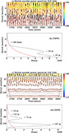 |
Fig. A.2. Same as Figure 2, but with tilt fluctuations around Joy’s law only with σδ = 15° and a fixed time delay and flux. |
All Tables
Short-term (Rieger-type) periods, QBOs, and regular cycle corresponding to 11 year solar cycle at varying dynamo supercriticality as measured by Φ0.
All Figures
|
Fig. 1. Solar cycles obtained from the STABLE dynamo model. (a) Azimuthally averaged surface radial field as a function of latitude and time. (b) Temporal variation of the total (over the full-disk) monthly sunspot number. |
| In the text | |
|
Fig. 2. Morlet and GWPS of monthly sunspot numbers obtained from the dynamo model with fluctuations in the BMR time delay. Panels (a–b): Short-term or Rieger-type periodicities. Panels (c–d): QBOs and other long-term periods including the main cycle period corresponding to the 11 year solar cycle. The dotted red lines in all GWPS represent the 95% confidence level and black dotted lines in Morlet wavelet spectra represent COI. |
| In the text | |
|
Fig. 3. Dynamical behavior of various periodicities observed in the northern hemisphere using wavelet power spectra for the monthly sunspot number time series data obtained from the model with fluctuations in all the parameters of the Babcock–Leighton process with a tilt scatter of σδ = 15°. Panel (a): Morlet wavelet spectra used to identify short-term periods (Rieger-type). Panel (b) Global power spectra for short-term periods (Rieger-type). The dotted red line represents a 95% confidence level. Panel (c): Similar to panel (a), but for the QBOs and long-range periods including the cycle corresponding to the 11 year solar cycle. Panel (d): Similar to panel (b), but for the study of QBOs and long periods. |
| In the text | |
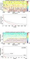 |
Fig. 4. Same as Figure 3, but at a highly supercritical regime of the dynamo with Φ0 = 4. |
| In the text | |
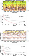 |
Fig. A.1. Same as Figure 2, but for flux fluctuations only. |
| In the text | |
|
Fig. A.2. Same as Figure 2, but with tilt fluctuations around Joy’s law only with σδ = 15° and a fixed time delay and flux. |
| In the text | |
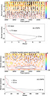 |
Fig. A.3. Similar to Figure 3, but for the southern hemisphere. |
| In the text | |
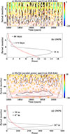 |
Fig. A.4. Similar to Figure 3, but for the full-disk data. |
| In the text | |
Current usage metrics show cumulative count of Article Views (full-text article views including HTML views, PDF and ePub downloads, according to the available data) and Abstracts Views on Vision4Press platform.
Data correspond to usage on the plateform after 2015. The current usage metrics is available 48-96 hours after online publication and is updated daily on week days.
Initial download of the metrics may take a while.