| Issue |
A&A
Volume 705, January 2026
|
|
|---|---|---|
| Article Number | A145 | |
| Number of page(s) | 12 | |
| Section | The Sun and the Heliosphere | |
| DOI | https://doi.org/10.1051/0004-6361/202556300 | |
| Published online | 15 January 2026 | |
Modelling the total solar eclipse in 2024 with COCONUT
1
Department of Mathematics/Centre for mathematical Plasma Astrophysics, KU Leuven Celestijnenlaan 200B 3001 Leuven, Belgium
2
Institute of Physics, University of Maria Curie-Skłodowska ul. Radziszewskiego 10 20-031 Lublin, Poland
★ Corresponding author: This email address is being protected from spambots. You need JavaScript enabled to view it.
Received:
8
July
2025
Accepted:
30
October
2025
Abstract
Context. Coronal modelling is crucial for a better understanding of solar physics and heliophysics. Accurate plasma conditions at the outer boundary of a solar corona lead to more precise space weather predictions. Because the Sun is so very bright and we lack white-light (WL) observations of the solar atmosphere and low corona (1–1.5 R⊙), total solar eclipses have become a standard approach for validating the coronal models. We validate the coronal model COCONUT by predicting the coronal configuration during the total solar eclipse on April 8, 2024.
Aims. We aim to predict the accurate configuration of the solar corona during the total solar eclipse on April 8, 2024. Additionally, we compare the predictive capabilities in the steady and dynamic driving of the boundary conditions in COCONUT. We used a full 3D magnetohydrodynamics (MHD) model to reconstruct the solar corona from the solar surface to 30 R⊙.
Methods. We started by predicting the upcoming total solar eclipse on March 21. The predictions were conducted in three different regimes: quasi-steady driving of the inner boundary conditions (BCs) with a daily cadence, and dynamic driving of the inner BCs with daily and hourly cadences. The results from all the simulations were compared to the total solar eclipse images. Additionally, the synthetic WL images were generated from the Solar Terrestrial Relations Observatory Ahead (STEREO-A) field of view and compared to COR2 observed images. The normalised polarised brightness was compared in the COR2 and synthetic WL images.
Results. The predicted solar corona does not vary significantly in the first half of the prediction window because the observations of the magnetic field are not yet accurately updated on the solar surface corresponding to April 8. The magnetic field changes more significantly as the eclipse date approaches. The dynamic simulations yielded better results than the quasi-steady predictions. Driving the simulations at a higher cadence did not significantly improve the results because the magnetic field maps are highly processed. The west limb was better reconstructed in the simulations than the east limb.
Conclusions. We predicted the total solar eclipse coronal configuration 18 days before the total solar eclipse. We conclude that the dynamic simulations produced more accurate predictions. The availability of comprehensive observations is crucial because the emergence of the active region on the east limb made it difficult to accurately predict the east-limb coronal configuration because the input of the magnetic field data was incorrect. More detailed input BCs are necessary for reconstructing smaller-scale structures in the corona.
Key words: magnetohydrodynamics (MHD) / methods: numerical / methods: observational / Sun: corona / Sun: magnetic fields
© The Authors 2026
 Open Access article, published by EDP Sciences, under the terms of the Creative Commons Attribution License (https://creativecommons.org/licenses/by/4.0), which permits unrestricted use, distribution, and reproduction in any medium, provided the original work is properly cited.
This article is published in open access under the Subscribe to Open model. This email address is being protected from spambots. You need JavaScript enabled to view it. to support open access publication.
1. Introduction
Complex physical processes take place in the solar corona. These processes are not fully understood because it is difficult or even impossible to observe them. This creates a significant lack of available data for testing different theories and validating models. The solar corona is faint compared to the luminosity from the solar surface. Therefore, it is impossible to distinguish the details that characterise different phenomena in the solar corona. The standard approach has become to test various theories about the processes in the solar atmosphere with coronal modelling. It is crucial to validate the modelled corona to advance our knowledge and understanding of solar physics. Because we lack white-light coronagraph observations in the low solar corona 1–1.5 R⊙, total solar eclipses have become a standard way of assessing the performance of coronal models. Total solar eclipses constrain the validation period of coronal modelling because they occur infrequently. This currently is the only way of distinguishing the features in the low corona close to the solar surface, however. Total solar eclipses represent a single snapshot of the solar coronal configuration in time, while for time-dependent simulations, continuous white-light observations are necessary. In the near future, the PROBA-3 mission will provide us with continuous white-light (WL) images of the corona, starting from near the solar surface (Zhukov et al. 2025). Pictures taken during total solar eclipses remain one of the most popular ways of validating coronal models to date.
A total solar eclipse occurred on April 8, 2024, during the maximum of solar cycle 25. Therefore, the eclipse images revealed a very complex structure of the solar corona, with multiple streamers and a prominence that was visible on the south-west limb of the Sun. The total solar eclipse of 2024 presents an excellent opportunity to test the performance of coronal models, but it is also very challenging because of the strong magnetic fields and gradients that occur during solar maximum.
Numerous global coronal models have been developed over the years. One of the oldest and most mature numerical models is magnetohydrodynamics (MHD) around a sphere (MAS) by Predictive Science Inc. (Mikić et al. 1999; Mikic & Linker 1996). The team has advanced the model, starting from the total solar eclipse in 1996, and has shown increasingly accurate predictions since the late 1990s. Downs et al. (2025) reported the results of modelling the same eclipse event performed by the MAS model. Another advanced global MHD model is the AWSoM model (van der Holst et al. 2014), which uses the Alfvén wave heating mechanism for the solar wind acceleration. Other models, such as MULTI-VP (Pinto & Rouillard 2017), SIP-IFVM (Wang et al. 2025c), Wind-Predict (Réville et al. 2016, 2020), and a 3D MHD model developed by Usmanov et al. (2014, 2018), also focused on global coronal structures using various approaches. Numerical computations in the coronal domain are relatively expensive and complex. The outcome strongly depends on the imposed boundary conditions and on the implemented physics and numerical techniques.
Recently, a new, optimised 3D global coronal modelling tool called coolfluid corona unstructured (COCONUT) (Perri et al. 2022) was developed within the framework of the platformComputational Object-Oriented Libraries for Fluid Dynamics (Lani et al. 2005; Kimpe et al. 2005; Lani et al. 2006, 2013, 2014, COOLFluiD). The first version of COCONUT was polytropic and primarily focused on the inner corona structures near the Sun. Later, Baratashvili et al. (2024) upgraded the polytropic COCONUT model to a full MHD model, including source and sink terms in the equations to accelerate and decelerate the solar wind to obtain a bi-modal distribution of the solar wind velocity. This upgraded COCONUT model is suitable for space weather purposes because the output of the corona model was successfully coupled to the heliospheric models Icarus (Baratashvili et al. 2025) and EUHFORIA (Pomoell & Poedts 2018). This upgraded version of COCONUT is constrained by static magnetograms that are used as inner boundary conditions for the radial magnetic field component. Moreover, Wang et al. (2025a) and Wang et al. (2025b) extended COCONUT to a more realistic, time-evolving coronal model driven by a series of subsequent magnetograms that are interpolated to generate time-dependent boundary conditions.
This paper uses the 2024 total solar eclipse to validate the novel global 3D MHD coronal model COCONUT. The predictions began on March 21, 2024, in a quasi-steady state regime and were updated daily with the latest magnetogram data from the GONG observatory. After the total solar eclipse, we used the observed photospheric magnetic field closest to the eclipse time to drive the coronal model. Additionally, we performed the simulations in the time-dependent regime, with daily and hourly updated magnetic field information at the inner boundary. Section 2 describes the numerical setup in COCONUT and section 3 focuses on the input data for various simulations. The predicted solar corona and multiple validation techniques are described in section 4 for all the simulation setups. Finally, we present our conclusions in section 5.
2. Numerical setup in COCONUT
COCONUT is a 3D MHD coronal model with a domain starting from near the solar surface to 30 R⊙. The data-driven model uses the observed photospheric magnetic field to model its corona. We solved the 3D MHD equations in their conservative form, which reads
 (1)
(1)
where E denotes the total energy  , B is the magnetic field, V is the velocity field, g is the gravitational acceleration, ρ is the plasma density, and p is the thermal pressure. The gravitational acceleration is given by
  and the identity dyadic
  . The closure is given by the ideal equation of state which for the internal energy density is
  , with an adiabatic index γ of 5/3. The solar rotation was considered by prescribing the Vϕ component at the inner boundary (Kuźma et al. 2023). S represents the source and sink terms, including thermal conductivity, radiative losses, and an ad hoc coronal heating function on the right-hand side of the energy equation, S = −∇⋅q + Qrad + QH. The source and sink terms were described in detail by Baratashvili et al. (2024). For the approximated heating function, we chose the following formulation:
 (2)
(2)
where H0 = 4 ⋅ 10−5 erg cm−3 s−1 G−1 and λ = 0.7 R⊙.
The last equation was introduced to ensure the divergence-free constraint ∇ ⋅ B = 0 and ϕ is a scalar potential function that constrains B to the space of divergence-free fields. We used the artificial compressibility analogy (Chorin 1997), which is similar to hyperbolic divergence cleaning (Dedner et al. 2002) and performs well with implicit solvers Yalim et al. (2011). Vref denotes the propagation speed of the numerical divergence error. In this way, the whole equation system remained hyperbolic.
Solar activity during the 2024 solar eclipse was high, and we therefore used a low-resolution mesh to avoid extreme gradients in the computational domain. We used an unstructured fifth-level subdivided geodesic polyhedron mesh starting from 1 R⊙ to 30 R⊙. The computational domain comprised approximately 380 000 finite-volume elements. A detailed description of the mesh was given by Brchnelova et al. (2022b). We imposed uniform initial boundary conditions for the plasma variables. The computational domain here started above the transition region, and we used the characteristic parameter values for the base of the solar corona. We chose the commonly prescribed values for the density and temperature characteristic for the base of the solar corona, namely n⊙ = 2 × 108 cm−3 and T = 1.8 × 10⁶ K. We used the magnetic field derived from the magnetogram in a smoothing procedure to determine the inner boundary conditions for the radial magnetic field component. More details about the processing of the magnetogram are given in section 3. We used a Dirichlet boundary condition for the Br magnetic field component. The procedure for the magnetic field driving was similar to the procedure described in Kuźma et al. (2023) and Baratashvili et al. (2024). The magnetic field components in the other spatial directions (Bθ and Bϕ) were allowed to evolve freely and were defined as the corresponding values at the centroid of the nearest inner cell. The velocity was set so the plasma flows along the magnetic field lines (Brchnelova et al. 2022a).
3. Simulation setup
The predictions for the total solar eclipse on April 8, 2024, started on March 21, 2024. We chose the magnetogram product from the GONG (Global Oscillation Network Group) observatory. As reported by Perri et al. (2022), Kuźma et al. (2023) and Baratashvili et al. (2024), a spherical harmonic decomposition was used to pre-process the maps. Due to the high solar activity, the spherical harmonics beyond ℓmax = 10 were filtered out. Thus, the obtained maps were heavily smoothed. Initially, the predictions were made with steady simulations with a 24-hour cadence at 19:00 UT daily. This led to quasi-dynamic predictions of the total solar eclipse evolving over 18 days leading up to the eclipse day. We selected four points in time and corresponding snapshots from the entire prediction window to minimise excessive data and overwhelming information.
Figure 1 shows the original and processed magnetograms. The upper left magnetogram corresponds to the start of the prediction window on March 21. For better comparison, the original and processed magnetograms were saturated to the [−20, 20] G range for all shown magnetograms. The upper right panel corresponds to the solar magnetic field configuration after one week. The rectangles indicate the regions where the most prominent difference between the plotted magnetograms was observed. These regions were identified by considering at the structure of the magnetic field in the input map and the difference between the maps given in Figure A.1. The rectangle labelled ‘1’ is plotted in both magnetograms to show and emphasise that the magnetic field within this area changed significantly in this period. The difference is especially noticeable to the naked eye in the lower part of the rectangle. The lower left panel corresponds to April 3. Here, a more substantial change is visible in the area enclosed in rectangle 2 compared to the configuration of the solar magnetic field on March 28. The lower right panel corresponds to the day of the total solar eclipse. The two regions enclosed by boxes 2 and 3 are significantly different from the magnetic field observed on April 3. These areas significantly affect the coronal configuration from the Earth’s point of view, which results in variable predictions as the eclipse day approaches.
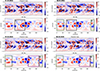 |
Fig. 1. Original GONG (upper panels) and pre-processed input magnetograms (lower panels) for March 21, March 28, April 3 and April 8. The colour maps are saturated to the [−20, 20] G range. All maps are rotated so that they are aligned with the Earth’s view angle as of April 8, 2024. Squares 1, 2 and 3 represent the areas of interest. |
For the dynamic (time-dependent) regime, which is necessary to capture the continuous temporal evolution of the coronal structures, we set the time step to 5 minutes to balance computational efficiency with the desired numerical stability and accuracy (Wang et al. 2025a,c). We drove the coronal evolution using a series of hourly updated and another series of daily updated magnetograms. We applied a cubic Hermite interpolation to derive the inner boundary magnetic field at each physical time step (Wang et al. 2025a,c). For comparison with the quasi-steady predictions, the simulations with the time-evolving COCONUT version were performed with daily updated magnetograms and later with hourly updated magnetograms. In both cases, magnetograms at each physical time step were interpolated from the temporally nearest observed magnetograms. Thus, simulations in the quasi-steady and dynamic regimes were driven by the same magnetograms, with different cadences and driving modes.
4. Predictions of the total solar eclipse
The predictions of the total solar eclipse were made in the quasi-steady and dynamic regimes. The effect of updating the inner boundary conditions was also investigated. We wished to assess which approach yielded more accurate predictions. Since the input magnetic field was smoothened and a low-resolution computational grid was used, we used various techniques to validate the modelled corona and present the most comprehensive assessment of its strengths and weaknesses. Below, all different regimes are considered separately, first with the coronal validation method reported by Wagner et al. (2022) section 3.2.1 in the cited paper. The model focuses on coronal streamers, which are shaped by the structure of the solar magnetic field. Wagner et al. (2022) used the streamer directions in the Schatten current sheet (SCS) (Schatten et al. 1969) model for the comparison with the coronagraph images from SOHO/LASCO-C2 or Solar Terrestrial Relations Observatory (STEREO) A – Cor2 images in the outer corona. We identified the loops and compared them to the direction of the total solar eclipse because the image also includes the lower corona. The same seeds were used for the magnetic field lines for all simulation results, so that the comparison is as objective as possible.
4.1. Quasi-steady simulations
The predictions reported in this section were made daily from March 21, 2024, onward. Each simulation was a steady-state simulation driven by the generated magnetic map based on the GONG magnetograms described in Section 3. The modelled coronas were rotated such that zero longitude corresponded to April 8, the day of the total eclipse, from each input magnetogram. Each of these simulations took ∼20 minutes on four nodes with 36 cores each on the Genius cluster of the Flemish Supercomputer centre (VSC)1. Figure 2 shows the total solar eclipse image taken by the Eclipse team of Nanjing University overlaid with the modelled magnetic field lines in COCONUT. The processed radial magnetic field we used for the modelling is plotted on the solar surface. The magnetic field is saturated to [−4,4] G to emphasise the sharper features. The upper left panel corresponds to the simulation driven by the magnetogram observed on March 21, and the upper right panel shows the modelled corona for the March 28 magnetogram. The bottom left and right panels correspond to total solar eclipse predictions driven by April 3 and April 8 magnetograms, respectively. The blue and red lines denote the streamer directions in each figure, estimated similarly as demonstrated by Wagner et al. (2022). Since the total eclipse occurred during the maximum activity phase of the Sun, many streamers and loop signatures are present close to the solar surface. We chose to consider only four regions for this study, as including all of them would introduce a high probability of overlap and inaccurate estimations. We distinguished the four most prominent signatures and focused on them to compare them this method. The blue lines correspond to the directions determined in the taken image; therefore, they are identical in each figure. The red lines correspond to the streamer directions identified from the COCONUT simulation results.
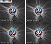 |
Fig. 2. Predictions of the total solar eclipse by the COCONUT model in the quasi-steady regime. Each figure corresponds to the corona prediction for different magnetogram files from Figure 1. The solar surface is coloured with the radial magnetic field values saturated to [−4,4]G. The magnetic field lines are overplotted on the eclipse image. The blue lines indicate the directions of the selected streamers based on the eclipse image. The red lines correspond to the direction of the same streamers as modelled by COCONUT simulations. Eclipse image credits: Eclipse team of Nanjing University – Wu, Sizhe (photographer); Li, Yihua; Huang, Yuhao; Lao, Qinghui; Cheng, Xin; Qu, Zhongquan. |
On the east limb, we chose regions 1 and 4 in the figure, while on the west limb, regions 2 and 3 showed the strongest features. The signatures near the poles were difficult to distinguish and poorly reconstructed by the magnetic field lines in the COCONUT simulations. Therefore, we decided not to focus on these areas, as they would not allow us to assess the performance of the COCONUT model. First, we considered the steamers on the east limb. Steamer 1 in COCONUT was modelled closely to the observed one, but the streamer direction is different. For streamer 4, on the other hand, the observed and simulated streamer directions are parallel, but the locations are not close to each other. On the west limb, regions 2 and 3 were modelled closely to the observations. The simulation results on March 28 do no change significantly because the eclipse date is still 11 days away, and the new information provided by the updated magnetogram is not yet accurate enough to improve the prediction for April 8. On April 3, the magnetic field configuration differed slightly in the centre of the disk and the eastern part. The resulting streamers are slightly more aligned with the observed structures than in the previous case. On the eclipse day, the magnetic field appears to be quite different across the entire disk. This means that the solar surface magnetic field evolved significantly over the 5 days between April 3 and April 8. The west limb is more accurate regarding the location and direction of the streamers. On the east limb, however, there is no significant improvement.
4.2. Dynamic simulations
4.2.1. Daily updated cadence
The predictions of the total solar eclipse we present in this section were performed using the time-evolving COCONUT regime. In this regime, the input magnetograms were updated to yield time-dependent inner boundary conditions. First, we updated the magnetograms daily to obtain information on the inner boundary similar to that in the quasi-steady regime. In this case, we obtained a continuously updated corona within the prediction window; however, we only plot the snapshots corresponding to the same days as in the quasi-steady case for comparison purposes. Figure 3 shows the modelled corona. The figure is arranged similarly to figure 2. The eclipse image is overlaid with magnetic field lines from time-evolving COCONUT simulations. The first image, corresponding to the predictions driven by the magnetogram observed on March 21, is similar to the image from the quasi-steady regime. On March 28 and April 3, steamer region 2 is less well aligned with the one in the eclipse image than that on March 21. All other streamers remain oriented in a manner similar to the previous date. The direction of this streamer also differs from that of the other dates in the quasi-steady regime. On April 8, the two simulated streamers on the west limb are well aligned with the observed streamers. The two streamers on the east limb, however, seem to approach each other. Streamer 4 is parallel to the direction of the corresponding streamer in the eclipse image. In contrast, the direction of streamer 1 appears to agree less well with the one observed on April 3. On the west limb, the quasi-steady and dynamic modelling regimes differ, while on the east limb, both regimes perform poorly. The two simulated streamers are in the correct places, but their direction seems different. The maximum solar activity means that distinguishing between different loops and streamers is extremely difficult, and this might lead to errors when estimating the directions of the streamers in the eclipse images.
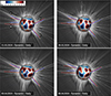 |
Fig. 3. Predictions of the total solar eclipse by the COCONUT model in the dynamic regime with daily updated magnetograms. Each figure corresponds to the corona prediction for different magnetogram files from Figure 1. The solar surface is coloured with the radial magnetic field values saturated to [−4,4] G. The magnetic field lines are overplotted on the eclipse image. The blue lines indicate the directions of the selected streamers based on the eclipse image. The red lines correspond to the direction of the same streamers as modelled by COCONUT simulations. Eclipse image credits: Eclipse team of Nanjing University – Wu, Sizhe (photographer); Li, Yihua; Huang, Yuhao; Lao, Qinghui; Cheng, Xin; Qu, Zhongquan. |
4.2.2. Hourly update cadence
This section presents results from the time-evolving COCONUT simulations that were obtained by updating the inner boundary conditions at an hourly cadence. Hence, 601 magnetograms were retrieved and pre-processed for this simulation. This simulation was performed using 270 CPUs on the big-memory nodes of the WICE cluster at VSC, with each CPU allocated 2000 MB of memory storage. It ran approximately 60 times faster than the real-time coronal evolution, completing a 600-hour physical period by just about 10 hours of computational wall-clock time.
As in the previous two cases, Figure 4 shows the results for the modelled total solar eclipse coronal configuration corresponding to March 21, March 28, April 3, and April 8. The comparison of the results in this case with those in the dynamic simulations with updated inner boundary conditions at a daily cadence shows that the results are similar, with only minimal differences. This is somewhat surprising because, considering the maximum solar activity, we would expect different coronal configurations with a higher updating frequency of the inner boundary magnetic field. When the photospheric magnetic field is updated hourly, all the available observational information is used to drive the dynamic solar corona. The magnetic field evolves rapidly on the solar surface near solar maximum. Because of the applied pre-processing of the magnetic field and the obtained smoothed magnetic maps, however, the changes in the modelled total solar corona are not as significant for the magnetograms with a 24-hour cadence or a 1-hour cadence. As a result, the results of hourly dynamic simulations are not significantly different from those of daily simulations.
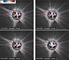 |
Fig. 4. Predictions of the total solar eclipse by the COCONUT model in the dynamic regime with hourly updated magnetograms. Each figure corresponds to the corona prediction for different magnetogram files from Figure 1. The solar surface is coloured with the radial magnetic field values saturated to [−4,4]G. The magnetic field lines are overplotted on the eclipse image. The blue lines indicate the directions of the selected streamers based on the eclipse image. The red lines correspond to the direction of the same streamers as modelled by COCONUT simulations. Eclipse image credits: Eclipse team of Nanjing University – Wu, Sizhe (photographer); Li, Yihua; Huang, Yuhao; Lao, Qinghui; Cheng, Xin; Qu, Zhongquan. |
4.2.3. Post eclipse analysis
The magnetograms show that the photospheric magnetic field configuration changes significantly on April 8 compared to April 3. Moreover, in the synoptic magnetograms, the region behind the east limb has not been updated for 14 days. Therefore, after the total solar eclipse, we used a magnetic field configuration on April 10 to model the solar corona and show Earth’s field of view as it would appear on April 8. In this way, we would be able to determine whether the additional observations on the east limb affect the modelled profile. The results are given in Figure 5. The figures are arranged similarly to the previous figures that illustrated the simulation results. The left panels shows the results for the quasi-steady simulation. The middle and right panels show the results for the dynamic simulations, with the boundaries driven by a daily or hourly cadence for updating magnetic field information. The streamer directions in all three types of simulations are similar. The west limb is modelled well, similar to previous cases. Significant differences occur between the modelled magnetic field configuration on the east limb using magnetograms observed before April 8 and those observed on April 10, however. There is a tendency of the two clear streamers to converge towards each other in the simulations corresponding to April 8. On April 10, the two separate streamers cannot be distinguished. There is one clear streamer between the previously modelled two streamers, close to region 4 in our original notation.
 |
Fig. 5. Predictions of the total solar eclipse by the COCONUT model with the magnetogram observed on April 10 in the quasi-steady, dynamic daily cadence and dynamic hourly regimes. The solar surface is coloured with the radial magnetic field values saturated to [−4,4] G. The magnetic field lines are overplotted on the eclipse image. The blue lines indicate the directions of the selected streamers based on the eclipse image. The red lines correspond to the direction of the same streamers as modelled by COCONUT simulations. Eclipse image credits: Eclipse team of Nanjing University – Wu, Sizhe (photographer); Li, Yihua; Huang, Yuhao; Lao, Qinghui, Cheng, Xin; Qu, Zhongquan. |
4.3. White-light images and polarised brightness
In addition to the corona validation technique suggested by Wagner et al. (2022), which was introduced previously in this section, we generated synthetic WL images to qualitatively compare the modelled data with the observed image. Next, we also compared the modelled polarised brightness to the observed one quantitatively to introduce the most comprehensive assessment of the predictive capabilities of the COCONUT coronal model.
4.3.1. Synthetic white-Light images
The synthetic WL images were generated from COCONUT simulations with the software FoMo. The code FoMo (Van Doorsselaere et al. 2016) WL extension (Sorokina et al. 2025) allows for computing WL synthetic data from arbitrary numerical models. The FoMo WL tool operates with data cubes or simulation snapshots in popular data formats. The forward-modelling procedure involves interpolating the plasma density from the original simulation grid to a Cartesian grid in the observation reference frame. Two rotation angles set the observer’s field of view (FOV). The resolution is user-defined. Thus, the synthetic image resolution and the orientation of its FOV can be tuned to the real instrument specifications or set for user analysis. Using the Thomson scattering theory, we converted the interpolated data into radiant intensity, which was integrated along the line of sight (LOS) to produce synthetic observations. FoMo uses open-source software (written in C++ and Python) to process the data and can run in parallel on multiple processors on high-performance computing systems. Details on installing and using the FoMo WL tool are available at GitHub: FoMo2.
Figure 6 shows the observed image on the left and the synthetic WL images created from COCONUT simulations. The middle panel corresponds to the simulation snapshot driven by the magnetograms up to the total solar eclipse time, and the right panel represents the simulation snapshot corresponding to the eclipse view from Earth, driven by the magnetogram observed up to 10.04.2024. Both simulations are driven in the dynamic regime, with daily updated magnetograms. The synthetic WL images were also generated for the other simulations presented in the previous section, but we only present the daily updated regime results because they yielded slightly better results than steady driving and similar results to the hourly updated simulations.
 |
Fig. 6. Eclipse and synthetic WL images generated from the COCONUT simulations performed with the magnetogram observed on April 8, 2024 and April 10, 2025. The two COCONUT simulations were performed in the dynamic regime with daily updated magnetograms. Eclipse image credits: Eclipse team of Nanjing University - Wu, Sizhe (photographer); Li, Yihua; Huang, Yuhao; Lao, Qinghui; Cheng, Xin; Qu, Zhongquan. |
Two streamers are visible in the west region and a prominent streamer in the south-west region, which are replicated in the synthetic images. Therefore, the west limb is modelled well compared to the real image. A region with a higher brightness lies closer to the south Pole, where significant features were observed in the eclipse image. The streamer is less pronounced in the synthetic images than in the observed eclipse image. The middle and right panels on the east limb are also significantly different. The synthetic WL image in the middle panel shows two narrow streamers near the equator. In the right panel, these streamers merge and blend into a larger streamer. This is due to new information about the emerging magnetic activity observed in the magnetograms after the eclipse date. The east limb is better modelled by the configuration in the right panel; thus, including the magnetic field information from the back of the Sun improved the modelled image.
The total solar eclipse was also modelled by the MAS model (Downs et al. 2025). The authors began making predictions on March 16, 2025, and also performed post-eclipse simulations on April 15, 2025. The methods and techniques used by the MAS model were significantly different from those used by COCONUT. Namely, they used the data assimilation method for integrating the Polarimetric and Helioseismic Imager (PHI) (Solanki et al. 2020) data on the Solar Orbiter into HMI magnetograms, and performed the surface flux transport (SFT) (Caplan et al. 2025) (model for creating the inner boundary magnetic field, while COCONUT used GONG input magnetograms filtered with spherical harmonics. Since the total solar eclipse occurred during the earlier development stage of COCONUT, we investigated its modelling capabilities with a simplified approach. We used a low-resolution domain with roughly 380 000 elements, as mentioned before, while the MAS model used ∼52 million elements. Additionally, our input magnetic field was heavily smoothed out, with a strength in the range ∼ ± 20 G, compared to ∼ ± 100 G used in the MAS input magnetic field maps. The synthetic WL images generated from MAS simulation results resolve structures in more detail than the COCONUT synthetic WL images, given in Fig. 6. This is largely due to the resolution used in the simulations and WL generation tools. The strong streamers were modelled reasonably well and fast, however. Each simulation took ∼20 minutes on 144 CPUs.
4.3.2. Polarised brightness
The modelled corona result was quantitatively compared to the observations by examining the normalised polarised brightness along the radial slit. Figure 7 compares the syntetic WL image produced from COCONUT simulation, driven by daily updated magnetograms, and the observation by the STEREO A/COR2 (Kaiser et al. 2008) around the time of the eclipse on 2024 Apr 8 at 19:03:45. The FOV of the synthetic image matches that of COR2-A when the separation angle between the Earth and the coronagraph is 10 degrees (see the right panel in Figure 7). The dashed white circle is drawn at 3 R⊙ and the radial slit is plotted in the panels in cyan along 315°. Here and below, the angle of zero degrees corresponds to the westernmost point on the circle and increases counterclockwise. The vertical axis in both images is aligned to the solar rotation axis, and the top of the image corresponds to the solar north pole. In the synthetic image, we hide the area below 2.3 R⊙ with a semi-transparent mask. The coronal configuration differs slightly from the observed eclipse image from Earth due to the different viewing locations (see the right panel in Figure 7). The north pole is oversaturated in the COCONUT simulation result, while it appears somewhat dimmed in the observations. The prominent streamer is present on the east limb in the observation and the COCONUT synthetic image. The enhanced region at the south pole is wider in the COCONUT simulation compared to the observation. The western limb is also well reproduced.
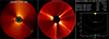 |
Fig. 7. Synthetic WL image generated from COCONUT with daily updated magnetograms up to the total solar eclipse for the STEREO A FOV and a real STEREO A/COR2 image are given in the first and second panels, respectively. The location of STEREO A with respect to Earth is plotted in the third panel. |
For a more detailed comparison, we considered the shape of the normalised polarised brightness profiles obtained during the observations and after forward-modelling. The calibrated observational data for comparison were extracted using the standard IDL/secchi_prep routine. Figure 8 compares the latitudinal profiles at 3 R⊙, shown as a dashed white circle in Figure 7. The normalised polarised brightness profiles also suggest that the north pole is completely oversaturated compared to the COR2 observations. The streamer between 150° and 200° is present in the COCONUT simulation and in the COR2 image, but the COCONUT image is undersaturated. The streamer near the south pole is spread out in the COCONUT simulation, and the profile observed is well recovered after the 315° region. The enhanced profiles near the poles in the simulations might be due to a heavily processed input magnetic map affecting the heating profile. The comparison in Figure 8 confirms the conclusion of the qualitative comparison from Figure 7.
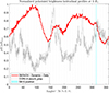 |
Fig. 8. Normalised polarised brightness from COR2-A (data extracted with the standard secchi_prep routine) and COCONUT dynamic simulation with daily updated magnetograms. The polarised brightness is given for the entire latitudinal range at a distance of 3 R⊙. The slit position denoted by S in Figure 7 is indicated with the vertical cyan line. |
Figure 9 compares the radial profiles along the line S at 315°, shown as a cyan line in Figure 7. The radial profiles of the polarised brightness in the observed image and the COCONUT simulation agree well.
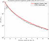 |
Fig. 9. Normalised polarised brightness along the slit denoted by S in Figure 7, corresponding to 315°. The from COR2-A (data extracted with the standard secchi_prep routine) and COCONUT synthetic polarised brightness is plotted up to 10 R⊙. |
5. Conclusions
The total solar eclipse on April 8, 2024, was used to validate the COCONUT coronal model. Previously, only the simple, polytropic version of the COCONUT model was used to assess the low corona configuration of the Sun. This study used the full MHD version of COCONUT, which includes the source and sink terms and provides a more detailed description of the heating, thermal conduction, and radiative loss processes near the Sun. Due to the high solar activity during the eclipse, highly processed maps were used with a low-resolution grid for the computations. The total solar corona predictions started on March 21, 2024, and were run in different regimes. First, the predictions were performed in the quasi-steady mode. Steady simulations were run daily before the total solar eclipse, and their evolution was monitored over 19 days.
Each of these simulations took ∼20 minutes on four nodes with 36 cores each on the Genius cluster of the Flemish supercomputer centre. Then, after the eclipse, time-dependent simulations were performed using the same daily updated magnetograms as those used for the quasi-steady predictions. The magnetograms were interpolated and fed into the COCONUT simulation as time-evolving inner boundary conditions. The last regime we investigated considered the time-dependent dynamic simulations with hourly updated magnetograms. In this way, we investigated the effect of dynamic driving of the boundary and the cadence of the inner boundary.
We used various techniques available in the literature to validate the obtained results. Since the input magnetic maps were highly processed and the domain resolution was low, we chose to use multiple validation techniques. First, we examined the configuration of the magnetic streamers in the modelled solar corona and overlaid the magnetic field lines onto the total solar eclipse image. This was done for both quasi-steady and dynamic simulations with low and high cadence. The most similar configuration was achieved in the dynamic simulations. When we increased the cadence of the inner boundary conditions, the results did not notably improve, however, likely due to the strong pre-processing of the maps.
We also performed simulations that included the magnetograms observed after the total solar eclipse. The east limb was modelled differently due to the updated magnetic field information from the back of the Sun. Based on the comparison of the magnetic field configuration of the solar corona, we used only dynamic simulations driven by a daily cadence for the following validation techniques. This implied the synthetic WL images and normalised polarised brightness profiles. This analysis showed that the prominent streamers were reconstructed well on the west limb, and the streamer location on the east limb was affected by including the information from the back of the Sun. The normalised polarised brightness image at 3 R⊙ confirmed the comparison of the latitudinal distribution of the enhanced regions in the observed and modelled images. The normalised polarised brightness along 315° radial slit showed that the profiles of the observed and modelled corona agreed well.
It was challenging to predict the total solar eclipse of 2024 because of the high solar activity and the strong magnetic field regions on the solar surface. It was essential to use multiple validating techniques to assess the model performance and determine the role of processing the input data in the obtained results. Even though the pronounced streamers were reconstructed in the model, the main limitation of the model remains the lack of a detailed magnetic field configuration at the inner boundary. Improving the robustness of the COCONUT model is the next step in its development. For future work, we intend to investigate the relation between the processed magnetic field and the generated synthetic while-light images in the simulations. Additionally, we intend to perform coronal modelling with a less strongly processed magnetogram at a higher-resolution computational domain to reconstruct the observed features in more detail and avoid smoothing them over vast regions.
Acknowledgments
This research has received funding from the European Union’s Horizon 2020 research and innovation programme under grant agreement No 870405 (EUHFORIA 2.0) and the ESA project “Heliospheric Modelling Techniques” (Contract No. 4000133080/20/NL/CRS). These results were also obtained in the framework of the projects C16/24/010 (C1 project Internal Funds KU Leuven), AFOSR FA9550-18-1-0093, G0B5823N and G002523N (FWO-Vlaanderen), and SIDC Data Exploitation (ESA Prodex-12). The computational resources and services used in this work were provided by the VSC-Flemish Supercomputer Center, funded by the Research Foundation Flanders (FWO) and the Flemish Government-Department EWI. SP also acknowledges funding by the European Union. Views and opinions expressed are, however, those of the author(s) only and do not necessarily reflect those of the European Union or ERCEA. Neither the European Union nor the granting authority can be held responsible for them. This project (Open SESAME) has received funding under the Horizon Europe programme (ERC-AdG agreement No 101141362). The STEREO/SECCHI data used here are produced by an international consortium of the Naval Research Laboratory (USA), Lockheed Martin Solar and Astrophysics Laboratory (USA), NASA Goddard Space Flight Center (USA), Rutherford Appleton Laboratory (UK), University of Birmingham (UK), Max-Planck-Institut für Sonnensystemforschung (Germany), Centre Spatial de Liège (Belgium), Institut d’Optique Théorique et Appliqué (France), and Institut d’Astrophysique Spatiale (France).
References
- Baratashvili, T., Brchnelova, M., Linan, L., Lani, A., & Poedts, S. 2024, A&A, 690, A184 [NASA ADS] [CrossRef] [EDP Sciences] [Google Scholar]
- Baratashvili, T., Popescu Braileanu, B., Bacchini, F., Keppens, R., & Poedts, S. 2025, A&A, 694, A306 [NASA ADS] [CrossRef] [EDP Sciences] [Google Scholar]
- Brchnelova, M., Kuźma, B., Perri, B., et al. 2022a, ApJS, accepted [Google Scholar]
- Brchnelova, M., Zhang, F., Leitner, P., et al. 2022b, J. Plasma Phys., 88, 905880205 [NASA ADS] [CrossRef] [Google Scholar]
- Caplan, R. M., Stulajter, M. M., Linker, J. A., et al. 2025, ApJS, 278, 24 [Google Scholar]
- Chorin, A. J. 1997, J. Comput. Phys., 135, 118 [NASA ADS] [CrossRef] [Google Scholar]
- Dedner, A., Kemm, F., Kröner, D., et al. 2002, J. Comput. Phys., 175, 645 [Google Scholar]
- Downs, C., Linker, J. A., Caplan, R. M., et al. 2025, Science, 388, 1306 [Google Scholar]
- Kaiser, M. L., Kucera, T. A., Davila, J. M., et al. 2008, Space Sci. Rev., 136, 5 [Google Scholar]
- Kimpe, D., Lani, A., Quintino, T., Poedts, S., & Vandewalle, S. 2005, in Recent Advances in Parallel Virtual Machine and Message Passing Interface, eds. B. Di Martino, D. Kranzlmüller, & J. Dongarra (Berlin, Heidelberg: Springer, Berlin Heidelberg), 520 [Google Scholar]
- Kuźma, B., Brchnelova, M., Perri, B., et al. 2023, ApJ, 942, 31 [CrossRef] [Google Scholar]
- Lani, A., Quintino, T., Kimpe, D., et al. 2005, in Computational Science - ICCS 2005, eds. V. S. Sunderam, G. D. van Albada, P. M. A. Sloot, & J. J. Dongarra, (Berlin, Heidelberg: Springer, Berlin Heidelberg), 279 [Google Scholar]
- Lani, A., Quintino, T., Kimpe, D., et al. 2006, Sci. Program., 14 [Google Scholar]
- Lani, A., Villedieu, N., Bensassi, K., et al. 2013, in AIAA 2013-2589, 21th AIAA CFD Conference, San Diego (CA) [Google Scholar]
- Lani, A., Yalim, M. S., & Poedts, S. 2014, Comput. Phys. Commun., 185, 2538 [NASA ADS] [CrossRef] [Google Scholar]
- Mikic, Z., & Linker, J. A. 1996, AIP Conf. Proc., 382, 104 [CrossRef] [Google Scholar]
- Mikić, Z., Linker, J. A., Schnack, D. D., Lionello, R., & Tarditi, A. 1999, Phys. Plasmas, 6, 2217 [Google Scholar]
- Perri, B., Leitner, P., Brchnelova, M., et al. 2022, ApJ, 936 [Google Scholar]
- Pinto, R. F., & Rouillard, A. P. 2017, ApJ, 838, 89 [NASA ADS] [CrossRef] [Google Scholar]
- Pomoell, J., & Poedts, S. 2018, J. Space Weather Space Clim., 8, A35 [NASA ADS] [CrossRef] [EDP Sciences] [Google Scholar]
- Réville, V., Folsom, C. P., Strugarek, A., & Brun, A. S. 2016, ApJ, 832, 145 [CrossRef] [Google Scholar]
- Réville, V., Velli, M., Panasenco, O., et al. 2020, ApJS, 246, 24 [Google Scholar]
- Schatten, K. H., Wilcox, J. M., & Ness, N. F. 1969, Sol. Phys., 6, 442 [Google Scholar]
- Solanki, S. K., del Toro Iniesta, J. C., Woch, J., et al. 2020, A&A, 642, A11 [NASA ADS] [CrossRef] [EDP Sciences] [Google Scholar]
- Sorokina, D., Van Doorsselaere, T., Lloveras, D. G., Linan, L., & Poedts, S. 2025, A&A, 701, A166 [NASA ADS] [CrossRef] [EDP Sciences] [Google Scholar]
- Usmanov, A. V., Goldstein, M. L., & Matthaeus, W. H. 2014, ApJ, 788, 43 [Google Scholar]
- Usmanov, A. V., Matthaeus, W. H., Goldstein, M. L., & Chhiber, R. 2018, ApJ, 865, 25 [Google Scholar]
- van der Holst, B., Sokolov, I. V., Meng, X., et al. 2014, ApJ, 782, 81 [Google Scholar]
- Van Doorsselaere, T., Antolin, P., Yuan, D., Reznikova, V., & Magyar, N. 2016, Front. Astron. Space Sci., 3, 4 [Google Scholar]
- Wagner, A., Asvestari, E., Temmer, M., Heinemann, S. G., & Pomoell, J. 2022, A&A, 657, A117 [NASA ADS] [CrossRef] [EDP Sciences] [Google Scholar]
- Wang, H. P., Poedts, S., Lani, A., et al. 2025a, A&A, 694, A234 [NASA ADS] [CrossRef] [EDP Sciences] [Google Scholar]
- Wang, H. P., Poedts, S., Lani, A., et al. 2025b, A&A, 702, A37 [NASA ADS] [CrossRef] [EDP Sciences] [Google Scholar]
- Wang, H. P., Yang, L. P., Poedts, S., et al. 2025c, ApJS, 278, 59 [Google Scholar]
- Yalim, M. S., Vanden Abeele, D., Lani, A., Quintino, T., & Deconinck, H. 2011, J. Comput. Phys., 230, 6136 [NASA ADS] [CrossRef] [Google Scholar]
- Zhukov, A. N., Thizy, C., Galano, D., et al. 2025, arXiv e-prints [arXiv:2509.00253] [Google Scholar]
Appendix A: Areas of interest in the input maps
Figure A.1 shows the calculated difference between the processed radial magnetic field values of the consecutive input magnetic field data given in Figure 1. The same boxes as in Figure 1 are plotted on top of the difference plots. Box 1 shows the difference between the input magnetogram observed on March 28 and March 21. Figure A.1 shows that the strongest differences are present near the right edge of the box, where the magnetic field is also the strongest in the input magnetogram shown in Figure 1. However, when considering the structure of the magnetic field configuration, we notice that near the left edge of the box, the slightly enhanced differences indicated lead to a change in the magnetic field structure in the input magnetogram. Thus, we also included this region in this box, rather than limiting it only to the strongest part. As a result, we considered both the magnetic field configuration in the input maps and the calculated differences between consecutive maps to identify the three areas of interest where the most change occurs over time.
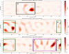 |
Fig. A.1. The difference between the smoothed input magnetic field data between the consecutive dates shown in Figure 1 of the paper. The title indicates the dates between which the difference was calculated. |
All Figures
|
Fig. 1. Original GONG (upper panels) and pre-processed input magnetograms (lower panels) for March 21, March 28, April 3 and April 8. The colour maps are saturated to the [−20, 20] G range. All maps are rotated so that they are aligned with the Earth’s view angle as of April 8, 2024. Squares 1, 2 and 3 represent the areas of interest. |
| In the text | |
|
Fig. 2. Predictions of the total solar eclipse by the COCONUT model in the quasi-steady regime. Each figure corresponds to the corona prediction for different magnetogram files from Figure 1. The solar surface is coloured with the radial magnetic field values saturated to [−4,4]G. The magnetic field lines are overplotted on the eclipse image. The blue lines indicate the directions of the selected streamers based on the eclipse image. The red lines correspond to the direction of the same streamers as modelled by COCONUT simulations. Eclipse image credits: Eclipse team of Nanjing University – Wu, Sizhe (photographer); Li, Yihua; Huang, Yuhao; Lao, Qinghui; Cheng, Xin; Qu, Zhongquan. |
| In the text | |
|
Fig. 3. Predictions of the total solar eclipse by the COCONUT model in the dynamic regime with daily updated magnetograms. Each figure corresponds to the corona prediction for different magnetogram files from Figure 1. The solar surface is coloured with the radial magnetic field values saturated to [−4,4] G. The magnetic field lines are overplotted on the eclipse image. The blue lines indicate the directions of the selected streamers based on the eclipse image. The red lines correspond to the direction of the same streamers as modelled by COCONUT simulations. Eclipse image credits: Eclipse team of Nanjing University – Wu, Sizhe (photographer); Li, Yihua; Huang, Yuhao; Lao, Qinghui; Cheng, Xin; Qu, Zhongquan. |
| In the text | |
|
Fig. 4. Predictions of the total solar eclipse by the COCONUT model in the dynamic regime with hourly updated magnetograms. Each figure corresponds to the corona prediction for different magnetogram files from Figure 1. The solar surface is coloured with the radial magnetic field values saturated to [−4,4]G. The magnetic field lines are overplotted on the eclipse image. The blue lines indicate the directions of the selected streamers based on the eclipse image. The red lines correspond to the direction of the same streamers as modelled by COCONUT simulations. Eclipse image credits: Eclipse team of Nanjing University – Wu, Sizhe (photographer); Li, Yihua; Huang, Yuhao; Lao, Qinghui; Cheng, Xin; Qu, Zhongquan. |
| In the text | |
|
Fig. 5. Predictions of the total solar eclipse by the COCONUT model with the magnetogram observed on April 10 in the quasi-steady, dynamic daily cadence and dynamic hourly regimes. The solar surface is coloured with the radial magnetic field values saturated to [−4,4] G. The magnetic field lines are overplotted on the eclipse image. The blue lines indicate the directions of the selected streamers based on the eclipse image. The red lines correspond to the direction of the same streamers as modelled by COCONUT simulations. Eclipse image credits: Eclipse team of Nanjing University – Wu, Sizhe (photographer); Li, Yihua; Huang, Yuhao; Lao, Qinghui, Cheng, Xin; Qu, Zhongquan. |
| In the text | |
|
Fig. 6. Eclipse and synthetic WL images generated from the COCONUT simulations performed with the magnetogram observed on April 8, 2024 and April 10, 2025. The two COCONUT simulations were performed in the dynamic regime with daily updated magnetograms. Eclipse image credits: Eclipse team of Nanjing University - Wu, Sizhe (photographer); Li, Yihua; Huang, Yuhao; Lao, Qinghui; Cheng, Xin; Qu, Zhongquan. |
| In the text | |
|
Fig. 7. Synthetic WL image generated from COCONUT with daily updated magnetograms up to the total solar eclipse for the STEREO A FOV and a real STEREO A/COR2 image are given in the first and second panels, respectively. The location of STEREO A with respect to Earth is plotted in the third panel. |
| In the text | |
|
Fig. 8. Normalised polarised brightness from COR2-A (data extracted with the standard secchi_prep routine) and COCONUT dynamic simulation with daily updated magnetograms. The polarised brightness is given for the entire latitudinal range at a distance of 3 R⊙. The slit position denoted by S in Figure 7 is indicated with the vertical cyan line. |
| In the text | |
|
Fig. 9. Normalised polarised brightness along the slit denoted by S in Figure 7, corresponding to 315°. The from COR2-A (data extracted with the standard secchi_prep routine) and COCONUT synthetic polarised brightness is plotted up to 10 R⊙. |
| In the text | |
|
Fig. A.1. The difference between the smoothed input magnetic field data between the consecutive dates shown in Figure 1 of the paper. The title indicates the dates between which the difference was calculated. |
| In the text | |
Current usage metrics show cumulative count of Article Views (full-text article views including HTML views, PDF and ePub downloads, according to the available data) and Abstracts Views on Vision4Press platform.
Data correspond to usage on the plateform after 2015. The current usage metrics is available 48-96 hours after online publication and is updated daily on week days.
Initial download of the metrics may take a while.