| Issue |
A&A
Volume 705, January 2026
|
|
|---|---|---|
| Article Number | A144 | |
| Number of page(s) | 13 | |
| Section | Extragalactic astronomy | |
| DOI | https://doi.org/10.1051/0004-6361/202556558 | |
| Published online | 14 January 2026 | |
Early identification of optical tidal disruption events
A science module for the Fink broker
1
IRAP, Université de Toulouse, CNRS, CNES, UPS Toulouse, France
2
Institute of Physics of the Czech Academy of Sciences Na Slovance 1999/2 182 00 Prague 8, Czech Republic
3
The Oskar Klein Centre, Department of Astronomy, Stockholm University AlbaNova SE-10691 Stockholm, Sweden
4
European Space Agency (ESA), European Space Astronomy Centre (ESAC) Camino Bajo del Castillo s/n 28692 Villanueva de la Cañada Madrid, Spain
5
Université Clermont Auvergne, CNRS, LPCA Clermont-Ferrand F-63000, France
6
Université Paris-Saclay, CNRS/IN2P3, IJCLab Orsay, France
7
Lomonosov Moscow State University, Sternberg Astronomical Institute Universitetsky 13 Moscow 119234, Russia
8
Centre for Astrophysics and Supercomputing, Swinburne University of Technology Mail Number H29 PO Box 218 31122 Hawthorn VIC, Australia
9
ARC Centre of Excellence for Gravitational Wave Discovery (OzGrav) John St Hawthorn VIC 3122, Australia
★ Corresponding authors: This email address is being protected from spambots. You need JavaScript enabled to view it.
; This email address is being protected from spambots. You need JavaScript enabled to view it.
Received:
23
July
2025
Accepted:
20
November
2025
Abstract
Context. The detection of tidal disruption events (TDEs) is one of the key science goals of large optical time-domain surveys such as the Zwicky Transient Facility (ZTF) and the upcoming Vera C. Rubin Observatory Legacy Survey of Space and Time. Automated and reliable classification pipelines that can select promising candidates in real time are required to identify TDEs in the vast alert streams produced by these surveys, however.
Aims. We developed a module within the FINK alert broker to identify TDEs during their rising phase. The module was built to autonomously operate within the ZTF alert stream and to produce a list of candidates every night, enabling spectral and multiwavelength follow-up near peak brightness.
Methods. All rising alerts were submitted to selection cuts and feature extraction using the RAINBOW multiband light-curve fit. Best-fit values were used as input to train an XGBoost classifier with the goal of identifying TDEs. The training set was constructed using ZTF observations for objects with available classification in the Transient Name Server. Finally, candidates for which the probability was high enough were inspected visually.
Results. The classifier achieved 76% recall, which indicates a strong performance in early-phase identification, despite the limited available information before the peak. Out of the known TDEs that passed the selection cuts, half were flagged as TDEs before they had risen half the way. This proves that an early classification is possible. Additionally, new candidates were identified by applying the classifier on archival data, including a likely repeated TDE and some potential TDEs that occurred in active galaxies. The module is implemented in the FINK alert-processing framework and each night reports a small number of candidates to dedicated communication channels through a user-friendly interface for manual vetting and potential follow-up.
Key words: black hole physics / methods: data analysis / techniques: photometric / surveys
These authors contributed equally to this work and share first authorship.
© The Authors 2026
 Open Access article, published by EDP Sciences, under the terms of the Creative Commons Attribution License (https://creativecommons.org/licenses/by/4.0), which permits unrestricted use, distribution, and reproduction in any medium, provided the original work is properly cited.
This article is published in open access under the Subscribe to Open model. This email address is being protected from spambots. You need JavaScript enabled to view it. to support open access publication.
1. Introduction
Tidal disruption events (TDEs; Hills 1975, 1988; Rees 1988; Bade et al. 1996; Gezari 2021) correspond to the destruction of a star that passes within the tidal radius of a supermassive black hole because the intense tidal forces overcome the stellar self-gravity. Depending on the properties of the star, the black hole, and their relative trajectories, this disruption can be complete or only partial. In the latter case, the event can be repeated. The typical observational behavior of TDEs is a sudden rise in the emission of the galactic nucleus that is well described by a thermal continuum (for nonjetted TDEs), followed by a decay over a few months to a few years that is approximately consistent with a t−5/3 power-law decay (e.g., Rees 1988). This general behavior is seen at all wavelengths, but with different timing and temperature properties.
These events are relatively rare, with a rate of about 10−5 galaxy−1 year−1 (e.g., Yao et al. 2023). The first known TDEs were discovered in soft X-rays (e.g. Bade et al. 1996) by the ROentgen SATellite (ROSAT, Pfeffermann et al. 1986). Most of the current sample of TDEs was however provided by optical surveys, such as the Zwicky Transient Facility (ZTF; Bellm 2014), because they monitor the sky intensely with a cadence that is optimized for finding these transient events. TDEs have also been discovered in the radio (e.g., Bloom et al. 2011) and infrared (e.g., Masterson et al. 2024). The current sample contains about 150 TDEs at all wavelengths (e.g., Langis et al. 2025).
While the general picture of a bright months-long transient event is common to most wavelengths, the precise spectral and timing properties do not always match. Many questions remain unanswered about the multiwavelength counterparts of these events (e.g., Saxton et al. 2018) and about the precise emission mechanisms. One current hypothesis is that a central X-ray engine powers all TDEs (e.g., Dai et al. 2018), although X-ray emission is not always seen in these objects (e.g., Guolo et al. 2024).
To answer these questions and improve our understanding of the mechanisms at play in TDEs, there are mainly two different possible avenues of progress. The first avenue is the use of simulations (e.g., Guillochon & Ramirez-Ruiz 2013), which is particularly difficult for TDEs because of the general relativity effect, the prevalence of shocks and plasma effects in the hot ionized matter around the black hole, and the wide range of timescales and spatial scales needed to capture the entirety of the phenomenon. The other avenue is observational. It is possible to constrain the spectral-timing properties of these objects through systematic and rapid multiwavelength follow-up and by monitoring newly detected TDEs, especially during their rising phase. The study of these properties might allow us to constrain the current models, for example, by enabling population studies.
These observational approaches are particularly relevant now, with the advent of large-scale transient-focused missions such as the aforementioned ZTF, the recently launched Einstein Probe (Yuan et al. 2015), or the upcoming Vera C. Rubin Observatory Legacy Survey of Space and Time (LSST; Ivezić et al. 2019). These missions produce an unprecedented amount of data, and dedicated software and methods must be developed in order to ensure the identification of TDEs (or any other type of specific transients) in their data streams. TDE photometric candidate samples can be contaminated by various types of transients, including bright supernovae and superluminous supernovae, as well as high-accretion episodes in active galactic nuclei (AGNs). Ideally, the combination of spectral and photometric data is necessary to provide a definitive answer about the nature of a transient event. Spectral data are observationally expensive, however, and the community has therefore dedicated considerable effort to the development of photometric classification techniques.
Recently, several classifiers have been proposed to address the specific issue of optical TDE photometric classification. They are based on intrinsically different methods. FLEET (Gomez et al. 2023) relies on automatic host galaxy association and light-curve feature extraction to train a random forest classifier. It proposes two separate models that can classify early and full light curves. The ALeRCE broker (Förster et al. 2021) proposed to expand their previous multiclass classifier (Sánchez-Sáez et al. 2021) with 24 additional features that are designed to separate TDEs from other transients (Pavez-Herrera et al. 2025). They include the distance from the host, new fitting models, and color information. NEEDLE (Sheng et al. 2024) directly leverages the detection and reference images that are combined with photometric information from the alert packets to train a convolutional neural network. It comes in several versions, with or without usage of the host galaxy information. Finally, tdescore (Stein et al. 2024) extracts features by performing a Gaussian process assuming a linear evolution of the transient color. They are used together with the host galaxy information to train an XGBoost classifier (Chen & Guestrin 2016).
Although all classification pipelines can process early light curves in principle, only FLEET proposes an additional classifier dedicated to the identification of TDEs in their early phase. It proceeds by fitting a parametric model to light curves with a history shorter than 20 days and fixing the decay parameter such that the fit is effectively made for the rising part alone. This method offers a rapid classification with fewer data points, but it does not guarantee that the identification occurs before the peak luminosity of the source.
We focus on the identification of TDEs based on the rising part of their light curves alone. Our goal is to provide a reliable pre-maximum classifier that can be used to separate a stream of promising candidates to enable early follow-up. The classifier should not exclusively fine-tune its predictions based on the current sparse number of known TDEs, but should also remain compatible with our understanding of their possible characteristics. Hence, our aim is not to maximize purity, but completeness, such that the classifier can be used as an early warning tool to obtain as many promising candidates as possible directly from the alert stream. In particular, we developed a science module for the FINK broker, which will process the alert data stream after every night and report a list of candidates.
We introduce the FINK alert broker, which processes ZTF and Rubin LSST data, in Sect. 2. We then describe the design choices of our TDE early classification module in Sect. 3. We present the results in Sect. 4, including the efficiency of the classifier and a selection of candidates it found in the ZTF archive. Finally, we discuss this work in Sect. 5 and place it in context with other classifiers and the upcoming Rubin data.
2. The FINK alert broker
FINK is an astronomy community broker that processes time-domain alert streams and redirects relevant subsets of the data to science teams and follow-up facilities while also making the data accessible through its web-portal1 and data transfer service2 (Möller et al. 2021). The broker collects, filters, aggregates, enriches, and redistributes incoming data streams in real time. This is done through a series of filters and science modules that were developed by the community. Independent science teams are responsible for developing modules according to their specific scientific interests. When they are finalized, these modules are integrated in the broker, and real-time processing is centralized in dedicated infrastructures. FINK was conceived to process the full stream of alerts from the Vera C. Rubin Observatory (Ivezić et al. 2019) as part of the Rubin Community brokers3.
Since late 2019, FINK has been operating on the ZTF public stream (Bellm et al. 2019) as a precursor experiment for Rubin. The broker receives data from the difference-imaging analysis pipeline, which includes three image stamps, contextual information, and a 30-day photometric history within each alert package. Alerts that satisfy a set of quality criteria4 are then processed by FINK science modules, whose task is to add value and to thus help decipher the nature of the sources. These include cross-matches with major catalogs as well as statistics and machine-learning-based routines that transfer domain knowledge to each alert5. The range of science modules and the respective astrophysical subjects they address reflects the variety within the FINK community. This includes supernovae (SNe; Leoni et al. 2022; Möller & de Boissière 2020; Möller et al. 2025), kilonovae (Biswas et al. 2023), gamma-ray bursts (Masson & Bregeon 2024), microlensing (Ban et al. 2025), Solar System objects (Le Montagner et al. 2023), multiclass classifiers (Fraga et al. 2024), extragalactic hostless transients (Pessi et al. 2024), and anomaly detection6. Each science team has complete autonomy while developing their module, but the output of all modules is public and is therefore available to anyone using FINK. It is therefore crucial to clarify the hypothesis used in the development of each module, so that the community can make informed decisions regarding their output (e.g., class probabilities or candidate lists). The broker currently processes around 200 000 ZTF alerts per night. This number is expected to scale to 10 million when the LSST becomes operational.
The goal of this work is to give details on the development of the early TDE science module available in FINK. We describe the target candidates and the hypotheses used in its development in detail and thus enable others to either make informed follow-up decisions based on our list of candidates or inspire the development of alternative pipelines.
3. Early TDE module design
We developed a supervised classifier aimed at identifying rising TDEs in the ZTF alert stream. Below, we give details on the main steps that led to the final pipeline. They include selection cuts and identification of rising light curves (Sect. 3.1), feature extraction (Sect. 3.2), filtering and labeling (Sect. 3.3), and the classifier itself (Sect. 3.4).
3.1. Preprocesing
Starting from ZTF light curves available in FINK, we applied a set of filters to select relevant objects. The goal of this step is to take advantage of domain knowledge in order reduce the complexity of the input dataset to be shown to the machine-learning model.
First, we used a positional cross-match with SIMBAD (Wenger et al. 2000) and selected objects that were either absent from the catalog or were classified into categories that were broadly consistent with TDE host environments (e.g., extragalactic, lensing systems, transients, or active galaxies). Second, we excluded all known Solar System objects in the Minor Planet Center7 (MPC). Third, in order to limit the contamination from galactic objects, we also excluded all sources with galactic latitude |b|< 20°. For every remaining object, we extracted the complete ZTF light curves in the g and r bands from the FINK database that covered the time interval between November 2019 and February 2025.
We corrected the photometry of these objects for galactic extinction using the Schlegel et al. (1998) estimates of E(B − V) and the Gordon (2024) implementation of the Gordon et al. (2023) extinction law. We then converted the photometric measurements into fluxes using a magnitude zeropoint of 27.5, which gives the flux in so-called FLUXCAL units (Kessler et al. 2009). The flux values correspond to the brightness differences between the science and reference stamps. A positive value means that the transient in the science image is brighter than in the reference, and a negative value means a fainter object in the science stamp.
For each remaining light curve, we performed a sliding-window search to select all possible rising segments. To achieve this, we defined three time intervals at each data point (see Fig. A.1): a 100-day fitting window immediately preceding the data point, used to search for the rising TDE; a 100-day historical interval prior to the fitting window; and a pre-historical window including all data before that. Then, we applied the following criteria, which must be fulfilled simultaneously in each of these windows:
-
i
Fitting window
-
Rising in at least one band: Either the last detection in the band must be at least 2σ above the minimum flux in this band, or the linear regression slope across the entire time interval should be significantly positive (> 3σ).
-
Not decaying in any band: In each band, the last detection cannot be > 1σ below the maximum measured flux, and no point should be > 1σ below the immediately preceding one.
-
This window must contain at least five detections in total, with at least one in each band, and no more than one measurement with negative flux.
-
-
ii
Historical window: To exclude objects with persistent long-term activity, we only considered objects without detections in this time window.
-
iii
Pre-historical window: To further restrict the contamination from objects with a persistent large amplitude variability while still preserving the potential presence of repeated transient flashes, we allowed one detection with negative flux in this window at most. This criterion has proved to be efficient in suppressing objects that historically vary strongly in the current ZTF data, but further improvements on this criterion are the subject of a subsequent version of the module.
3.2. Feature extraction
Every rising interval, as defined above in (i), was submitted to a light-curve fit using a simple parametric function within the RAINBOW (Russeil et al. 2024a) framework. This approach assumes that the transient has a blackbody spectrum and describes its multicolor evolution through two independent parametric models, one model for the bolometric flux, and another model for the temperature. The optimized parameters constitute a highly discriminative feature set that has been proven effective in separating transient classes (Fraga et al. 2024). In particular, Russeil et al. (2024a) showed that among various transients, TDE classification benefits most from RAINBOW features because the spectral behavior of TDEs from broadband photometry is generally well-approximated by a blackbody.
We chose to model the bolometric flux evolution of the rising light curves with a simple logistic (sigmoid) function of the form
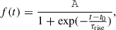 (1)
(1)
where τrise is the characteristic rise time, A is the amplitude, and t0 corresponds to the time of half-maximum. We also considered a constant temperature value throughout the rise T(t) = T.
This assumption of a constant temperature is often used when modeling TDEs because it is consistent with optical observations, especially during the rise. While a slight temperature evolution may be observed in later phases, the rise typically exhibits little to no temperature evolution (see, e.g., Hung et al. 2017; van Velzen et al. 2020). The logistic bolometric flux constitutes a simple but sufficient model given the simple behavior of TDEs on the rise and the cadence of the observations. Although other functional forms would have been equally accurate, it offers a low number of parameters and high computational stability.
Overall, our RAINBOW model has only four free parameters. This minimalist description enables early fits with a minimum of only five data points, while being sufficient to describe the rising part of most transients light curves. The lower panel of Fig. A.1 shows an example of this fit.
The RAINBOW package returns the following features from the fit, alongside their covariances: reference_time (t0), rise_time (τrise), temperature (T), amplitude (A), and r_chisq (reduced χ2). We also computed a value reflecting the sigmoid compression that was used to filter the data (see Sect. 3.3). We defined it as norm_rel_reference_time =(t0 − tlast)/τrise, with tlast the time of last detection.
From this set, we included only four relevant features to train the classifier. We selected T and τrise, which constitute the only physically discriminating features. In addition, we used the uncertainty associated with t0, e_reference_time as an additional informative feature that reflects the degree to which the fit is constrained. Finally, we included the mean angular distance (in pixels) to the nearest object in the ZTF reference image, distnr. This value was used as a proxy for the transient offset from the center of its host galaxy and served as an indicator of how nuclear the event is. When the host galaxy is well resolved, this feature can be particularly helpful in rejecting some off-nuclear transients such as SNe. However, distnr may become unreliable when the host is not detected in its quiescence state, which leads to associations with unrelated nearby objects, and consequently, to meaningless distnr values. To evaluate the usefulness of this feature, we trained the classifier in two variants, the nuclear version, which includes the feature and the broad version, that omits it.
3.3. Filtering and labeling
Prior to the training and classification, we applied an additional filtering step based on the output of the RAINBOW fit. Specifically, to avoid very poor fits (which would correspond to data that are clearly inconsistent with the single-temperature sigmoid model), we excluded the entries with r_chisq greater than 10. The entries with signal-to-noise ratios (defined as the parameter value divided by its uncertainty) lower than 1.5 in either rise time or temperature were also excluded. We also required norm_rel_reference_time to be between –10 and 0 to exclude overly compressed sigmoid fits (lower bound), as well as highly unconstrained sigmoid shapes whose center lies well after the last alert (upper bound).
For the training, we used the subset of all objects that were positionally coincident with the entries in the Transient Name Server8 (TNS) as of June 1, 2025, to which we applied the processing presented in Sects. 3.1, 3.2, and 3.3. In constructing a binary classifier, we constructed a set of positives (TDEs) and a set of negatives (others).
For the positives, we selected all TNS entries classified as TDEs, regardless of subtype, and added a few TDEs reported by Hammerstein et al. (2022) whose classification was not available in TNS at the time of writing. Because TNS classifications are dominated by SNe, as expected from their volumetric rates relative to other similar transients, we labeled as negatives all TNS objects that were not classified as TDEs, including 4823 that lacked any classification. This is justified by the rarity of TDEs among other possible types of impostors (AGN activity, cataclysmic variables, novae, etc.) that typically remain unclassified in TNS. It is reasonable to expect that TNS does not capture the full range of impostors encountered in the live-alert stream, which warrants caution when interpreting the model performance. Nevertheless, the resulting sample is expected to be complete enough for a careful extrapolation of results when in production.
This resulted in a training dataset with 8865 entries, only 42 of which were positives (known TDEs). Figure 1 shows the values of temperature and rise time obtained from RAINBOW for all entries in the dataset. TDEs tend to exhibit higher temperatures and longer rise time values than the bulk of SNe, which highlights the discriminative power of these physically motivated features9. The classification task remains challenging, however. The small number of positives and their relatively broad distribution in the feature space, combined with a significant contamination from the dominant negative class, hinder the classification task.
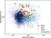 |
Fig. 1. Temperature vs. rise time parameter space for the training dataset, showing the imbalance between TDEs and other classes reported in TNS. |
3.4. Classifier
To solve the issue of our extremely imbalanced dataset, we built a classifier that was able to efficiently generalize the feature behavior of a few positives, thus producing predictions over a feature space that is mostly occupied by negatives. To do this, we used the extreme gradient-boosting algorithm implemented in the XGBOOST10 package (Chen & Guestrin 2016). This method combines the predictions of several weak learners in the form of decision trees to create a stronger learner.
As the dataset is highly imbalanced, we oversampled the positives using the synthetic minority over-sampling technique11 (SMOTE; Chawla et al. 2002). In order to cover the region better with synthetic positives, we applied the oversampling in two steps. We first interpolated the known TDEs up to half of the negatives, and we then interpolated the results to fully balance the dataset. To minimize overfitting, we fixed the hyperparameter defining the maximum depth of individual decision trees (max_depth = 3), forcing them to be shallow. This encourages the splitting of the parameter space into broad regions and thus significantly suppresses overfitting. To optimize the remaining hyperparameters, we used a stratified fivefold cross-validation that maximized the F2 score, defined as
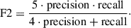 (2)
(2)
This score, in contrast to the standard F1 score, places greater emphasis on recall than on precision, which improves the extrapolation capacities of the classifier despite the heavily imbalanced classes. This favored the reduction of false negatives (TDEs classified as others) at the cost of obtaining more false positives (others classified as TDEs).
Together with the hyperparameter optimization (Table 1), we performed an iterative pruning of features that were not important for the classification results because they might affect the performances on independent datasets and are likely to be highly correlated with other features12. Thus, as detailed in Sect. 3.2, the features fed to the machine-learning model were temperature, rise_time, e_reference_time, and optionally distnr (for the nuclear classifier). We then optimized the hyperparameters by using randomized search over the reasonable range for hyperparameters listed in Table 1 together with stratified fivefold cross-validation to avoid overfitting. We did not optimize the classifier threshold because we observed in our initial tests a very weak dependence of performance scores on it. Thus, we kept the default 0.5 threshold during the optimization and actual use of the classifier.
Hyperparameters of the XGBoost classifier and corresponding final scores, for the nuclear and broad models.
Table 1 shows the final hyperparameter values after optimization.
4. Results
We present the results from the pipeline validation using labels obtained from the literature (Sect. 4.1) as well as a selection of interesting candidates we found during the development of this module (Sect. 4.2).
4.1. Validation
During the hyperparameter optimization, we observed a significant spread of performance scores across the folds at the level of 0.15 for precision and 0.03 for recall. Thus, to assess the classifier performance with optimized parameters when trained on the full dataset, we performed a run of a leave-one-out cross-validation by excluding a single point at a time from the original training set, oversampling, and training on the remaining data. The final scores are listed in Table 1, and the final confusion matrix and relative feature importance are shown in Fig. 2. The very small number of positives in the dataset means that these scores also carry substantial uncertainties, similar to those obtained during the hyperparameter optimization. When the imbalance between the two classes is taken into account, the confusion matrices confirm the success of our initial goal of minimizing the number of false negatives. In both scenarios, the majority of TDEs were identified by the algorithm, 32 (76%) when distnr was available (nuclear classifier), and 31 (74%) otherwise. Despite its minor impact on recall, this additional feature significantly improved precision by enabling the rejection of many contaminants, namely off-nuclear transients such as SNe. The lower panels of the same figure show the dominant importance of this additional feature. The order of importance for the remaining features is maintained when this distance is not available.
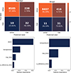 |
Fig. 2. Confusion matrix built using leave-one-out cross-validation (upper panels) and relative feature importance returned by the XGBOOST package (lower panels) for the nuclear (left panels) and broad (right panels) models. The percentages displayed inside the confusion matrices are values normalized on completeness. |
Although the distnr feature aids in filtering out contaminants, it is not essential for a successful classification, as is reflected in its very weak effect on recall, and it might even hinder the identification of rare off-nuclear TDEs. Notably, recent discoveries such as the off-nuclear TDE 2024tvd (Yao et al. 2025) and the TDE-like event AT2024puz (Somalwar et al. 2025a) suggest that relying on this criterion too strongly might be overly restrictive. To balance these considerations, we opted to use both classifiers in parallel, combining their outputs and further investigating promising candidates identified by either classifier.
To evaluate the classifiers on archival data, we applied them to the full dataset described in Sect. 3, which covers observations between Nov 2019 and Feb 2025, including objects not listed in TNS. Figure 3 presents the feature space obtained with the final nuclear model for this full dataset. The proposed candidates (orange dots) occupy the same region of feature space as the known TDEs (circles), while rejected objects (blue dots) lie elsewhere. This shows the usefulness of the chosen features. Interestingly, the only13 known TDE that was not flagged as such in this test run (dark blue circle) is the aforementioned off-nuclear event TDE 2024tvd. This is a direct consequence of its distnr value, which is noticeably higher than that of the other TDEs. This case further justifies also executing the broad model so that the results encompass a wide variety of candidates. Moreover, the case highlights that the model does not simply memorize the training set, but instead generalizes beyond it.
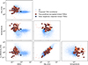 |
Fig. 3. Corner plot showing the complete feature space for the nuclear model on the whole dataset. The small blue dots show the positions of all points in the dataset, and orange dots mark the TDE candidates proposed by the classifier. The orange and dark blue circles show the positions of known TDEs that were accepted and rejected by the classifier, respectively. In contrast to the results shown by the leave-one-out cross-validation in Fig. 2, only one known TDE is not identified by the model in this test because all these TDEs were included in the training set. This outlier is the off-nuclear optical TDE 2024tvd. |
Upon inspection of the reported TDE candidates, we identified several promising TDEs (see Sect. 4.2). This test also provided an indication of the most common impostors encountered in the real live-stream, which slightly differs from those in the TNS sample used during development. In particular, beyond the dominant presence of SNe, as in TNS, the contamination by AGNs is significant because their typical variability might result in rising light-curve segments that resemble the early phases of TDEs. To quantify this contamination, we report numbers from two months of live operation (see Sect. 5.2) instead of quoting statistics from this test, because they correspond to real conditions: out of 438 candidate entries, 94 (21%) were AGNs. This corresponds to 37 unique AGNs among 111 unique objects (33%).
4.2. Some identified candidates
Throughout the different stages of the module development, several interesting transients were identified as potential TDE candidates by analyzing archival data. A detailed analysis of these transients is provided in the companion paper, Quintin et al. (2025). As an illustration, we present a summary of four of these objects here, and their corresponding long-term ZTF light curves are displayed in Fig. 4. The data-release photometry14 used in this Figure was retrieved using the SNAD API (Malanchev et al. 2023). For illustration purposes, we executed the current version of the pipeline (Sect. 5.2) on each alert of these objects and recovered the time at which they would have been first reported if the module had been operational. This is indicated with a vertical dashed line. AT 2023adr, which was found by a previous version of the pipeline, is no longer recovered with the latest version due to stricter preprocessing cuts.
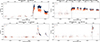 |
Fig. 4. Light curves of four TDE candidates identified from archival data during the development of the module. The full dots represent detections extracted from FINK alerts, and semitransparent dots were extracted from data-release photometry. The vertical dashed black lines mark the times at which these candidates would have been first reported with the current version of the pipeline. |
4.2.1. ZTF19aayijkh/AT2022yhf
This transient15 is hosted by a blue active galaxy located at a photometric redshift of z ∼ 0.56 ± 0.03 (Almeida et al. 2023), classified as a quasar (QSO) by Gaia DR3 (Gaia Collaboration 2023). The host exhibits QSO-like variability on timescales of ∼6 months.
In addition to this variability, a significant brightening event that started on September 2022 was identified by our module as a potential TDE. The flare is characterized by a slow 3- to 4-month rise followed by a steady decay that continues for more than two years after peak brightness (upper left panel of Fig. 4). The event is significantly bluer than in the quiescent state. It is bluest at peak, and little to no reddening is observed during the subsequent decay. The apparent magnitude at the peak of the transient and the host redshift correspond to luminosity values of ∼1044 erg/s in both bands. This luminosity, combined with the observed color evolution, is consistent with a TDE that occurred within the QSO. In addition, data from the Wide-field Infrared Survey Explorer (WISE or NeoWISE, Wright et al. 2010) reveal indications of an associated infrared echo that emerged in May 2025. This corroborates the TDE hypothesis.
4.2.2. ZTF20accxwrk/AT2020ukj
This object16 is a very long-lived transient that has been steadily decaying since its peak in December 2020, as depicted in the upper right panel of Fig. 4. Its host, with a photometric redshift of z ∼ 0.089 (Duncan 2022), was not active beforehand and exhibited a red color (g − r ∼ 1).
The 2020 brightening features a bluer color (reaching g − r ∼ 0.6), which has been reddening steadily since, but has not reached the color of its quiescent state so far. The 2020 brightening features a blue color (differential g − r ∼ −0.25), which has remained constant and thus shown no strong sign of cooling since it has been active. This source exhibits striking similarities to ZTF19acnskyy (Sánchez-Sáez et al. 2024) in terms of timescales, particularly in its exceptionally slow decay compared to the slowest known TDEs. This supports a similar physical interpretation for both objects: either an unusually long-duration TDE, or an AGN in the process of activation.
We acquired two spectra using the 2.5 m telescope from the Caucasian Mountain Observatory (CMO, Shatsky et al. 2020) that support the interpretation of a TDE at z = 0.066 (Russeil et al. 2024b) and not that of a standard AGN. However, the observed luminosity leads to an energy budget that might be too large for the disruption of a single star, favoring the interpretation of a starting AGN. We are currently monitoring this source in X-rays to investigate its multiwavelength behavior.
4.2.3. ZTF22abzajwl/AT2023adr
This object17 presented a flare that started in December 2022 and was first identified as a potential superluminous SN by Perley et al. (2023) and then as a potential TDE by Aleo et al. (2024). A second fainter flare occurred in February 2024, as shown in the lower left panel of Fig. 4. The ePESSTO+ group obtained a spectrum for this object while searching for SNe and located it at z ∼ 0.131 using the clear narrow lines (Shlentsova et al. 2024). The spectrum shows no strong metal lines or very broad emission lines, which might be expected from SNe, and the smoothly evolving light curve tends to exclude some superluminous supernova scenarios, which can display irregular temporal features (see, e.g., Angus et al. 2019; Hosseinzadeh et al. 2022).
Upon identification of this candidate by our module, the TDE-like flares together with the non-SN-like spectrum led us to classify it as a TDE, and in particular, a partially repeated TDE (Llamas Lanza et al. 2024). This discovery adds a new source to the relatively short list of known or candidate repeated TDEs, which include ASASSN-14ko (Payne et al. 2021, 2023), eRASSt J045650.3–203750 (Liu et al. 2023, 2024), AT2018fyk (Wevers et al. 2023), RX J133157.6–324319.7 (Malyali et al. 2023), AT 2020vdq (Somalwar et al. 2025b), and AT 2022dbl (Lin et al. 2024).
4.2.4. ZTF23abjvojy
A brightening event18 that started in October 2023 was flagged by our module as a TDE candidate. The host is a spectroscopically confirmed broadline QSO at z ∼ 0.277 (Almeida et al. 2023), with hints of variability at the quiescent level. The identified flare, however, represents a significant excess from this baseline, as shown in the lower right panel of Fig. 4, and it does not appear to be the typical QSO red-noise variability.
The source rose with a timescale of ∼25 days and became significantly bluer. It decayed in fewer than 200 days, without a significant color change in the decay. Additionally, a clear infrared echo of this transient was found in the NeoWISE light curve. Interestingly, another even brighter flare from this galaxy was visible more than 15 years earlier in data from the Catalina real-time transient survey (CRTS; Drake et al. 2009) that started to rise in January 2008 and slowly decayed over a decade. The timing and luminosity properties of the two brightening episodes are consistent with a TDE or an AGN flare. In particular, the significant asymmetry of the first peak is inconsistent with standard AGN variability. Although it is not possible to conclude on the nature of these bursts without spectral observations, this source is a good candidate to join a small group of repeated TDE-like flares in AGNs, along with AT2019aalc (Milán Veres et al. 2026), AT2021aeuk (Sun et al. 2025), and IRAS F01004-2237 (Sun et al. 2024).
4.3. Early identification performance
Considering that the main objective of this work is to identify candidates as early as possible to enable their follow-up, we assessed how early in their rise we might identify them. To do this, we evaluated each known TDE in our sample using the leave-one-out approach (see Sect. 4.1) to train the nuclear classifier on the whole dataset except for one TDE at a time, and we then applied it for all light-curve segments of the excluded event. This procedure ensured that the resulting models in each iteration were as similar as possible to the final model (presented in Sect. 3.4) while avoiding training on the test object. From this evaluation, we extracted the time of the first alert classified as a rising TDE for each candidate.
Figure 5 shows the time of first identification as a function of the time of maximum flux for each TDE candidate. Both quantities were measured with respect to the first detection within the 100-day window preceding the peak, which itself is defined as the last data point satisfying the rising and not decaying criteria described in Sect. 3.1. Out of the 42 TDEs in the sample, 34 (81%) were correctly classified at least once during their rise, including 4 that were only flagged at the peak (data points on the diagonal). The latter might demand a more rapid follow-up response, depending on their brightness and how fast they decay. Nevertheless, the remaining cases were identified earlier, with the delays predominantly dominated not by the classifier itself, but instead by precedent selection criteria such as the flux availability in both bands. Twelve percent of these TDEs were identified at one-third into their rise, 46% at half the way, and 74% at three-quarters of their rise. This early identification enables a potential monitoring of the remaining rise phase and provides enough time to potentially perform follow-up observations at their peak.
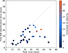 |
Fig. 5. Time of the first alert that led to a TDE candidate identification as a function of the peak-flux time for each known TDE that was correctly classified by our module. Both times are measured with respect to first detection within 100 days prior to the peak. The color scale illustrates the number of detections within this window that culminated in a true-positive classification. |
5. Discussion
5.1. Classifier design choices
Probably the greatest challenge in this work was to conceive a classifier that was able to learn and generalize specific characteristics from the small number of known TDEs available for training. This in turn enabled us to identify unusual or previously unobserved TDE-like events and made the module sensitive to a broader spectrum of behaviors that is consistent with theoretical expectations.
Moreover, we prioritized completeness (recall) over purity (precision). While this increased the likelihood of detecting true TDEs, it also led to a higher rate of false positives and required a subsequent manual vetting step.
In agreement with this philosophy, we decided to loosen certain criteria that might be applied to exclude AGNs, such as stricter cuts on historical activity or removal of AGNs based on catalog cross-matches. This decision was motivated by the possibility of capturing repeated TDEs as well as TDEs that occurred within AGNs, which are theoretically expected to be common, but are challenging to identify observationally in addition to the usual AGN variability. This approach increased the number of false positives because AGNs are one of the main contaminants, but it broadened the range of TDE characteristics that were accessible to this module. In future versions, we plan to refine this approach by incorporating a comparison between the variability observed in the rising phase and the historical baseline activity. This will allow us to distinguish TDE flares better from typical AGN variability, and we will thereby reduce contamination while still preserving completeness. Another example of this completeness-driven philosophy is retaining the broad model, which does not include the distnr feature, even though it is useful in reducing contaminants, in order to remain sensitive to rare off-nuclear TDEs.
5.2. FINK filter implementation
After the classifier was finalized, we proceeded to implement it into the FINK broker19 to enable an automatic processing. In this context, we also aimed for a user-friendly delivery method beyond the classification results, which would allow astronomers to quickly go through potential candidates and thus make informed follow-up decisions. To do this, we implemented a filter within FINK that is applied to the data acquired by the broker after every night of its operation. The filter then selects the candidates and sends them to the dedicated FINK community slack and telegram20 channels for review.
Since the information contained in individual ZTF alerts is limited to 30 days of photometry and access to historical data beyond this is relatively costly, we adjusted the method outlined in Sect. 3.1 for the live filter. We required at least five detections, with at least one point in each band, g and r, and no more than one negative flux in total in these 30 days alone. Moreover, we also required these data points to satisfy the rising and not decaying criteria as described above. Table 2 provides an overview of how many alerts remain after every specific step of this filtering.
Number of alerts at various steps of the processing of the ZTF data stream in 84 nights in January to April 2025.
These steps significantly reduce the number of candidates to approximately 100 per observing night. This number is small enough for a full-scale processing of their historical light curves. From this point on, we applied exactly the same cuts on the number of detections in the fitting, historical, and pre-historical windows (see Fig. A.1) as described in Sect. 3.1. We then extracted features using the detections and upper limits inside the fitting window as described in Sect. 3.2. Finally, we applied quality cuts to these features, as described in Sect. 3.3.
In order to maximize the detection probability, we adopted an approach that accounts to some degree for the statistical uncertainties of the features derived from the light curve during the RAINBOW fitting process. The fitter reports the best-fit values of the parameters together with their covariances. Using this information, multiple feature sets are generated by sampling the distribution of probable parameter values around the best fit in consistency with the fit uncertainties. These sampled feature sets are then passed through the classifier, and a candidate is classified as a potential rising TDE when either the best-fit set or at least 10% of the sampled sets are positively classified as such.
The candidates are then published to the dedicated Slack and Telegram20 channels. For every candidate, the filter constructs a compact card-like representation containing a variety of available information, including the historical light curves reconstructed from the alerts and the latest ZTF data-release photometry (Malanchev et al. 2023), along with the supporting data from TNS and direct links to the FINK science portal and several other online resources that might be useful for a rapid screening of the transient. An example of such a card is shown in Fig. 6 for a light curve that was selected by the module as a candidate. Although it does not correspond to a TDE, we chose this object because it allowed us to clearly illustrate each component of the card, and in particular, because it contains past flares in the pre-historical window (see Sect. 3.1) that are accepted by our module.
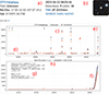 |
Fig. 6. Example information card as produced by the FINK filter and posted to the dedicated Slack channel as a candidate. We chose to show this object, despite not corresponding to a TDE, because it allows to clearly illustrate each of the following elements: (a) information block including the ZTF object identifier, alert time stamp and sky coordinates, along with TNS name and classification when available, and direct links to the FINK object page and several external services that might contain additional useful data about this object; (b) Pan-STARRS cutout image centered at the object position; (c) historical light curve based on data from alerts and (d) latest ZTF data-release photometry; (e) the latest 100-day interval; (f) best fit curve of the data over the last 100 days, plus the probable fits sampled from the covariances of the parameters; (g) values and error bars for the fit parameters and additional features; (h) binary scores from two classifiers for the best fit, and the fraction of probable fits identified as rising TDE candidates. |
5.3. Other classifiers
Comparisons among machine-learning classifiers performances should be interpreted with caution because differences in the datasets, selection criteria, and metadata often prevent a direct equivalence between the analyses. Consequently, classifier results are most meaningful when they are considered within their full methodological context. Nevertheless, we attempted a comparison with the FLEET (Gomez et al. 2023) TDE classifiers to provide a general perspective.
FLEET currently constitutes to the best of our knowledge the only other model that attempts to detect early TDE light curves. We underline, however, that our definitions of early light curves are distinct. While we considered any light curve that was still rising to be early, Gomez et al. (2023) defined it as the first 20 days of data after discovery. A decaying transient that recently appeared might therefore be considered early. Based on this, FLEET was trained using ZTF data, and the sample was limited to sources that lay within the footprint of Pan-STARRS1 (for the host galaxy association). As reported by the authors, from a dataset of 45 TDEs among 4779 transients, it achieved a purity of 50 % and a completeness of 30% for P(TDE) > 0.7. In contrast, our implementation observed a higher completeness for the price of lower purity. For instance, with the distnr metadata, it reached a purity of 12% and a completeness of 76%. We therefore found significantly more TDEs, in particular, events that are challenging to identify with high confidence at early stages. However, this increase is expected to require greater expert involvement to determine which events should be prioritized for follow-up observations. Although it was not optimized for this purpose, the default 0.5 classification threshold can also be manually raised to increase the purity. For example, by only selecting events with a score of 0.99 or greater, the classifier reaches a compromise of ∼40% for both purity and completeness.
5.4. Preparing for the Rubin alert stream
The module we implemented was optimized for the cadence and other properties of the ZTF sky survey. The future plan is to adapt it for the Rubin/LSST data stream, however, which is expected to start producing data in the second half of 2025. While its cadence will be sparser than that of the ZTF (The Rubin Observatory Survey Cadence Optimization Committee SCOC 2025), especially for sky coverage in a single band, the consecutive observations over five to six different bands make it particularly well suited for the feature-extraction approach based on simple parametric multicolor fits such as RAINBOW. Theoretically, we expect a reasonable estimation of the transient rise time and temperature based on a single point in every filter, separated by several days each. This is essentially impossible in a per-band fitting approach. Typical durations of the rising phase of TDEs, along with immediate availability of previous alert data for an entire year and forced photometry at the transient position for at least 30 days prior to the first detection directly in the alert packets, will allow us to acquire enough data points for the fit. Thus, we expect that even without additional support from the local database, we will have enough data points for an accurate estimation of the transient physical parameters, and we will thus be able to classify it rapidly.
The enhanced detection capabilities of Rubin and the expected LSST alert rate of approximately 10 million per night means that the number of candidates reported by the module is expected to increase substantially. To maintain a manageable number of candidates per night for manual vetting, the module might need to be adapted to operate in a more restrictive regime, which likely reduces the number of false positives at the cost of a lower completeness. Among other measures, applying stricter cuts on past variability (see Sect. 5.1) will substantially reduce the number of false positives from AGNs and newly discovered variable stars that are not flagged by existing catalogs.
To train the classifier for Rubin data, it might initially be necessary to rely on simulated datasets, such as those provided by ELAsTiCC (Narayan & ELAsTiCC Team 2023). As the survey progresses and a sufficient sample of TDEs is identified by Rubin, the model can be retrained using real observational data. This retraining might also benefit from active learning strategies (e.g., Leoni et al. 2022; Möller et al. 2025) to efficiently incorporate new labeled examples.
6. Conclusions
We presented the development of an early TDE identification module for the FINK broker using optical photometry data from the ZTF. The pipeline involves several filtering steps to discard irrelevant alerts and the application of the RAINBOW multiband fitting framework to rising light curves in order to extract a set of physically meaningful features. These features were then used as input to a machine-learning classifier that was trained to distinguish TDEs from other types of rising transients, such as SNe, prior to their peak brightness.
The training dataset consisted of 8865 entries that passed all preceding cuts, and only 42 were labeled as TDEs. Two variants of the classifier were employed: the broad classifier, which only used three parameters extracted from the fit, and the nuclear classifier, which also included an additional contextual feature, the angular distance to the closest object in the ZTF reference catalog, distnr. This value generally improved the model performance because it helps to distinguish nuclear transients such as most TDEs from off-nuclear events such as SNe. However, because this quantity might not always indicate the distance to the real host and might limit the possibility of identifying off-nuclear TDEs, the two models are run in parallel at the current stage.
The nuclear classifier achieves a recall of 76% and a precision of 12%. This performance reflects a design choice: We prioritized completeness (i.e., high recall) over purity to ensure that we captured a broad set of candidates, even at the cost of more false positives. As a result, manual vetting by experts remains essential to filter down to the most promising sources for multiwavelength follow-up, such as spectroscopy and X-ray observations. The module is executed in FINK after each night of ZTF observations and reports a list of candidates (currently, one to two per night) to dedicated slack and telegram channels for visual inspection.
Importantly, the classification is based exclusively on the rising part of a the candidate light curve. The goal of this design choice was to enable timely follow-up for the most promising candidates. This goal was successfully achieved because at least half of the known TDEs identified by our module were flagged before they reached 52% of their rising phase. This early identification provides ample time for coordinating the monitoring of the remaining rise and further follow-up observations around peak brightness. One of our goals for future development is to increase the performance in this early identification capability.
Throughout the module development, several interesting transients were identified among the reported candidates when we tested it on archival ZTF data. While they are likely not all TDEs, many are scientifically interesting and worthwhile an investigation. Sect. 4 briefly presents four of these sources, and a more detailed description of these and other transients is presented in the companion article, Quintin et al. (2025).
Despite the considerable effort devoted to the study of TDEs, we still cannot fully satisfactorily describe their physical nature. The advent of large-scale sky surveys such as ZTF and soon LSST enables a statistical characterization of these events. This information can be used to fill the gaps of theoretical knowledge with observational data and serve as a starting point for further development. Nevertheless, real-time coordination between the many players involved in the data-taking and analysis process is crucial to ensure an optimized science output from these rich datasets. We showed one possible approach to ensure an optimal exploitation of photometric surveys to enable TDE science. Subsequent work will focus on the analysis of a larger sample of candidates, on the refinement of the preprocessing steps, and on modifications for operation under Rubin.
Acknowledgments
We thank Hui Yang for helpful comments on the draft. EQ acknowledges support from the European Space Agency, through the Internal Research Fellowship programme. EQ acknowledges funding from the European Union’s Horizon 2020 research and innovation programme under grant agreement number 101004168, the XMM2ATHENA project (Webb et al. 2023). MVP contribution was carried out under the state assignment of Lomonosov Moscow State University. ER was Funded by the European Union (ERC, project number 101042299, TransPIre). Views and opinions expressed are however those of the author(s) only and do not necessarily reflect those of the European Union or the European Research Council Executive Agency. Neither the European Union nor the granting authority can be held responsible for them. This work was developed within the FINK community and made use of the FINK community broker resources. FINK is supported by LSST-France and CNRS/IN2P3. AM is supported by the Australian Research Council Discovery Early Research Award (DE230100055). Parts of this research were conducted by the Australian Research Council Centre of Excellence for Gravitational Wave Discovery (OzGrav), through project number CE230100016. This research has made use of the SIMBAD database, operated at CDS, Strasbourg, France. This work was co-funded by the European Union and supported by the Czech Ministry of Education, Youth and Sports (Project No. CZ.02.01.01/00/22_008/0004632 – FORTE).
References
- Aleo, P., Engel, A., Narayan, G., et al. 2024, ApJ, 974, 172 [Google Scholar]
- Almeida, A., Anderson, S. F., Argudo-Fernández, M., et al. 2023, ApJS, 267, 44 [NASA ADS] [CrossRef] [Google Scholar]
- Angus, C. R., Smith, M., Sullivan, M., et al. 2019, MNRAS, 487, 2215 [NASA ADS] [CrossRef] [Google Scholar]
- Bade, N., Komossa, S., & Dahlem, M. 1996, A&A, 309, L35 [NASA ADS] [Google Scholar]
- Ban, M., Voloshyn, P., Adomavicienė, R., et al. 2025, A&A, 697, A57 [NASA ADS] [CrossRef] [EDP Sciences] [Google Scholar]
- Bellm, E. 2014, in The Third Hot-wiring the Transient Universe Workshop, 27 [Google Scholar]
- Bellm, E. C., Kulkarni, S. R., Graham, M. J., et al. 2019, PASP, 131, 018002 [Google Scholar]
- Biswas, B., Ishida, E., Peloton, J., et al. 2023, A&A, 677, A77 [NASA ADS] [CrossRef] [EDP Sciences] [Google Scholar]
- Bloom, J. S., Giannios, D., Metzger, B. D., et al. 2011, Science, 333, 203 [CrossRef] [PubMed] [Google Scholar]
- Chawla, N. V., Bowyer, K. W., Hall, L. O., & Kegelmeyer, W. P. 2002, J. Artif. Intell. Res., 16, 321 [CrossRef] [Google Scholar]
- Chen, T., & Guestrin, C. 2016, in Proceedings of the 22nd ACM SIGKDD International Conference on Knowledge Discovery and Data Mining, KDD ’16 (New York, NY, USA: Association for Computing Machinery), 785 [Google Scholar]
- Dai, L., McKinney, J. C., Roth, N., Ramirez-Ruiz, E., & Miller, M. C. 2018, ApJ, 859, L20 [Google Scholar]
- Drake, A., Djorgovski, S., Mahabal, A., et al. 2009, ApJ, 696, 870 [NASA ADS] [CrossRef] [Google Scholar]
- Duncan, K. J. 2022, MNRAS, 512, 3662 [NASA ADS] [CrossRef] [Google Scholar]
- Förster, F., Cabrera-Vives, G., Castillo-Navarrete, E., et al. 2021, AJ, 161, 242 [CrossRef] [Google Scholar]
- Fraga, B. M. O., Bom, C. R., Santos, A., et al. 2024, A&A, 692, A208 [NASA ADS] [CrossRef] [EDP Sciences] [Google Scholar]
- Gaia Collaboration (Bailer-Jones, C. A. L., et al.) 2023, A&A, 674, A41 [NASA ADS] [CrossRef] [EDP Sciences] [Google Scholar]
- Gezari, S. 2021, ARA&A, 59, 21 [NASA ADS] [CrossRef] [Google Scholar]
- Gomez, S., Villar, V. A., Berger, E., et al. 2023, ApJ, 949, 113 [Google Scholar]
- Gordon, K. D. 2024, J. Open Source Softw., 9, 7023 [NASA ADS] [CrossRef] [Google Scholar]
- Gordon, K. D., Clayton, G. C., Decleir, M., et al. 2023, ApJ, 950, 86 [CrossRef] [Google Scholar]
- Guillochon, J., & Ramirez-Ruiz, E. 2013, ApJ, 767, 25 [NASA ADS] [CrossRef] [Google Scholar]
- Guolo, M., Gezari, S., Yao, Y., et al. 2024, ApJ, 966, 160 [NASA ADS] [CrossRef] [Google Scholar]
- Hammerstein, E., van Velzen, S., Gezari, S., et al. 2022, ApJ, 942, 9 [Google Scholar]
- Hills, J. G. 1975, Nature, 254, 295 [Google Scholar]
- Hills, J. G. 1988, Nature, 331, 687 [Google Scholar]
- Hosseinzadeh, G., Berger, E., Metzger, B. D., et al. 2022, ApJ, 933, 14 [NASA ADS] [CrossRef] [Google Scholar]
- Hung, T., Gezari, S., Blagorodnova, N., et al. 2017, ApJ, 842, 29 [NASA ADS] [CrossRef] [Google Scholar]
- Ivezić, Ž., Kahn, S. M., Tyson, J. A., et al. 2019, ApJ, 873, 111 [Google Scholar]
- Kessler, R., Bernstein, J. P., Cinabro, D., et al. 2009, PASP, 121, 1028 [Google Scholar]
- Langis, D. A., Liodakis, I., Koljonen, K. I. I., et al. 2025, arXiv e-prints [arXiv:2506.05476] [Google Scholar]
- Le Montagner, R., Peloton, J., Carry, B., et al. 2023, A&A, 680, A17 [NASA ADS] [CrossRef] [EDP Sciences] [Google Scholar]
- Leoni, M., Ishida, E. E., Peloton, J., & Möller, A. 2022, A&A, 663, A13 [NASA ADS] [CrossRef] [EDP Sciences] [Google Scholar]
- Lin, Z., Jiang, N., Wang, T., et al. 2024, ApJ, 971, L26 [NASA ADS] [CrossRef] [Google Scholar]
- Liu, Z., Malyali, A., Krumpe, M., et al. 2023, A&A, 669, A75 [NASA ADS] [CrossRef] [EDP Sciences] [Google Scholar]
- Liu, Z., Ryu, T., Goodwin, A., et al. 2024, A&A, 683, L13 [NASA ADS] [CrossRef] [EDP Sciences] [Google Scholar]
- Llamas Lanza, M., Quintin, E., Russeil, E., et al. 2024, TNSAN, 178, 1 [Google Scholar]
- Mahabal, A., Rebbapragada, U., Walters, R., et al. 2019, PASP, 131, 038002 [NASA ADS] [CrossRef] [Google Scholar]
- Malanchev, K., Kornilov, M. V., Pruzhinskaya, M. V., et al. 2023, PASP, 135, 024503 [CrossRef] [Google Scholar]
- Malyali, A., Liu, Z., Rau, A., et al. 2023, MNRAS, 520, 3549 [NASA ADS] [CrossRef] [Google Scholar]
- Masson, M., & Bregeon, J. 2024, arXiv e-prints [arXiv:2412.05061] [Google Scholar]
- Masterson, M., De, K., Panagiotou, C., et al. 2024, ApJ, 961, 211 [NASA ADS] [CrossRef] [Google Scholar]
- Matheson, T., Stubens, C., Wolf, N., et al. 2021, AJ, 161, 107 [NASA ADS] [CrossRef] [Google Scholar]
- Milán Veres, P., Franckowiak, A., van Velzen, S., et al. 2026, A&A, in press, https://doi.org/10.1051/0004-6361/202452051 [Google Scholar]
- Möller, A., & de Boissière, T. 2020, MNRAS, 491, 4277 [CrossRef] [Google Scholar]
- Möller, A., Peloton, J., Ishida, E., et al. 2021, MNRAS, 501, 3272 [CrossRef] [Google Scholar]
- Möller, A., Ishida, E., Peloton, J., et al. 2025, PASA, 42, e057 [Google Scholar]
- Narayan, G.& ELAsTiCC Team 2023, AAS Meet. Abstr., 241, 117.01 [Google Scholar]
- Nordin, J., Brinnel, V., van Santen, J., et al. 2019, A&A, 631, A147 [NASA ADS] [CrossRef] [EDP Sciences] [Google Scholar]
- Pavez-Herrera, M., Sánchez-Sáez, P., Hernández-García, L., et al. 2025, A&A, 696, A153 [NASA ADS] [CrossRef] [EDP Sciences] [Google Scholar]
- Payne, A. V., Shappee, B. J., Hinkle, J. T., et al. 2021, ApJ, 910, 125 [NASA ADS] [CrossRef] [Google Scholar]
- Payne, A. V., Auchettl, K., Shappee, B. J., et al. 2023, ApJ, 951, 134 [NASA ADS] [CrossRef] [Google Scholar]
- Perley, D., Lunnan, R., Wise, J., et al. 2023, TNSAN, 26, 1 [Google Scholar]
- Pessi, P. J., Durgesh, R., Nakazono, L., et al. 2024, A&A, 691, A181 [NASA ADS] [CrossRef] [EDP Sciences] [Google Scholar]
- Pfeffermann, E., Briel, U., Hippmann, H., et al. 1986, in Soft X-ray Optics and Technology (Spie), 733, 519 [Google Scholar]
- Quintin, E., Russeil, E., Llamas Lanza, M., et al. 2025, A&A, submitted [arXiv:2511.19016] [Google Scholar]
- Rees, M. J. 1988, Nature, 333, 523 [Google Scholar]
- Russeil, E., Malanchev, K. L., Aleo, P. D., et al. 2024a, A&A, 683, A251 [NASA ADS] [CrossRef] [EDP Sciences] [Google Scholar]
- Russeil, E., Quintin, E., Llamas Lanza, M., et al. 2024b, TNS Classif. Rep., 2024-5006, 1 [Google Scholar]
- Sánchez-Sáez, P., Reyes, I., Valenzuela, C., et al. 2021, AJ, 161, 141 [CrossRef] [Google Scholar]
- Sánchez-Sáez, P., Hernández-García, L., Bernal, S., et al. 2024, A&A, 688, A157 [NASA ADS] [CrossRef] [EDP Sciences] [Google Scholar]
- Saxton, C. J., Perets, H. B., & Baskin, A. 2018, MNRAS, 474, 3307 [NASA ADS] [CrossRef] [Google Scholar]
- Schlegel, D. J., Finkbeiner, D. P., & Davis, M. 1998, ApJ, 500, 525 [Google Scholar]
- The Rubin Observatory Survey Cadence Optimization Committee SCOC 2025, Survey Cadence Optimization Committee’s Phase 3 Recommendations, Tech. Rep. PSTN-056 [Google Scholar]
- Shatsky, N., Belinski, A., Dodin, A., et al. 2020, arXiv e-prints [arXiv:2010.10850] [Google Scholar]
- Sheng, X., Nicholl, M., Smith, K. W., et al. 2024, MNRAS, 531, 2474 [Google Scholar]
- Shlentsova, A., Hoof, A., Dalen, J., et al. 2024, TNSAN, 98, 1 [Google Scholar]
- Smith, K. W., Williams, R. D., Young, D. R., et al. 2019, Res. Notes AAS, 3, 26 [Google Scholar]
- Somalwar, J. J., Ravi, V., Margutti, R., et al. 2025a, arXiv e-prints [arXiv:2505.11597] [Google Scholar]
- Somalwar, J. J., Ravi, V., Yao, Y., et al. 2025b, ApJ, 985, 175 [Google Scholar]
- Stein, R., Mahabal, A., Reusch, S., et al. 2024, ApJ, 965, L14 [Google Scholar]
- Sun, L., Jiang, N., Dou, L., et al. 2024, A&A, 692, A262 [NASA ADS] [CrossRef] [EDP Sciences] [Google Scholar]
- Sun, J., Guo, H., Gu, M., et al. 2025, ApJ, 982, 150 [Google Scholar]
- van Velzen, S., Holoien, T. W.-S., Onori, F., Hung, T., & Arcavi, I. 2020, Space Sci. Rev., 216, 1 [CrossRef] [Google Scholar]
- Webb, N. A., Carrera, F. J., Schwope, A., et al. 2023, Astron. Nachr., 344, e20220102 [Google Scholar]
- Wenger, M., Ochsenbein, F., Egret, D., et al. 2000, A&AS, 143, 9 [NASA ADS] [CrossRef] [EDP Sciences] [Google Scholar]
- Wevers, T., Coughlin, E., Pasham, D., et al. 2023, ApJ, 942, L33 [NASA ADS] [CrossRef] [Google Scholar]
- Wright, E. L., Eisenhardt, P. R., Mainzer, A. K., et al. 2010, AJ, 140, 1868 [Google Scholar]
- Yao, Y., Ravi, V., Gezari, S., et al. 2023, ApJ, 955, L6 [NASA ADS] [CrossRef] [Google Scholar]
- Yao, Y., Chornock, R., Ward, C., et al. 2025, ApJ, 985, L48 [Google Scholar]
- Yuan, W., Zhang, C., Feng, H., et al. 2015, arXiv e-prints [arXiv:1506.07735] [Google Scholar]
Other brokers dedicated to Rubin processing are ALeRCE (Förster et al. 2021), AMPEL (Nordin et al. 2019), Antares (Matheson et al. 2021), Babamul, Lasair (Smith et al. 2019) and Pitt-Google.
The real-bogus score (Mahabal et al. 2019) must be above 0.55, and there should be no prior-tagged bad pixels in a 5 × 5 pixel stamp around the alert position.
These rise time values correspond to τrise in Eq. (1), which is shorter by definition than the full duration of the observed rising time. This explains the comparatively low values.
XGBoost: eXtreme Gradient Boosting library, https://xgboost.readthedocs.io/en/release_3.0.0/
We used SMOTE implementation from IMBALANCED-LEARN package, https://github.com/scikit-learn-contrib/imbalanced-learn
The bolometric definition of the amplitude in RAINBOW, for instance (see Eq. (1)), makes it highly correlated with the temperature given the measurements in a fixed spectral band. This reduces its effectiveness for the classification.
Most known TDEs were identified as they were all used to train the model.
Data-release photometry refers to ZTF detections available in public data releases, but not necessarily triggered as real-time alerts.
The code is publicly available at https://github.com/astrolabsoftware/fink-filters/tree/master/fink_filters/ztf/filter_early_tde_candidates
Appendix A: Illustration of light curve window selection and fit
This appendix aims to show a visual example of the different light curve windows defined in Sect. 3.1 (fitting, historical and pre-historical), together with the corresponding RAINBOW fit described in Sect. 3.2. To ease the visualization, we selected an object classified as Seyfert 1 exhibiting a rising segment with clear preceding activity.
The upper panel of Fig. A.1 shows the full light curve with alerts represented by full circles and data-release photometry by translucent dots. Black vertical dashed lines mark the 100-day rising interval for fitting, the hatched region marks the immediate historical 100-day window prior to that, used to constrain ongoing continuous activity, and everything prior to that is the pre-historical period used to additionally restrict long-term behavior. The window selection shown here corresponds to the last alert that passed the criteria presented in Sect. 3.1 (posterior alerts are significantly decaying). Note in order to allow for repeated TDE flares, pre-historical activity is allowed, if there is at most one point with negative flux.
The lower panel of Fig. A.1 shows the data points within the fitting window together with the results of the corresponding RAINBOW fit. The best-fit parameter values and corresponding uncertainties are annotated on the figure for reference.
 |
Fig. A.1. Illustration on the window selection and feature extraction processes. The upper panel shows the complete light curve extracted from the alerts (full circles) and from data-release photometry (translucent dots) with the fitting, historical and pre-historical windows described in Sect. 3.1 indicated for context. Lower panel displays the data points within the 100-day fitting window, along with the corresponding RAINBOW fit output (Sect. 3.2). The dashed lines correspond to the best fit parameter values, while the translucent ones show the scatter of models with parameters sampled around the best fit according to the estimated covariances. The in-figure annotation lists the values of the best fit parameters along with their uncertainties, as well as some additional features such as distnr. |
All Tables
Hyperparameters of the XGBoost classifier and corresponding final scores, for the nuclear and broad models.
Number of alerts at various steps of the processing of the ZTF data stream in 84 nights in January to April 2025.
All Figures
|
Fig. 1. Temperature vs. rise time parameter space for the training dataset, showing the imbalance between TDEs and other classes reported in TNS. |
| In the text | |
|
Fig. 2. Confusion matrix built using leave-one-out cross-validation (upper panels) and relative feature importance returned by the XGBOOST package (lower panels) for the nuclear (left panels) and broad (right panels) models. The percentages displayed inside the confusion matrices are values normalized on completeness. |
| In the text | |
|
Fig. 3. Corner plot showing the complete feature space for the nuclear model on the whole dataset. The small blue dots show the positions of all points in the dataset, and orange dots mark the TDE candidates proposed by the classifier. The orange and dark blue circles show the positions of known TDEs that were accepted and rejected by the classifier, respectively. In contrast to the results shown by the leave-one-out cross-validation in Fig. 2, only one known TDE is not identified by the model in this test because all these TDEs were included in the training set. This outlier is the off-nuclear optical TDE 2024tvd. |
| In the text | |
|
Fig. 4. Light curves of four TDE candidates identified from archival data during the development of the module. The full dots represent detections extracted from FINK alerts, and semitransparent dots were extracted from data-release photometry. The vertical dashed black lines mark the times at which these candidates would have been first reported with the current version of the pipeline. |
| In the text | |
|
Fig. 5. Time of the first alert that led to a TDE candidate identification as a function of the peak-flux time for each known TDE that was correctly classified by our module. Both times are measured with respect to first detection within 100 days prior to the peak. The color scale illustrates the number of detections within this window that culminated in a true-positive classification. |
| In the text | |
|
Fig. 6. Example information card as produced by the FINK filter and posted to the dedicated Slack channel as a candidate. We chose to show this object, despite not corresponding to a TDE, because it allows to clearly illustrate each of the following elements: (a) information block including the ZTF object identifier, alert time stamp and sky coordinates, along with TNS name and classification when available, and direct links to the FINK object page and several external services that might contain additional useful data about this object; (b) Pan-STARRS cutout image centered at the object position; (c) historical light curve based on data from alerts and (d) latest ZTF data-release photometry; (e) the latest 100-day interval; (f) best fit curve of the data over the last 100 days, plus the probable fits sampled from the covariances of the parameters; (g) values and error bars for the fit parameters and additional features; (h) binary scores from two classifiers for the best fit, and the fraction of probable fits identified as rising TDE candidates. |
| In the text | |
|
Fig. A.1. Illustration on the window selection and feature extraction processes. The upper panel shows the complete light curve extracted from the alerts (full circles) and from data-release photometry (translucent dots) with the fitting, historical and pre-historical windows described in Sect. 3.1 indicated for context. Lower panel displays the data points within the 100-day fitting window, along with the corresponding RAINBOW fit output (Sect. 3.2). The dashed lines correspond to the best fit parameter values, while the translucent ones show the scatter of models with parameters sampled around the best fit according to the estimated covariances. The in-figure annotation lists the values of the best fit parameters along with their uncertainties, as well as some additional features such as distnr. |
| In the text | |
Current usage metrics show cumulative count of Article Views (full-text article views including HTML views, PDF and ePub downloads, according to the available data) and Abstracts Views on Vision4Press platform.
Data correspond to usage on the plateform after 2015. The current usage metrics is available 48-96 hours after online publication and is updated daily on week days.
Initial download of the metrics may take a while.