| Issue |
A&A
Volume 705, January 2026
|
|
|---|---|---|
| Article Number | A152 | |
| Number of page(s) | 14 | |
| Section | Cosmology (including clusters of galaxies) | |
| DOI | https://doi.org/10.1051/0004-6361/202556629 | |
| Published online | 16 January 2026 | |
Measuring the dark matter self-interaction cross-section with deep compact clustering for robust machine learning inference
1
Laboratoire d’Astrophysique, EPFL, Observatoire de Sauverny 1290 Versoix, Switzerland
2
Department of Computing Sciences, Bocconi University Milano, Italy
★ Corresponding author: This email address is being protected from spambots. You need JavaScript enabled to view it.
Received:
28
July
2025
Accepted:
28
November
2025
Abstract
We have developed a machine learning algorithm capable of detecting ‘out-of-domain data’ for trustworthy cosmological inference. By using data from two separate suites of cosmological simulations, we show that our algorithm is able to determine whether ‘observed’ data is consistent with its training domain, returning confidence estimates as well as accurate parameter estimations. We applied our algorithm to 2D images of galaxy clusters from the BAHAMAS-SIDM and DARKSKIES simulations with the aim of measuring the self-interaction cross-section of dark matter. Through deep compact clustering, we constructed an informative latent space where galaxy clusters were mapped to the latent space forming ‘latent clusters’ for each simulation, with the location of the latent cluster corresponding to the macroscopic parameters, such as the cross-section, σDM/m. We then passed through mock observations, where the location of the observed latent cluster informed us of which properties are shared with the training data. If the observed latent cluster shares no similarities with latent clusters from the known simulations, we can conclude that our simulations do not represent the observations and discard any parameter estimations. This thus provides us with a method of measuring measure machine learning confidence. This method serves as a blueprint for transparent and robust inference that is in demand in scientific machine learning.
Key words: methods: data analysis / galaxies: clusters: general / dark matter
© The Authors 2026
 Open Access article, published by EDP Sciences, under the terms of the Creative Commons Attribution License (https://creativecommons.org/licenses/by/4.0), which permits unrestricted use, distribution, and reproduction in any medium, provided the original work is properly cited.
This article is published in open access under the Subscribe to Open model. This email address is being protected from spambots. You need JavaScript enabled to view it. to support open access publication.
1. Introduction
Evidence of the existence of some unobservable ‘dark matter’ (DM) that dominates 85% of the Universe’s matter content has been building since the early 20th century (Zwicky 2009; Rubin et al. 1978, 1980), and has now become a central pillar of the cosmological model (Planck Collaboration VI 2020). Particle physics models generally explain this mysterious matter as a massive particle that interacts only gravitationally with baryonic matter, with observations and simulations favouring a ‘cold and collisionless dark matter model’ (hereafter referred to as CDM) (Copi et al. 1995; Burles & Tytler 1998; Peacock et al. 2001; Clowe et al. 2006; Planck Collaboration VI 2020; White et al. 1987; Davis et al. 1982).
Despite its success, CDM has faced a number of challenges in recent years. In particular, a lack of diversity in the rotation curves of dark matter-dominated dwarf galaxies has ignited new models of non-standard DM (Oman et al. 2015). In general, astronomical DM can be modified in two ways: it can be relativistic at early times such that it free-streams out of small halos suppressing power on small scales in a top-down formation mechanism (Bode et al. 2001), or a self-interaction in the dark sector that can create repulsive pressures, reducing large density gradients (Spergel & Steinhardt 2000). Both have been extensively studied in the last decade; however, in this work we focus on self-interacting dark matter (SIDM) as a plausible model for DM.
Self-interacting dark matter was first proposed by Carlson et al. (1992) as a warm alternative to hot dark matter and CDM; however, de Laix et al. (1995) concluded that this version of SIDM could not match observations. Spergel & Steinhardt (2000) proposed an alternate version of SIDM that extends CDM through non-dissipative self-interactions to solve small-scale problems. Primarily (at the time) this aimed to solve the missing satellites and core-cusp problems. Dark matter self-interactions are often assumed to be elastic with a mean free path of the order of 1 kpc to 1 Mpc with either a velocity-independent or dependent cross-section in the range of σDM/m = 0.1 − 450 cm2g−1. Indeed it is possible to constrain SIDM in both dwarf galaxies and galaxy clusters where the mass to light ratios are extremely high. However, in this work we focus on the high-mass end, where SIDM can introduce perturbations to the mass distribution that can be probed by gravitational lensing.
Current methods of measuring the self-interaction cross-section in galaxy clusters vary depending on the dynamical state of the cluster. Most approaches rely on measuring either the shape of the halo (since SIDM makes halos more spherical) (Peter et al. 2013) or the density profile of the cluster, either directly through gravitational lensing (Sagunski et al. 2021) or indirectly through displacements between the brightest cluster galaxy (BCG) and the lensing-inferred centre of the DM distribution in merging and relaxed galaxy clusters (Kim et al. 2017; Sirks et al. 2024; Harvey et al. 2019). Despite efforts to constrain SIDM using lensing, progress is limited, leading us to explore the use of machine learning to efficiently extract DM information without the use of summary statistics in galaxy clusters, mitigating the following hurdles:
-
Observables are often degenerate with simulation nuisance parameters including feedback from the central active galactic nucleus (AGN) or the softening length of the simulation (Roche et al. 2024).
-
Detailed strong lensing analyses of clusters that attempt to model many hundreds of multiply lensed systems are slow and often assume central density profiles derived from simulations of CDM (Johnson et al. 2014; Richard et al. 2014). In the advent of stage IV telescopes such as Euclid (Laureijs et al. 2012) and the Vera Rubin Telescope (Ivezić et al. 2019), we anticipate a significant increase in the number of galaxy cluster observations.
-
Parametric gravitational lensing models fitted to data to estimate the shape or position of halos often assume that the halos are smooth and elliptically symmetric, which can result in important information loss.
Machine learning (ML) offers a model-agnostic approach to feature learning and parameter estimation without relying on summary statistics or specific models (Hoyle 2016; Huertas-Company & Lanusse 2023). A neural network (NN) is a sub-type of ML that is composed of series of simple linear transforms combined with non-linear functions parametrised by weights optimised through an objective, the loss function, and gradient decent algorithms to create a universal function approximator (see Sen et al. 2022 for a review). The flexible nature of ML enables it to solve a broad host of problems (e.g. Euclid Collaboration 2024), leading it to become commonplace in astronomy. However, ML remains a ‘black-box’ in nature, with limited interpretability and transparency. This is particularly pertinent when we are attempting to train algorithms on complex simulations and then apply to noisy data to make inferences on the nature of dark matter.
Recently, a study applied deep learning to SIDM, training their architecture on images of galaxy clusters to classify different models of SIDM from collisionless CDM with different levels of astrophysical feedback (Harvey 2024, hereafter H24). They trained using the BAHAMAS-SIDM hydro-dynamic simulations (McCarthy et al. 2017; Robertson et al. 2019), adapting the Inception-v4 convolutional NN architecture from Szegedy et al. (2017) and Merten et al. (2019) achieving ∼80% accuracy in classifying the models CDM and SIDM with σDM/m = 0.1 cm2 g−1 and σDM/m = 1.0 cm2 g−1. The performance of the NN was also tested on an unseen SIDM model with σDM/m = 0.3 cm2 g−1; however, since this study used a classification architecture, the NN’s output can only estimate the probabilities for the previous three models. Therefore, to obtain an estimate for σDM/m, they treated the output as a poorly sampled probability distribution function (PDF) with the expectation of the probability distribution of n clusters being the estimated cross-section for the model. The accuracy for a single galaxy cluster was δσDM/m = 0.1 cm2 g−1 with the uncertainty decreasing by  for n galaxy clusters.
A key limitation shared by H24 and other cosmological deep learning methods is that the hydro-simulations are fine-tuned; therefore, any algorithm trained on that data will inherently be non-general. Hence, when applied to a new set of simulations or observations that do not reflect the simulated data, it will be forced to extrapolate, returning unreliable estimations. In most areas of scientific research, we use empirical systematic checks to verify that the model fits the data well; for example, goodness of fit statistics. However, ML does not have such a check. In particular, it has no way of informing the user that the test data is related in any way to the training data, returning inferences with little insight into how well it fits the data.
In this paper, we extend the work of H24 in two key directions. First, we design a regression-based architecture to estimate an arbitrary cross-section along with an associated probability distribution to capture the uncertainty of the estimation. Second, we introduce an interpretable latent space, a low-dimensional representation of the data, to address the confidently wrong problem of NNs, particularly in classification, where any input will be assigned a probability for each class without the option to say that the input is outside the training domain. Given that we utilise a variety of simulation suites, we do not follow a single cosmology, and explicitly state throughout which one is assumed.
2. Data
A key aim of this paper is to develop an algorithm that can return a confidence measure for its estimations based on the known data in the learned latent space. As such we require independent datasets that have differing choices of hydro-parameters, particle mass resolution (and subsequent softening), cosmologies, and box sizes. This led us to adopt two key suites of simulations, with an overview of the datasets shown in Table 1.
-
BAHAMAS-SIDM (McCarthy et al. 2017; Robertson et al. 2019), as used by H24: A cosmological box with a side length of 400 Mpc h−1, 2 × 10243 particles and WMAP 9-year cosmology (Hinshaw et al. 2013), where the particle mass is 5.5 × 10⁹ M⊙ for DM, and 1.1 × 10⁹ M⊙ for baryons. For redshifts z > 3, the Plummer-equivalent gravitational softening length is fixed in comoving coordinates; while below z < 3 it is 5.7 pkpc. The dataset comprises three CDM models with varying levels of baryonic feedback, alongside three SIDM models with different cross-sections: BAHAMAS-0w (weak baryonic feedback), BAHAMAS-0 (fiducial CDM), BAHAMAS-0s (strong baryonic feedback), BAHAMAS-0.1 (σDM/m = 0.1 cm2g−1), BAHAMAS-0.3 (σDM/m = 0.3 cm2g−1), and BAHAMAS-1 (σDM/m = 1 cm2g−1). Each model analyses the 300 most massive galaxy clusters across four redshift snapshots at z = 0, 0.125, 0.25, and 0.375. Each snapshot includes three projections, one along each principal axis, resulting in 3600 simulated observations per simulation.
Table 1.Datasets used to train and test in this work.
-
DARKSKIES: A suite of SIDM zoom-in simulations (Harvey et al. 2025). This suite of simulations mimics the initial box size of BAHAMAS by first generating an initial low-resolution DM only box of size 400 Mpc h−1 with 2563 particles and Planck cosmology (Planck Collaboration VI 2020) to find the most massive DM halos. It then re-simulates a higher resolution zoom-in region with baryons. The zoom-in regions are cut at 5 virial radii in length. The simulations are super-sampled such that the DM particle mass is much lower than the gas mass: mdm = 6.8 × 10⁷ M⊙ and mg = 8.2 × 10⁸ M⊙ for DM and baryons, respectively. The Plummer-equivalent comoving softening length is 2.28 pkpc. The dataset comprises one CDM and five SIDM models, we use the CDM and two SIDM simulations: DARKSKIES-0, DARKSKIES-0.1 (σDM/m = 0.1 cm2g−1), and DARKSKIES-0.2 (σDM/m = 0.2 cm2g−1). Each model simulates the 100 most massive galaxy clusters across four redshift snapshots at z = 0, 0.125, 0.25, and 0.375. Each snapshot includes three projections, one along each principal axis, resulting in a total of 1,200 simulated observations per simulation.
In all cases the input data consists of total mass maps that include contributions from DM, stellar, gas and black hole particles, as this can be obtained from weak lensing observations of galaxy clusters and is the most useful for distinguishing between DM models. To generate these we simply sumed all the mass within each pixel to a projected depth of 10 Mpc. This is sufficient to account for all correlated line-of-sight structure. We can also use the X-ray emission as an additional channel in the input to provide more information about the gas of the galaxy clusters as this will be useful in identifying differences in baryonic feedback; however, due to differences in how these maps are created between different suites of simulations, we found that this induces biases (whereas total mass maps is just the summed projected mass). Therefore, to reduce modelling uncertainties, we focus solely on total mass maps. Each map was binned to δx = 20 pkpc, and out to 2 Mpc, resulting in an image dimensions of 100 × 100.
Both the BAHAMAS and the DARKSKIES simulations invoke elastic, velocity-independent cross-sections that have isotropic scatterings. To first approximation, both use a similar probabilistic scattering mechanism where they calculate the local density including the number of nearest neighbours and calculate the probability of scattering. To ensure that the validity of the scattering equations hold, the time-steps of each simulation are reduced such that we expect there to be one scattering per time-step. The only place the two algorithms differ is that BAHAMAS-SIDM uses a fixed radius to search for neighbours (Robertson et al. 2017), corresponding to the simulation’s smoothing length, whereas DARKSKIES uses an adaptive smoothing length based on the local density, similar to smooth particle hydrodynamics (Correa et al. 2022).
In Section 3.3, we choose to apply a logarithmic transform to σDM/m; however, as CDM has a zero cross-section, we have to assign an effective σDM/m. Previous work by Harvey et al. (2019) and Roche et al. (2024) found that the softening length of simulations can create a similar effect to BCG wobble as SIDM; therefore, an effective σDM/m can be calculated for CDM simulations, with σDM/m = 0.01 cm2 g−1 for BAHAMAS-CDM. While DARKSKIES-0 would have a lower effective σDM/m due to its higher resolution, we found that assigning the same classification label to all CDM simulations improves the performance; therefore, for the final results, we used σDM/m = 0.01 cm2g−1 for all CDM simulations.
Although the simulations are velocity-independent, H24 showed that ML algorithms trained on these are sensitive to velocity-dependent models, provided the input clusters fall within a given mass bin and the effective cross-section lies within the sampled parameter space of the trained model.
3. Method
3.1. Semi-supervised compact deep clustering
Clustering is traditionally framed as an unsupervised ML task, where the goal is to identify groups within datasets without prior knowledge of what groups the data or even the number of groups. However, it can be extended to semi-supervised learning to inform the clustering using a few known labels. The simplest clustering algorithm is k-means where the number of clusters, K, is pre-defined and cluster centroids are randomly set in the data space. Data points are then assigned to the nearest centroid and the locations of the centroids are updated as the centre of each cluster (Hartigan & Wong 1979).
However, k-means and similar methods assume that meaningful clusters exist in the input space, which often fails for high-dimensional or structured data such as images. The data must first be projected to a lower-dimensional latent space using methods such as principal component analysis (Pearson 1901; Hotelling 1933), or NNs (Ren et al. 2022). Clustering in the latent space of NNs has been successfully used to extract structure from complex data, such as in autoencoders (Tzoreff et al. 2018; Yang et al. 2019), or to generate pseudo labels for semi-unlabelled data (Kamnitsas et al. 2018) or completely unlabelled data (Caron et al. 2018).
Unlike most ML problems where the target test-set may contain a variety of different labels, for our problem, the Universe (and each simulation included in the training data) can be assumed to have only one unique class (or value of σDM/m). As such, during training and testing, each simulation can be treated as a unique class with a known σDM/m, with real observations of the Universe treated as a single unique class with an unknown σDM/m. In this work we use deep semi-supervised clustering methods to estimate a value for this ‘Universe class’. We use the assumption that feature similarity clustering will place similar classes closer together, and dissimilar ones far apart; therefore, the label for an unknown class can be inferred by its location in the latent space. To create an interpretable latent space capable of interpolating sparsely sampled parameter spaces, we extend the semi-supervised clustering and similarity mapping algorithm by Kamnitsas et al. (2018). The algorithm takes a batch, of images, X ∈ ℝN × …, as input and generates a set of cluster latent vectors, Z ∈ ℝN × |𝒵|, and a set of class probabilities, Y′∈ℝN × C, for the set of classes, C, with batch size N and latent space 𝒵. The algorithm has three main objectives:
-
Map images of galaxy clusters from the same simulation to a single compact cluster in 𝒵.
-
Ensure that distances between different classes in 𝒵 reflect the differences in cross-section between the classes.
-
Galaxy clusters with similar physics and features should be mapped to similar locations within the latent space.
The first objective learns macroscopic features of the datasets from individual samples. The second objective involves structuring 𝒵 to accurately estimate σDM/m for datasets with a known σDM/m. The third objective enables interpolation between classes, allowing us to use all datasets, including the unknown dataset, and position the datasets in 𝒵 based on their similarities with other datasets.
The original work by Kamnitsas et al. (2018) designed an algorithm that has a set of data with known classes, (XL,YL) ∼ 𝒟L with XL ∈ ℝNL × … and YL ∈ ℝNL × C, and a set of data without knowledge of the classes, XU ∼ 𝒟U with XU ∈ ℝNU × …. The goal of the paper is to use a limited number of data with known classes to propagate their class to the unknown data and cluster them into a latent space for classification. The class propagation works by first encoding the input X into a cluster latent space 𝒵. A graph NN is then created from 𝒵 by forming connections based on the density of points with stronger connections to points close together in dense regions. Labels can then be propagated by following the path of strongest connections which would correspond to high density areas. The compact clustering via label propagation (CCLP) loss function is shown in Equation 1, which is the cross-entropy between the target transition matrix, T ∈ ℝN × N, and H(s) ∈ ℝN × N, where Tij is the transition probability between latent vectors zi and zj based on the propagated class labels, and  , the probability that a Markov chain starts from zi, walks s − 1 steps in the same class, before transitioning to zj within 𝒵, see Appendix A and Kamnitsas et al. (2018) for the derivation of this loss function.
 (1)
(1)
Finally, a classifier can be trained using the classification loss, shown in Equation 2, with these propagated classes. This loss function is a cross-entropy loss that takes class probability predictions, Y′, and the one-hot encoding of the ground truth, Y ∈ ℝN × C. The classification loss supports the creation of efficient clusters and implicit learning of differences between classes not provided to the NN, such as baryonic feedback. Classification can be used for all classes, including classes with the unknown labels, as we know each simulation or observation an image comes from; therefore, all observations from a single simulation or observation would have the same cosmological parameters.
 (2)
(2)
While we do not have any unknown classes due to the nature of our problem, we can take advantage of the clustering regulariser, Equation (1), as Kamnitsas et al. (2018) found that even in the case where all labels were known, their algorithm still improved over traditional classification algorithms and provides a way to enforce structure within the latent space.
In addition to these two loss functions, we also added a mean squared error (MSE) loss, shown in Equation 3, where Mc ∈ ℝ|𝒵| is the centre of the cluster for class c ∈ Cl and σc is σDM/m for that class, which ensures that the first dimension of 𝒵 is physicalised and corresponds to σDM/m.
 (3)
(3)
We then combined the three loss functions using a weighted sum to form the total loss, Equation 4. The weights used are: λCCLP = 2.2, λdist = 1, and λclass = 1 for each corresponding loss, the weights chosen were found to give the best σDM/m accuracy for unknown validation datasets. Our choices of hyper-parameters and training decisions are discussed in appendix C.
 (4)
(4)
3.2. Architecture
Figure 1 shows a summary of the architecture used in this work, for a full description see Appendix B The inputs are total mass maps, and optionally X-ray maps, as described in Section 2. Each input map belongs to a specific dataset, such as a simulation, which is associated with a classification label and, if known, a value for σDM/m. The inputs belonging to the unknown dataset that we want to find σDM/m for can also be passed through the NN during training along with a unique label; however, evidently the value of σDM/m would be unknown for this class. The inputs are then passed through a convolutional NN, the encoder (turquoise, trapezium), that learns the features from the input and produces a |𝒵| = 7 dimensional latent space. The aim is to make this latent space learn the most important features in the data, primarily σDM/m, and any other differences between datasets. In the latent space, each dataset forms a distinct cluster, with individual inputs from the same dataset grouped closely together. We show in Figure 1 the 68% contours for visualisation for each dataset or class represented by a different colour. The location of each cluster in the latent space will correspond to the physical properties of the dataset relative to the other datasets, enforced by the classifier (red, trapezium) and three loss functions described in Section 3.1.
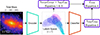 |
Fig. 1. Architecture and loss functions used in this paper. The input is the total mass and optionally X-ray maps that is then compressed using a convolutional NN (blue encoder) into a 7D latent space. From this latent space, we can get the similarity cluster and distance losses, Equations 1 and 3, or further transform it using a fully connected NN (red classifier) to obtain the classification loss, Equation 2. All losses are then weighted summed using the weights λCCLP, λdist, and λclass, Equation 4. See Figure B.1 for the full encoder and classifier architecture. |
The encoder does the bulk of the computation, and therefore, has the most complex architecture. The architecture follows the standard shape found in many convolutional NNs where the number of convolutional filters in a layer increase as the input is downscaled; however, the main difference is that we stack blocks of Inception modules (Szegedy et al. 2015) rather than individual convolutional layers and use max pooling for downscaling the input. After the Inception and max pool layers, there are two linear layers to form the cluster latent space. The classifier is much simpler and is composed of just two linear layers. To prioritise the most important features in the first dimensions, we add an information-ordered bottleneck layer (Ho et al. 2023) between the encoder and latent space. The information-ordered bottleneck zeros out all latent dimensions greater than k, where k is a random integer given by 1 ≤ k < |𝒵|, this results in the first dimensions representing the most important features as these will have the greatest chance of contributing to the loss function without being zeroed-out, with subsequent dimensions representing less important features. To introduce non-linearity into the network, we used the following activation functions: exponential linear units (ELUs) (Clevert et al. 2015) for convolutional layers, and scaled exponential linear units (SELUs) (Klambauer et al. 2017) for linear layers. For convolutional layers, we used a dropout probability of 5% to reduce overfitting (Srivastava et al. 2014).
To save on computational resources, some of our tests used a smaller encoder architecture that only uses standard convolutional layers instead of Inception modules, enabling us to perform more tests and increase ensemble learning to reduce NN stochastic uncertainties. We used the same activation functions as for the full architecture, but we changed the dropout probability to 10% for both convolutional and linear layers. This reduced NN will be used in the tests performed during the method section of this paper, while the full NN will be used for the results section, unless otherwise stated. The total number of parameters for the full architecture is 3 443 156, while the number of parameters in the reduced architecture is 232 204.
We chose |𝒵| = 7 to balance interpretability (which favours lower dimensionality) and network accuracy (which benefits from higher dimensionality). To determine the optimal number of dimensions, we trained five reduced NNs per combination of latent dimensions, X-ray inclusion, and number of simulations. We trained NNs with datasets starting with just BAHAMAS-0 and BAHAMAS-SIDM (solid), then adding BAHAMAS-AGN (dashed), and finally adding DARKSKIES (dotted). Figure 2 shows the average classification accuracy, normalised to the asymptotic accuracy, against the number of latent dimensions for the two datasets. To determine the point of diminishing returns, we fitted an arctan function, y = a + arctan((|𝒵|−b)/c), to each training set. We found that the number of the latent dimensions, |𝒵|, required to achieve 98% of the asymptotic accuracy for BAHAMAS without X-rays is 0.9, if we add X-rays, this then increases to 1.4. If we add BAHAMAS AGN, we find |𝒵| increases to 1.6 and 2.3 for X-rays excluded and included, respectively. Finally, adding DARKSKIES further increases |𝒵| to 6.3 and 3.3 for X-rays excluded and included, respectively. These results demonstrate that the required dimensionality grows with the degrees of freedom. The main outlier lies with the addition of DARKSKIES where excluding X-rays requires a larger |𝒵|. This is likely due to the difference in X-ray maps between BAHAMAS and DARKSKIES reducing the maximum classification accuracy from 59% to 48% with the exclusion of X-rays; therefore, flattening the best fit and increasing |𝒵| required to achieve 98% of asymptotic accuracy. Since |𝒵| ∼ 7 achieves at least 98% of the asymptotic accuracy for all scenarios, we adopt this value for the remainder of the paper.
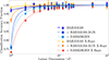 |
Fig. 2. Average classification accuracy from five NNs, normalised to the asymptotic accuracy, against the number of latent dimensions. Two sets of NNs are trained, one with X-rays included (reds/triangles) and the other excluded (blues/non-triangles). Each line shows an increase in the number of simulations included in the training, starting with BAHAMAS-0 and BAHAMAS-SIDM (solid), then BAHAMAS-AGN (dashed), and finally DARKSKIES (dotted). We fitted each set of data with an y = a + arctan((|𝒵|−b)/c) fit (lines). |
Previous work by H24 used Inception-v4; however, the motivation for moving away from Inception-v4 in this work to a custom architecture is that its performance in regression-based tasks for our data was sub-optimal, likely due to the large downscaling effect of the stem module that takes the input images of dimension (100×100) down to (10×10); therefore, almost all spatial information is lost at the beginning of the NN, leading to our more controlled downscaling, allowing more spatial information to be captured. However, more advanced architectures could be explored for potentially improved performance such as ConvNeXt (Liu et al. 2022) and vision transformers (Liu et al. 2021).
3.3. Training
We split the data into training and validation sets in a 4:1 ratio to prevent overfitting. The NN is trained on the training set by minimising the loss and updating its parameters via backpropagation, while the validation set is used to evaluate generalisation performance of the NN on unseen data and tune hyperparameters. We treat the validation fraction of the unknown dataset as the test dataset that we want to obtain σDM/m for, as our method can leverage information from the unknown dataset to help inform its estimations. We exclude the DARKSKIES simulations from hyperparameter tuning to prevent any biases in our results.
We used the PyTorch (Ansel et al. 2024) library for implementing NNs, with the AdamW optimiser (Loshchilov & Hutter 2017) for stochastic gradient descent with a learning rate of 10−4. We implemented a learning rate scheduler that reduces the learning rate by half if the validation loss does not improve by at least 10% over ten epochs, which encourages fast initial convergence, while enabling more precise optimisation near minima. In order to improve convergence time, we normalise the data to be of order of one, with the input image maps each normalised to a maximum value of one and for σDM/m, we take the logarithmic transform and normalise so that log(σDM/m) lies between zero and one. We train with a batch size of 120 on an NVIDIA RTX 4080 GPU with 16 GB of video memory. Due to the reduced number of parameters in the reduced NN, the computational time is reduced by a factor of three, enabling us to carry out more calibration tests.
3.4. Estimating σDM/m and confidence
For each galaxy cluster in the validation set we got an estimate for σDM/m, with all galaxy cluster estimations in one simulation forming a distribution for σDM/m, representing uncertainty due to data variation. We then calculated the PDF using a Gaussian kernel. However, NNs introduce additional uncertainty due to their stochastic nature, including randomly weight initialisation, dropout, and mini-batches. To capture the NN uncertainty, we employed ensemble learning (Dasarathy & Sheela 1979; Dong et al. 2020), training multiple NNs with different initialisations. We then combined the NNs estimated PDFs for σDM/m by taking the product to account for NN uncertainty.
In order to quantify our confidence in an estimation, we can use the more expressive latent space to identify whether a test dataset falls outside the training domain, resulting in untrustworthy estimations. Qualitatively, if a test dataset forms a cluster far from those of the training datasets in the latent space, we can conclude that there are few if any shared features, suggesting extrapolation was performed and the dataset lies outside the training domain. While the information-ordered bottleneck orders the latent space in terms of importance, there are still degenerate dimensions; therefore, we can also apply principal component analysis (PCA) (Pearson 1901; Hotelling 1933) to more effectively visualise the dominant features. PCA works by finding a new set of orthogonal bases, where the first basis explains the most variance in the data, followed by subsequent dimensions.
To quantify the confidence that the test set lies within the training domain, we projected all non-physical latent dimensions (i.e. all but the first), along the axis connecting the centroid of the test set to each known dataset. We excluded the first dimension to avoid biasing the estimate of σDM/m towards any particular simulation. We assessed the confidence by measuring the degree of overlap between the known and test projected distributions. We also experimented with different confidence metrics, including the Earth mover distance (Rubner et al. 1997, 2000), KS-test, and NN classification accuracy; however, the overlap proved the most interpretable and gave the largest dynamic range.
4. Results
In this section we present the results from variety of tests. The aim of this section is to present how compact clustering can lead to robust and confident estimates of the cross-section, moreover it can aid interpretability.
4.1. Self-organising latent space for robust inference
To demonstrate the interpretability of our model, we first trained and tested on BAHAMAS only. In this case (and only this case), we used two input channels, the total mass maps, but also an additional X-ray channel. The X-ray maps are taken from H24, which used methods from Le Brun et al. (2014) to generate realistic X-ray emission maps. We trained on all fiducial BAHAMAS models (BAHAMAS-0 and BAHAMAS-SIDM), and we treated both the strong and weak AGN variants (BAHAMAS-0s and BAHAMAS-0w, respectively) as unknown.
Figure 3 shows the first two components from PCA. The training data are shown with solid contours and projected histograms, while the unlabelled test data use hatched contours and histograms. We also denote the test data with an asterisks in the legend. Due to ℒdist, the optimisation process organises the latent space such that training samples with different σDM/m extend along the first principal component. The estimated σDM/m for BAHAMAS-0w and BAHAMAS-0s is  ,
,  , respectively, with BAHAMAS-0 having
  , resulting in over an order of magnitude difference in estimated σDM/m for the three CDM simulations. The unlabelled test data with zero cross-section aligns with the BAHAMAS-0 cluster in the first component; however, subtle differences cause the strong and weak AGN variants to deviate from BAHAMAS-0, extending primarily along the second principal component, orthogonal to σDM/m. Looking at the second component, we see BAHAMAS-SIDM and BAHAMAS-0 line along the same line with BAHAMAS-0 and BAHAMAS-1 having values of
  and −0.29 ± 0.45, respectively, while BAHAMAS-0w and BAHAMAS-0s have offsets of
  and
and  , respectively. The first two components have an explained variance ratio of 47% and 28%, respectively, for a total explained variance ratio of 75%.
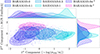 |
Fig. 3. First two components of the PCA of the 7D latent space. Each point corresponds to a galaxy cluster from its colour corresponding simulation with the contours representing the 68% region for that simulation. The unknown datasets, BAHAMAS-0w and BAHAMAS-0s, are represented by the hatched contours and asterisk next to the legend label. We interpret that the first component corresponds to a transformation of log(σDM/m) and the second component corresponds to the level of AGN feedback. |
This reveals two key insights. First, the second principal component captures the level of AGN feedback in the simulations without any prior labelling. Second, the extracted features appear to be orthogonal to those associated with σDM/m, similar to what H24 found. Since our primary focus is on estimating confidence in σDM/m, we omit the X-ray channel moving forward, as it only contributes to interpretability and not constraining power in σDM/m. Future work may explore the use of X-rays to study AGN feedback in clusters; however, this is beyond the scope of this work.
4.2. Testing on out-of-domain data: Random noise
Having demonstrated the flexibility of our self-organising latent space, we now test its ability to recognise out-of-domain (OOD) features. In traditional regression models (cf. H24), estimations are often accurate and precise on training and in-domain test data; however, if the test set is OOD, these models lack any mechanism to indicate this mismatch, resulting in estimations that cannot be trusted. As a result, they often return overly confident estimations.
To test this hypothesis, we constructed a simple test case using completely random noise, where each pixel is sampled from a uniform distribution between 0 and 1, and hence contains no signal. We expect that this will manifest as anomalous structure in the latent space, whereas traditional regression would return an estimate regardless. We trained both the clustering-based and traditional regression models using a reduced architecture, training each model ten times for 150 epochs. The architectures are identical up to the final layer and the information-ordered bottleneck. In the clustering-based model, the final layer outputs a probability for each class, with σDM/m derived from the latent space. In the regression model, the final layer directly outputs a single σDM/m value. The NNs are trained on the fiducial BAHAMAS simulations only. For the clustering regression the noise is treated as unknown during training, while it is not used during training in the traditional regression NN.
The left panel of Figure 4 shows the combined estimated distributions from the ten runs from traditional regression, with the BAHAMAS simulations shown in shades of blue and noise shown in hatched black. The NN estimates  ,
,  , 0.350 ± 0.070 cm2 g−1, and
  for BAHAMAS-0, BAHAMAS-0.1, BAHAMAS-0.3, and BAHAMAS-1, respectively. For the noise dataset, it is incorrectly assigned a physically meaningful value of
  .
.
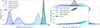 |
Fig. 4. Method of building confidence in our ML estimator for data outside the training domain. Left: Train ensemble of ten regression NNs on the fiducial hydro BAHAMAS simulations. We show the combined PDF of log(σDM/m) for the known BAHAMAS simulations (blue shades) and blind uniform random noise (hatched black). We find that the regressor consistently estimates a significant, positive cross-section of ∼0.6 cm2g−1 with no regard to its confidence, presenting the issue with direct regression estimators. Right: First and third latent dimensions from our compact clustering algorithm trained with the same fiducial BAHAMAS as known (blue shades) and the random noise dataset as unknown (hatched black). The first latent dimension corresponds to log σDM/m, which we would naively assume that the noise dataset has a cross-section of ∼0.1 cm2 g−1; however, from the third dimension we see that the noise dataset shares no similarities with the known simulations and therefore, cannot be trusted. |
In contrast, the clustering model allows us to examine the latent space directly. The right panel of Figure 4 shows the σDM/m dimension and the third latent dimension for different datasets, for one representative run. We choose the third latent dimension as this shows the greatest separation between the noise and the BAHAMAS simulations. From the top left subplot that corresponds to σDM/m, we find σDM = 0.118 ± 0.007 cm2 g−1 for the noisy dataset taken from ten runs. The third dimension, far right subplot, shows clear separation between the noise and BAHAMAS simulations with no shared features, confirming that the noise lies outside the training domain. We quantitively measure this by projecting the distribution of values in the direction from the centre of each BAHAMAS cluster to the centre of the noisy data. This projection allows us to estimate the overlap between the noise and each simulation cluster. We find that the overlap is consistent with zero, confirming that the noise dataset is recognised as OOD.
4.3. Confidence on in-domain data
Having shown that our compact clustering method can self-organise its latent space to produce a confidence estimate in our estimations, we move to a more realistic scenario. To evaluate the model’s ability to report confidence in realistic OOD test data, we first assessed its performance on an in-domain test set. Specifically we trained on the fiducial BAHAMAS simulations with BAHAMAS-0.1 treated as unknown. We train the full architecture three times for 150 epochs each to construct an ensemble. The left hand panel of Figure 5 shows the results of the validation set on the known simulations (solid colours) and the unknown test set, BAHAMAS-0.1 (hatched black). The legend marks the test label with an asterisk. The NN estimates σDM/m of  ,
,  , and
, and  for BAHAMAS-0, BAHAMAS-0.3, and BAHAMAS-1, respectively, while for the unknown BAHAMAS-0.1, the NN estimates
  . However, the BAHAMAS-0.1 is bimodal, which leads to the wide confidence range. Due to our feature-based clustering, several physical features correlate with the effective strength of self-interaction, such as the mass of the galaxy cluster or the dynamical state. This results in some SIDM0.1 halos (low mass halos for example) appearing indistinguishable from CDM. Since the loss function acts to separate clusters based on feature similarity, it can create two populations resulting in a bimodal distribution for SIDM0.1. This is more pronounced when the unphysical choice for CDM is very far from 0.1, dragging those low-mass halos in SIDM0.1 away from its true value and creating a bimodal distribution. The right hand panel of Figure 5 shows the 1D projected latent space. We see that the in-domain unknown test set has a significant overlap of 48.8 ± 0.3 % and 55.3 ± 1.0 % with the BAHAMAS-0 and the BAHAMAS-0.3 simulations, respectively, reflecting the model’s confidence in its estimation and its similarity to these datasets.
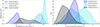 |
Fig. 5. Consistency check on in-distribution testing. Left: Trained ensemble of three clustering NNs and combined PDF of log(σDM/m) for the known BAHAMAS-0, BAHAMAS-0.3, and BAHAMAS-1 (solid blue shades) and unknown BAHAMAS-0.1 (dashed black). We find a cross-section of ∼0.05 cm2 g−1 and within 1σ of 0.1 cm2 g−1 for BAHAMAS-0.1. Right: Projected 7D latent space from our clustering algorithm into a 1D distance PDF, where each known simulation (blue shades) is projected in the direction from the centre of their distribution to the centre of BAHAMAS-0.1. BAHAMAS-0.1 (hatched black) is projected in the direction of BAHAMAS-0.3 to show the greatest overlap. The distance has arbitrary units as it depends on the scale of the latent space. BAHAMAS-0.1 shares a large overlap of 49% and 55% with BAHAMAS-0 and BAHAMAS-0.3, respectively, leading to the conclusion that it lies within the training domain. |
We repeated the process with BAHAMAS-0.3 treated as the unknown dataset and BAHAMAS-0.1 included in the training set. The NN estimates σDM/m of  ,
,  , and
, and  for BAHAMAS-0, BAHAMAS-0.1, and BAHAMAS-1, respectively, while for the unknown BAHAMAS-0.3, the NN estimates
  . We see that the unknown BAHAMAS-0.3 also has a significant overlap of 59.9 ± 0.3 % with the BAHAMAS-0.1 simulation, higher than for BAHAMAS-0.1 as the unknown, possibly explaining the lower log uncertainties and non-bimodal posterior.
Next, we introduce additional CDM simulations, BAHAMAS-0w and BAHAMAS-0s, that differ in their level of AGN feedback. All the previous BAHAMAS simulations are now known, while the extra BAHAMAS-CDM simulations are given unique unknown labels. Figure 6 shows the distributions of each simulation in the direction towards BAHAMAS-0w. We show the projection of the BAHAMAS-0w distribution along the direction towards BAHAMAS-0 that exhibits the greatest overlap with a known class. An analogous figure can be produced for BAHAMAS-0s that produces qualitatively similar results. The estimated σDM/m for BAHAMAS-0w and BAHAMAS-0s are  and
and  , respectively. For BAHAMAS-0w, the maximum overlap is 83.9 ± 0.6 % with BAHAMAS-0, while for BAHAMAS-0s, the maximum overlap is 90.1 ± 1.3 % with BAHAMAS-0. The overlap between the two AGN simulations is 77.1 ± 0.7 %.
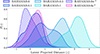 |
Fig. 6. 7D latent space projection from our clustering algorithm into a 1D distance PDF, where each known simulation and BAHAMAS-0s is projected in the direction from the centre of their distribution to the centre of BAHAMAS-0w (blue shades and pink hatched). BAHAMAS-0w is projected in the direction of BAHAMAS-0 to show the greatest overlap (purple hatched). The distance has arbitrary units as it depends on the scale of the latent space. BAHAMAS-0w shares a large overlap with BAHAMAS-0, leading to the conclusion that it lies within the training domain. |
4.4. Realistic out-of-domain data
Finally, we want to observe the effect of choosing a realistic dataset that is initially outside the training domain, and how adding additional simulations progressively brings the test set into the training domain. To do this we set the unknown dataset as DARKSKIES-0.1 throughout. We initially train three models over 150 epochs on the fiducial BAHAMAS set, with DARKSKIES-0.1 as the unknown dataset. We estimate the cross-section (where the truth is σDM = 0.1 cm2 g−1), project the latent space, and calculate the overlap integral with the most similar simulation. We then rerun the training, with each time including more simulations: BAHAMAS + AGN, then DARKSKIES-0, and finally DARKSKIES-0.2. In the case of DARKSKIES-0 we are forced to give it a value for σDM/m; therefore, we motivate our selection for CDM simulations to be in line with the effective σDM/m found in Harvey et al. (2019). Although DARKSKIES is significantly higher resolution than BAHAMAS, we do not want the model to distinguish differences within CDM simulations. In fact, we want it to learn to align all CDM simulations, so we assigned DARKSKIES-0 the same classification label as BAHAMAS-0. Since this σDM/m represents the upper limit of the model’s ability to distinguish SIDM from CDM, this assignment should not introduce any bias.
The left-hand panel of Figure 7 shows the combined probability distributions of σDM/m for each simulation in the final trained NN including all datasets. Blue shades correspond to BAHAMAS simulations and red shades to DARKSKIES, with the unknown test DARKSKIES-0.1 represented by black hatching. The BAHAMAS simulations are estimated to have σDM/m of  ,
,  ,
,  , and
, and  for BAHAMAS-0, BAHAMAS-0.1, BAHAMAS-0.3, and BAHAMAS-1, respectively. For the DARKSKIES simulations, the estimations are
  and
and  for DARKSKIES-0 and DARKSKIES-0.2, respectively, and for the unknown test DARKSKIES-0.1, the NN estimates
  .
.
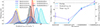 |
Fig. 7. Adaptation to a new domain. Left: Train ensemble of five clustering NNs with BAHAMAS, DARKSKIES-0, and DARKSKIES-0.2 as known (solid blue and red shades) and DARKSKIES-0.1 as unknown (hatched black). We show the combined PDF of log(σDM/m) from the five runs. We find a cross-section of ∼0.14 cm2 g−1 for DARKSKIES-0.1, within 1σ of 0.1 cm2 g−1. Right: Overlap confidence (left axis, solid blue), estimated σDM/m (right axis, dashed purple), and target σDM/m (right axis, dotted black) for DARKSKIES-0.1 as we progressively add known simulations during training. We start with BAHAMAS-0 and BAHAMAS-SIDM, then add the BAHAMAS-AGN simulations, DARKSKIES-0, and finally DARKSKIES-0.2. We see that the overlap confidence closely follows the convergence of DARKSKIES-0.1 onto the target σDM/m with an overlap of 70% resulting in DARKSKIES-0.1 being within 1σ of the target σDM/m. |
The right-hand panel of Figure 7 shows the largest overlap between DARKSKIES-0.1 and the known simulations, on the right-hand y axis, along with the estimated σDM/m on the left-hand y axis, for each set of training simulations. As the overlap increases, the estimation converges towards the correct cross-section, with an overlap of 70.5 ± 1.3 % resulting in an estimate within 1σ of the target value. DARKSKIES-0.1 has zero overlap with the BAHAMAS simulations, which could be the reason for the large error when DARKSKIES-0.2 is not included as BAHAMAS is not able to provide sufficient upper limit support.
5. Discussion
We have presented a semi-supervised clustering algorithm that provides both confidence estimation and interpretability for constraints on the DM self-interaction cross-section. We demonstrate that the model can identify additional physical features in the dataset, detect out-of-domain data, and constrain idealised observations in a σDM/m = 0.1 cm2 g−1 universe. However, several aspects remain that require further discussion and development.
5.1. Interpreting the self-organising latent space
We first show in Figure 3 that clustering in a high-dimensional latent space allows us to analyse the model’s learned features, using either an information-ordered bottleneck layer or PCA. We can directly observe how the model is learning different levels of baryonic feedback compared to σDM/m. However, without methods to identify how the NN is learning or without a well sampled latent space, interpreting what physical properties each latent dimension represents can be challenging and uncertain. This is often due to the fact that physical features do not extend linearly along individual latent dimensions; rather, each latent feature may correspond to a non-linear combination of the simulation properties. In the case of Figure 3, where AGN feedback and σDM/m were the only varying parameters, the latent features were relatively straightforward to interpret.
To improve interpretability, additional simulations spanning a wider range of parameter space are needed to cross-correlate physical properties with latent features. It may also be beneficial to use methods that can directly identify which input features the NN uses to inform its estimations, such as feature importance, activation maps, counterfactual examples, or generative models.
Another avenue for improvement is how the network learns to cluster data. Currently, latent vector similarity is minimised or boosted if they share the same class; however, using a class-level similarity metric, including physical properties, such as a self-interaction cross-section; summary statistics, such as density profiles; or features extracted from NNs, this could provide a more robust method for clustering based on feature similarity.
5.2. Confidence estimation
We show that high-dimensional latent spaces provide a natural means to measuring similarity and detect out-of-domain datasets. We can use different metrics of measuring similarity, such as overlap, earth mover distance (EMD), KS-test, and classification accuracy. Each metric has its own advantages and limitations. Overlap, EMD, and the KS-test require, in the simplest form, 1D projects, while classification accuracy operates in the full latent space and arises naturally from our architecture, albeit as an approximation. Classification accuracy and overlap are the most interpretable, while EMD is the most sensitive at the extremes of very high or very low similarity. Ultimately, we adopt overlap as our primary metric due to its simplicity, interpretability, and effectiveness as a proxy for similarity. However, future work will explore more robust metrics, including higher-dimensional overlap and methods that account for similarity across multiple reference datasets.
5.3. Application to real data and reducing uncertainties
Our ultimate goal is to constrain σDM/m in our Universe; therefore, before we can pass observations to our NN, we must first forward model our total mass maps into realistic weak lensing convergence or shear maps, incorporating instrumental effects, Fourier boundary artifacts from the shear-to-convergence transformation, and statistical noise. This degradation will inevitably increase the uncertainty in our estimated σDM/m values and reduce our constraining power. Future work will aim to reduce these uncertainties by:
-
Adding more simulations to improve generalisation, especially in new domains.
-
Using higher-resolution simulations with greater parameter space coverage.
-
Training for more epochs and train more NNs for improved ensemble learning.
-
Improving the NN architecture with features from models such as vision transformers or ConvNeXt.
Another important consideration is how we handle the non-physical value of σDM/m assigned to CDM. While SIDM simulations follow σDM/m ≫ 0.01 cm2 g−1, the arbitrary CDM σDM/m does not currently cause significant bias; however, future simulations approaching this threshold may require us to exclude low-resolution CDM simulations if they introduce confusion with SIDM models.
5.4. Comparison with simulation based inference methods
Simulation-based inference (SBI) is a powerful approach for learning posteriors or likelihoods directly from simulations, providing uncertainty estimates for individual observations. However, SBI typically operates on per-sample posteriors, whereas in cosmology, macroscopic parameters, such as the dark matter self-interaction cross-section, are generally constrained through observational ensembles. While our method shares many similarities with traditional SBI through the use of simulations to obtain posteriors for parameters, it differs by aggregating predictions from many observations to recover a posterior for a macroscopic parameter, even in sparsely sampled domains where traditional ML methods, including SBI, struggle to interpolate.
5.5. Domain variance and adaptation
It is clear from Figure 7 that the clustering algorithm in its current state does not generalise well beyond that of its training domain, unable to predict the cross-section in the DARKSKIES suite of simulations, a common problem in ML. In the scope of this work we required an algorithm that did not generalise well in order to evidence how it worked (should it have been perfectly generalised, the right-hand side of Figure 7 would be flat). However, even in the case where there was perfect generalisation we would still require empirical insight when applied to real observations to inform us of the model’s confidence in its estimates. Therefore, our method and domain adaptation are complementary and both will need to be combined before we apply this to data to identify if the domain adaption is correctly aligning the features in the two domains, which we will show in future work.
6. Conclusions
We have presented a ML method of measuring the dark matter self-interaction cross-section, σDM/m, from 2D gravitational lensing mass maps that can return robust confidence limits in its estimates. Since we cannot observe multiple universes with different σDM/m, we must rely on simulations for inference. However, simulations do not perfectly replicate observations, which presents a challenge for simulation-based inference. We have developed a clustering NN architecture capable of recovering macroscopic parameters in a sparsely sampled parameter space while producing an interpretable latent space that provides a metric for assessing the confidence of estimations on unknown datasets. The NN learns features from both known and unknown datasets during training, enabling it to cluster samples based on their similarities in a high-dimensional latent space.
Through a series of targeted tests, we show that when observations resemble the training domain, our method can recover σDM/m within 1σ, even with limited simulated coverage of the parameter space. The high-dimensional latent space also enables exploration of secondary physical features, such as variations in black-hole feedback, even when these are not explicitly labelled during training. Furthermore, by expressing the latent space in higher dimensions and measuring the projected overlap between different domains, we can quantify estimation confidence. This estimation confidence allows us to determine whether a dataset lies within the training domain, suggesting shared features and reliable interpolation, or is out-of-domain, indicating the dataset is foreign with potential extrapolation and unreliable estimations. We demonstrate that when presented with a dataset of uniform noise, the network correctly identifies it as out-of-domain relative to the BAHAMAS simulations. Finally, we show that if our observations, DARKSKIES-0.1, belong to a different suite of simulations without prior exposure, the NN fails to recover the target σDM/m. However, by leveraging higher dimensions and similarity metrics, we show that NNs can still be used in trustworthy ways for scientific inference.
Our next steps will be to move towards applying this architecture to real observations to obtain a constraint competitive with traditional methods for σDM/m. As such, it will be essential to generate realistic mock observations from simulations, incorporating instrumental noise and observational effects. We also aim to train on a broader range of cosmological simulations to better sample the latent space and marginalise over non-physical differences across simulation suites. For future improvements, we aim to incorporate domain adaptation techniques to reduce the performance gap on datasets that differ from the training domain. Finally, we can explore methods for NN interpretability to gain deeper insight into what the NN is learning, further improving trust of ML in science.
The method we have presented here represents a blueprint for the use of ML in scientific inference. The flexibility of compact clustering to manipulate the learned features amongst a variety of different simulation suites enables us to build an enriched latent-space that incorporates a host of different simulations. This way we can numerically marginalise over all unknowns, delivering robust and trustworthy inference of cosmological parameters.
Data availability
Data from McCarthy et al. (2017), Robertson et al. (2019), Harvey et al. (2025) for the BAHAMAS and DARKSKIES simulations are available on request from the original authors. Access to the code and trained weights of the neural networks can be found via https://github.com/EthanTreg/Bayesian-DARKSKIES.
Acknowledgments
This work was supported by the Swiss State Secretariat for Education, Research and Innovation (SERI) under contract number 521107294. We would like to thank Andrew Robertson and Ian McCarthy for developing the BAHAMAS-SIDM simulations.
References
- Ansel, J., Yang, E., He, H., et al. 2024, in 29th ACM International Conference on Architectural Support for Programming Languages and Operating Systems (ASPLOS ’24) (ACM), 2 [Google Scholar]
- Bode, P., Ostriker, J. P., & Turok, N. 2001, ApJ, 556, 93 [Google Scholar]
- Burles, S., & Tytler, D. 1998, ApJ, 499, 699 [Google Scholar]
- Carlson, E. D., Machacek, M. E., & Hall, L. J. 1992, ApJ, 398, 43 [CrossRef] [Google Scholar]
- Caron, M., Bojanowski, P., Joulin, A., & Douze, M. 2018, in Proc. European Conference on computer vision (ECCV), 132 [Google Scholar]
- Clevert, D. A., Unterthiner, T., & Hochreiter, S. 2015, ArXiv preprint [arXiv:1511.07289] [Google Scholar]
- Clowe, D., Bradač, M., Gonzalez, A. H., et al. 2006, ApJ, 648, L109 [NASA ADS] [CrossRef] [Google Scholar]
- Copi, C. J., Schramm, D. N., & Turner, M. S. 1995, Science, 267, 192 [CrossRef] [PubMed] [Google Scholar]
- Correa, C. A., Schaller, M., Ploeckinger, S., et al. 2022, MNRAS, 517, 3045 [NASA ADS] [CrossRef] [Google Scholar]
- Dasarathy, B., & Sheela, B. 1979, Proc. IEEE, 67, 708 [Google Scholar]
- Davis, M., Huchra, J., Latham, D. W., & Tonry, J. 1982, ApJ, 253, 423 [NASA ADS] [CrossRef] [Google Scholar]
- de Laix, A. A., Scherrer, R. J., & Schaefer, R. K. 1995, ApJ, 452, 495 [Google Scholar]
- Dong, X., Yu, Z., Cao, W., Shi, Y., & Ma, Q. 2020, Front. Comput. Sci., 14, 241 [Google Scholar]
- Euclid Collaboration (Aussel, B., et al.) 2024, A&A, 689, A274 [NASA ADS] [CrossRef] [EDP Sciences] [Google Scholar]
- Hartigan, J. A., & Wong, M. A. 1979, J. Royal Stat. Soc. Ser. c (Appl. Stat.), 28, 100 [Google Scholar]
- Harvey, D. 2024, Nat. Astron., 8, 1332 [Google Scholar]
- Harvey, D., Robertson, A., Massey, R., & McCarthy, I. G. 2019, MNRAS, 488, 1572 [NASA ADS] [CrossRef] [Google Scholar]
- Harvey, D., Revaz, Y., Schaller, M., et al. 2025, A&A, Submitted [Google Scholar]
- Hinshaw, G., Larson, D., Komatsu, E., et al. 2013, ApJS, 208, 19 [Google Scholar]
- Ho, M., Zhao, X., & Wandelt, B. 2023, ArXiv preprint [arXiv:2305.11213] [Google Scholar]
- Hotelling, H. 1933, J. Educational Psychol., 24, 417 [CrossRef] [Google Scholar]
- Hoyle, B. 2016, Astron. Comput., 16, 34 [NASA ADS] [CrossRef] [Google Scholar]
- Huertas-Company, M., & Lanusse, F. 2023, PASA, 40 [Google Scholar]
- Ivezić, Ž., Kahn, S. M., Tyson, J. A., et al. 2019, ApJ, 873, 111 [Google Scholar]
- Johnson, T. L., Sharon, K., Bayliss, M. B., et al. 2014, ApJ, 797, 48 [Google Scholar]
- Kamnitsas, K., Castro, D., Folgoc, L. L., et al. 2018, Proc. Mach. Learn. Res., 80, 2459 [Google Scholar]
- Kim, S. Y., Peter, A. H. G., & Wittman, D. 2017, MNRAS, 469, 1414 [NASA ADS] [CrossRef] [Google Scholar]
- Klambauer, G., Unterthiner, T., Mayr, A., & Hochreiter, S. 2017, in Advances in Neural Information Processing Systems, 30 [Google Scholar]
- Laureijs, R., Gondoin, P., Duvet, L., et al. 2012, SPIE Conf. Ser., 8442, 84420T [Google Scholar]
- Le Brun, A. M. C., McCarthy, I. G., Schaye, J., & Ponman, T. J. 2014, MNRAS, 441, 1270 [NASA ADS] [CrossRef] [Google Scholar]
- Liu, Z., Lin, Y., Cao, Y., et al. 2021, Proceedings of the IEEE/CVF International Conference on Computer Vision, 10012 [Google Scholar]
- Liu, Z., Mao, H., Wu, C.-Y., et al. 2022, Proceedings of the IEEE/CVF Conference on Computer Vision and Pattern Recognition, 11976 [Google Scholar]
- Loshchilov, I., & Hutter, F. 2017, ArXiv preprint [arXiv:1711.05101] [Google Scholar]
- McCarthy, I. G., Schaye, J., Bird, S., & Le Brun, A. M. C. 2017, MNRAS, 465, 2936 [Google Scholar]
- Merten, J., Giocoli, C., Baldi, M., et al. 2019, MNRAS, 487, 104 [Google Scholar]
- Oman, K. A., Navarro, J. F., Fattahi, A., et al. 2015, MNRAS, 452, 3650 [CrossRef] [Google Scholar]
- Peacock, J. A., Cole, S., Norberg, P., et al. 2001, Nature, 410, 169 [Google Scholar]
- Pearson, K. 1901, London, Edinburgh. Dublin Philos. Magaz. J. Sci., 2, 559 [Google Scholar]
- Peter, A. H. G., Rocha, M., Bullock, J. S., & Kaplinghat, M. 2013, MNRAS, 430, 105 [Google Scholar]
- Planck Collaboration VI. 2020, A&A, 641, A6 [NASA ADS] [CrossRef] [EDP Sciences] [Google Scholar]
- Ren, Y., Pu, J., Yang, Z., et al. 2022, ArXiv e-prints [arXiv:2210.04142] [Google Scholar]
- Richard, J., Jauzac, M., Limousin, M., et al. 2014, MNRAS, 444, 268 [Google Scholar]
- Robertson, A., Massey, R., & Eke, V. 2017, MNRAS, 465, 569 [NASA ADS] [CrossRef] [Google Scholar]
- Robertson, A., Harvey, D., Massey, R., et al. 2019, MNRAS, 488, 3646 [NASA ADS] [CrossRef] [Google Scholar]
- Roche, C., McDonald, M., Borrow, J., et al. 2024, Open J. Astrophys., 7, 65 [Google Scholar]
- Rubin, V. C., Ford, Jr., W. K., & Thonnard, N. 1978, ApJ, 225, L107 [NASA ADS] [CrossRef] [Google Scholar]
- Rubin, V. C., Ford, Jr., W. K., & Thonnard, N. 1980, ApJ , 238, 471 [NASA ADS] [CrossRef] [Google Scholar]
- Rubner, Y., Guibas, L. J., & Tomasi, C. 1997, Proc. ARPA image Understanding Workshop, 661, 668 [Google Scholar]
- Rubner, Y., Tomasi, C., & Guibas, L. J. 2000, Int. J. Comput. Vision, 40, 99 [CrossRef] [Google Scholar]
- Sagunski, L., Gad-Nasr, S., Colquhoun, B., Robertson, A., & Tulin, S. 2021, JCAP, 2021, 024 [CrossRef] [Google Scholar]
- Sen, S., Agarwal, S., Chakraborty, P., & Singh, K. P. 2022, Exp. Astron., 53, 1 [NASA ADS] [CrossRef] [Google Scholar]
- Sirks, E. L., Harvey, D., Massey, R., et al. 2024, MNRAS, 530, 3160 [Google Scholar]
- Spergel, D. N., & Steinhardt, P. J. 2000, Phys. Rev. Lett., 84, 3760 [NASA ADS] [CrossRef] [Google Scholar]
- Srivastava, N., Hinton, G., Krizhevsky, A., Sutskever, I., & Salakhutdinov, R. 2014, J. Mach. Learn. Res., 15, 1929 [Google Scholar]
- Szegedy, C., Liu, W., Jia, Y., et al. 2015, in Proceedings of the IEEE conference on computer vision and pattern recognition, 1 [Google Scholar]
- Szegedy, C., Ioffe, S., Vanhoucke, V., & Alemi, A. 2017, Proceedings of the AAAI conference on artificial intelligence [Google Scholar]
- Tzoreff, E., Kogan, O., & Choukroun, Y. 2018, ArXiv e-prints [arXiv:1805.10795] [Google Scholar]
- White, S. D. M., Davist, M., Efstathioui, G., & Frenk, C. S. 1987, Nature, 330, 451 [NASA ADS] [CrossRef] [Google Scholar]
- Yang, X., Deng, C., Zheng, F., Yan, J., & Liu, W. 2019, Proceedings of the IEEE/CVF Conference on Computer Vision and Pattern Recognition (CVPR) [Google Scholar]
- Zwicky, F. 2009, General Relativ. Gravit., 41, 207 [Google Scholar]
Appendix A: Compact clustering via label propagation
In Section 3.1 we outline the three loss functions used in our method, with Equation 1 introduced by Kamnitsas et al. (2018). In this section, we derive the matrices T ∈ ℝN × N and H(s) ∈ ℝN × N, latent vectors Z ∈ ℝN × |𝒵|, and a set of class probabilities, Y′∈ℝN × C, for the set of classes, C, with batch size N and latent space 𝒵. A portion of the dataset is unlabelled, N = NL + NU, with latent vectors ZL and ZU, where L and U subscripts correspond to the labelled and unlabelled samples, respectively. As we want to find the transition and target transition matrices, H and T, we first generate a fully connected graph in the latent space by calculating the adjacency matrix, A ∈ ℝN × N from Equation A.1, where each element, Aij, is the weight of an edge in the graph and represents the similarity between samples i and j.
 (A.1)
(A.1)
We then row-wise normalise A, Equation A.2, so that each element of the transition matrix, Hij, is the probability of a transition from sample i to sample j.
 (A.2)
(A.2)
We structure H so that the labelled and unlabelled samples are arranged as Equation A.3.
![Mathematical equation: $$ \mathbf H = \left[{\begin{matrix} {\mathbf H} _{LL} & {\mathbf H} _{UL} \\ {\mathbf H} _{LU} & {\mathbf H} _{UU} \end{matrix}}\right] $$](/articles/aa/full_html/2026/01/aa56629-25/aa56629-25-eq36.gif) (A.3)
(A.3)
From H, we can propagate labels from the known samples to the unknown samples based on their probability of transition, forming the class posterior matrix ![Mathematical equation: $ \mathbf{\Phi}=\left[{\begin{matrix} &\mathbf{Y}_L \\ &{\mathbf{\Phi}}_U \end{matrix}}\right]\in\mathbb{R}^{N\times C} $](/articles/aa/full_html/2026/01/aa56629-25/aa56629-25-eq37.gif) , where YL ∈ ℝNL × C are the one hot vectors of the known class labels and
, where YL ∈ ℝNL × C are the one hot vectors of the known class labels and  is the unlabelled class posteriors given by Equation A.4.
 (A.4)
(A.4)
Then, from Φ, we can calculate T that acts as a soft target probability for a transition between two class labels, maximising same class transitions, while minimising inter-class transitions, given by Equation A.5.
 (A.5)
(A.5)
Finally, we want to minimise the cross-entropy between T and H; however, we can form Markov chains to enable class propagation along high density regions, preserving the structure of the graph. Therefore, the probability that a Markov process starts from sample i, performs (s−1) steps within the same class, and then transitions to sample j is given by Equation A.6.
 (A.6)
(A.6)
Where ° is the Hadamard product and M = ΦΦT ∈ ℝN × N is the probability that two samples belong to the same class, with HijMij being the approximate joint probability of transitioning from sample i to sample j and the two samples belonging to the same class. Therefore, we can construct ℒCCLP as the cross-entropy between the target transition, T, and the transition probability along the Markov chain, H(s) as shown in Equation 1. For more details see Kamnitsas et al. (2018).
Appendix B: Network architecture
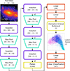 |
Fig. B.1. Full network architecture used in the paper. The network is composed of inception blocks (purple, rounded rectangles), show in Figure B.2, max pooling layers (turquoise, trapeziums), linear layers (red, rectangles), a flatten layer (yellow, rectangle), and an information-ordered bottleneck layer (yellow, rounded rectangle). The output dimensions of each layer is represented underneath the name of the layer, the arrows represent the direction of data flow and if there is a ×2 next to the arrow, then the layer is repeated twice. The input is the total mass maps and optionally X-ray maps of galaxy clusters and the latent space is where we calculate the loss functions from equations 1 and 3 as well as our feature analysis. |
We show in Figure B.1 the full architecture used in this paper. As mentioned in Section 3.2, the input is the total mass maps and optionally X-ray maps and the output is a 7D latent space and classification scores. The network is composed of inception blocks (purple, rounded rectangle), Figure B.2, max pooling (turquoise, trapeziums), and linear layers (red, rectangles). Some inception blocks are followed by a ×2 representing that this layer is repeated twice and the output shape from each layer is shown under the layer name with the last layer depending on the number of classes, |C|, used during training, which includes the number of both known and unknown simulations with unique σDM/m. The inception blocks use convolutional layers with different kernel sizes to learn spatial features within different receptive fields. The max pooling downscales the input with inception blocks following as this enables the convolutional layers within the inception blocks to learn features on different scales as each downscale increases the receptive field of the convolutional kernel. The flatten followed by linear layers converts the spatial domain to a regression and classification domain with a linear layer outputting seven features followed by an information-ordered bottleneck creating the latent space and two more linear layers after the latent space for the classification loss function. The information-ordered bottleneck aims to order the latent dimensions based on loss function importance, so the first dimensions should contribute the most to minimising the loss, and therefore, containing the most information, Figure D.1 shows an example of a 7D latent space. There are many more advanced network architectures used in computer vision; however, we found worse performance when using Inception-v4 and ConvNeXt compared to our architecture, likely due to the large downscaling in the stem of these networks and the importance of small scale features in our data, resulting in reduced sensitivity to the small scale features; however, future work will investigate incorporating the advancements of these new architectures to improve the performance of our results.
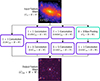 |
Fig. B.2. Inception block used in our full network architecture, Figure B.1. The block is composed of convolutional layers (purple) and a max pooling layer (turquoise). The inception block uses a mix of 1 × 1, 3 × 3, and 5 × 5 convolution, all with same padding and a stride of one to maintain the input dimensions H × W. We show the number of channels as a fraction of the output number of channels as this is variable, as shown in Figure B.1. |
The inception block show in Figure B.2 uses several convolutional layers (purple) with different kernel sizes and a max pooling layer (turquoise) to extract features. The input to the inception block is the output from the previous layer in the network, or the input to the network, with the output from each layer shown under the layer name. The height and width of the input features remains unchanged, while the number of channels is a fraction of the output number of channels for that inception block. 1 × 1 convolutional layers help with reducing the number of channels before 3 × 3 and 5 × 5 convolutional layers, reducing the computational cost, while a mix of max pooling and different sized convolutional kernels can learn different spatial features over different receptive fields.
Appendix C: Training choices
To evaluate the best hyperparameters for training, we perform several tests. We used the reduced architecture as this enables faster testing and trained the NN ten times for 150 epochs for each test case to use ensemble learning, reducing training stochasticity. We train the network on the total mass maps with the BAHAMAS simulations, with all simulations treated as known, unless otherwise stated. Each trained NN will generate a set of estimations for each simulation that we can treat as a posterior, then using ensemble learning, we multiply the posteriors of the ten NNs for the same test case to get a final posterior. From the final posterior, we take the median and quantiles representing 1σ and 2σ.
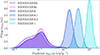 |
Fig. C.1. Trained ensemble of ten clustering NNs after calibration on all BAHAMAS simulations, all treated as known. We show the combined PDF of log(σDM/m) for the ten NNs with all simulations within 1σ of their target σDM/m except BAHAMAS-0.1 which is within 2σ. |
The configuration found to give the best accuracies and Gaussian like posteriors is when σDM/m is logarithmically transformed, all CDM simulations are treated as known and assigned the same effective σ of BAHAMAS-CDM, and X-ray maps are excluded. For this configurations, all BAHAMAS simulations are < 1σ of their target σDM/m except BAHAMAS-0.1 which is < 2σ. Figure C.1 shows the estimated σDM/m posteriors for each simulation with all simulations having Gaussian like posteriors except BAHAMAS-CDM which are asymmetric. The following subsections will justify each choice made.
Appendix D: Interpreting latent dimensions
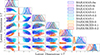 |
Fig. D.1. 7D latent space from a NN using the full architecture trained on all BAHAMAS and DARKSKIES simulations, with all simulations treated as known and X-ray maps included. The diagonal subplots show the distribution of values from each simulation in each dimension, while the off-diagonal show the correlation between each dimension pair. The NN was trained with an information-ordered bottleneck, resulting in the last dimensions (right-most columns and bottom-most rows) being biased towards containing the least important information. The first dimension is enforced to correspond to σDM/m via Equation 3. The first three dimensions show the majority of the physical information, showing σDM/m, the level of AGN feedback, and the separation of BAHAMAS from DARKSKIES, while the later dimensions are modifications of the earlier dimensions, structure dimensions to enable simulations forced apart in other dimensions to be brought closer globally, or Gaussian-like dimensions where little information is encoded. |
In Figure D.1, we show the full 7D latent space from a NN using the full architecture trained for 150 epochs on all BAHAMAS and DARKSKIES simulations with all treated as known. We include X-rays maps to show the more expressive latent space showing the difference between BAHAMAS-0w and BAHAMAS-0s. The diagonals show the distribution of each simulation, normalised to a peak of one for easier visualisation, in each dimension. The off-diagonals represent the correlations between latent dimensions for each simulation, here we can more easily see structure and how different learned features are expressed. The left-most column and top row corresponds to the first dimension, with right increasing columns and down increasing rows representing higher dimensions. Due to the information-ordered bottleneck, as the dimension increases, it has a lower probability of carrying its information through to the loss function, and therefore, is biased towards representing less important features.
The first dimension (first column and row) is enforced to be σDM/m via the loss function from Equation 3; therefore, it is unsurprising that the simulations are ordered in increasing σDM/m. The second dimension (second column and row) primarily discriminates between DARKSKIES and BAHAMAS given by the minimal overlap between the two suites of simulations in this dimension. However, looking at the correlation plots between dimensions one to three, we see that these hold the main physical information of σDM/m and the level of AGN feedback, identified by the T shape, most prominent in the correlation between dimensions 1-3 and 2-3, with dimension three encoding both an increasing σDM/m and level of AGN feedback. Dimension five is the next dimension to show physical information encoded, with it being similar to the first; however with DARKSKIES offset from BAHAMAS. Finally dimension six is the last that can be physically interpreted with it discriminating between DARKSKIES and BAHAMAS, but to a weaker extent as dimension two. The remaining two dimensions, dimensions four and seven, do not encode any physical information. However, four can be interpreted as a structure dimension that can allow simulations forced far away in other dimensions to be brought closer in this dimension. Structure dimensions can help reduce opposing loss functions, such as the requirement from Equation 3 for BAHAMAS-1 to be far away from BAHAMAS-0 in dimension one, while the similarity between BAHAMAS-0 and BAHAMAS-1 from Equation 1 wanting to bring them closer together as the different in σDM/m only has a minor impact on galaxy clusters, where other effects such as the level of AGN feedback or simulation resolution can contribute more to the difference. Dimension seven, due to it being the last dimension, does not hold a lot of information and is closer to a Gaussian-like initialisation with only a minor separation between BAHAMAS and the strongest DARKSKIES.
The types of dimensions observed here are commonly reproduced by NNs trained with different combinations of data and hyperparameters, we generally see a primary dimension for each physical difference, such as σDM/m, AGN feedback, and simulation suite, with secondary dimensions representing these physical differences with slight perturbations. We also see the structure dimensions, followed by the remaining dimensions being Gaussian-like, depending on the number of latent dimensions and number of physical difference in the training data. In the future, we will add more suites of simulations, expanding the number of physical difference and hopefully producing a more interpretable feature space, while also investigating more quantitive methods for identifying what each latent dimension is learning.
All Tables
All Figures
|
Fig. 1. Architecture and loss functions used in this paper. The input is the total mass and optionally X-ray maps that is then compressed using a convolutional NN (blue encoder) into a 7D latent space. From this latent space, we can get the similarity cluster and distance losses, Equations 1 and 3, or further transform it using a fully connected NN (red classifier) to obtain the classification loss, Equation 2. All losses are then weighted summed using the weights λCCLP, λdist, and λclass, Equation 4. See Figure B.1 for the full encoder and classifier architecture. |
| In the text | |
|
Fig. 2. Average classification accuracy from five NNs, normalised to the asymptotic accuracy, against the number of latent dimensions. Two sets of NNs are trained, one with X-rays included (reds/triangles) and the other excluded (blues/non-triangles). Each line shows an increase in the number of simulations included in the training, starting with BAHAMAS-0 and BAHAMAS-SIDM (solid), then BAHAMAS-AGN (dashed), and finally DARKSKIES (dotted). We fitted each set of data with an y = a + arctan((|𝒵|−b)/c) fit (lines). |
| In the text | |
|
Fig. 3. First two components of the PCA of the 7D latent space. Each point corresponds to a galaxy cluster from its colour corresponding simulation with the contours representing the 68% region for that simulation. The unknown datasets, BAHAMAS-0w and BAHAMAS-0s, are represented by the hatched contours and asterisk next to the legend label. We interpret that the first component corresponds to a transformation of log(σDM/m) and the second component corresponds to the level of AGN feedback. |
| In the text | |
|
Fig. 4. Method of building confidence in our ML estimator for data outside the training domain. Left: Train ensemble of ten regression NNs on the fiducial hydro BAHAMAS simulations. We show the combined PDF of log(σDM/m) for the known BAHAMAS simulations (blue shades) and blind uniform random noise (hatched black). We find that the regressor consistently estimates a significant, positive cross-section of ∼0.6 cm2g−1 with no regard to its confidence, presenting the issue with direct regression estimators. Right: First and third latent dimensions from our compact clustering algorithm trained with the same fiducial BAHAMAS as known (blue shades) and the random noise dataset as unknown (hatched black). The first latent dimension corresponds to log σDM/m, which we would naively assume that the noise dataset has a cross-section of ∼0.1 cm2 g−1; however, from the third dimension we see that the noise dataset shares no similarities with the known simulations and therefore, cannot be trusted. |
| In the text | |
|
Fig. 5. Consistency check on in-distribution testing. Left: Trained ensemble of three clustering NNs and combined PDF of log(σDM/m) for the known BAHAMAS-0, BAHAMAS-0.3, and BAHAMAS-1 (solid blue shades) and unknown BAHAMAS-0.1 (dashed black). We find a cross-section of ∼0.05 cm2 g−1 and within 1σ of 0.1 cm2 g−1 for BAHAMAS-0.1. Right: Projected 7D latent space from our clustering algorithm into a 1D distance PDF, where each known simulation (blue shades) is projected in the direction from the centre of their distribution to the centre of BAHAMAS-0.1. BAHAMAS-0.1 (hatched black) is projected in the direction of BAHAMAS-0.3 to show the greatest overlap. The distance has arbitrary units as it depends on the scale of the latent space. BAHAMAS-0.1 shares a large overlap of 49% and 55% with BAHAMAS-0 and BAHAMAS-0.3, respectively, leading to the conclusion that it lies within the training domain. |
| In the text | |
|
Fig. 6. 7D latent space projection from our clustering algorithm into a 1D distance PDF, where each known simulation and BAHAMAS-0s is projected in the direction from the centre of their distribution to the centre of BAHAMAS-0w (blue shades and pink hatched). BAHAMAS-0w is projected in the direction of BAHAMAS-0 to show the greatest overlap (purple hatched). The distance has arbitrary units as it depends on the scale of the latent space. BAHAMAS-0w shares a large overlap with BAHAMAS-0, leading to the conclusion that it lies within the training domain. |
| In the text | |
|
Fig. 7. Adaptation to a new domain. Left: Train ensemble of five clustering NNs with BAHAMAS, DARKSKIES-0, and DARKSKIES-0.2 as known (solid blue and red shades) and DARKSKIES-0.1 as unknown (hatched black). We show the combined PDF of log(σDM/m) from the five runs. We find a cross-section of ∼0.14 cm2 g−1 for DARKSKIES-0.1, within 1σ of 0.1 cm2 g−1. Right: Overlap confidence (left axis, solid blue), estimated σDM/m (right axis, dashed purple), and target σDM/m (right axis, dotted black) for DARKSKIES-0.1 as we progressively add known simulations during training. We start with BAHAMAS-0 and BAHAMAS-SIDM, then add the BAHAMAS-AGN simulations, DARKSKIES-0, and finally DARKSKIES-0.2. We see that the overlap confidence closely follows the convergence of DARKSKIES-0.1 onto the target σDM/m with an overlap of 70% resulting in DARKSKIES-0.1 being within 1σ of the target σDM/m. |
| In the text | |
|
Fig. B.1. Full network architecture used in the paper. The network is composed of inception blocks (purple, rounded rectangles), show in Figure B.2, max pooling layers (turquoise, trapeziums), linear layers (red, rectangles), a flatten layer (yellow, rectangle), and an information-ordered bottleneck layer (yellow, rounded rectangle). The output dimensions of each layer is represented underneath the name of the layer, the arrows represent the direction of data flow and if there is a ×2 next to the arrow, then the layer is repeated twice. The input is the total mass maps and optionally X-ray maps of galaxy clusters and the latent space is where we calculate the loss functions from equations 1 and 3 as well as our feature analysis. |
| In the text | |
|
Fig. B.2. Inception block used in our full network architecture, Figure B.1. The block is composed of convolutional layers (purple) and a max pooling layer (turquoise). The inception block uses a mix of 1 × 1, 3 × 3, and 5 × 5 convolution, all with same padding and a stride of one to maintain the input dimensions H × W. We show the number of channels as a fraction of the output number of channels as this is variable, as shown in Figure B.1. |
| In the text | |
|
Fig. C.1. Trained ensemble of ten clustering NNs after calibration on all BAHAMAS simulations, all treated as known. We show the combined PDF of log(σDM/m) for the ten NNs with all simulations within 1σ of their target σDM/m except BAHAMAS-0.1 which is within 2σ. |
| In the text | |
|
Fig. D.1. 7D latent space from a NN using the full architecture trained on all BAHAMAS and DARKSKIES simulations, with all simulations treated as known and X-ray maps included. The diagonal subplots show the distribution of values from each simulation in each dimension, while the off-diagonal show the correlation between each dimension pair. The NN was trained with an information-ordered bottleneck, resulting in the last dimensions (right-most columns and bottom-most rows) being biased towards containing the least important information. The first dimension is enforced to correspond to σDM/m via Equation 3. The first three dimensions show the majority of the physical information, showing σDM/m, the level of AGN feedback, and the separation of BAHAMAS from DARKSKIES, while the later dimensions are modifications of the earlier dimensions, structure dimensions to enable simulations forced apart in other dimensions to be brought closer globally, or Gaussian-like dimensions where little information is encoded. |
| In the text | |
Current usage metrics show cumulative count of Article Views (full-text article views including HTML views, PDF and ePub downloads, according to the available data) and Abstracts Views on Vision4Press platform.
Data correspond to usage on the plateform after 2015. The current usage metrics is available 48-96 hours after online publication and is updated daily on week days.
Initial download of the metrics may take a while.