| Issue |
A&A
Volume 705, January 2026
|
|
|---|---|---|
| Article Number | A186 | |
| Number of page(s) | 16 | |
| Section | Stellar structure and evolution | |
| DOI | https://doi.org/10.1051/0004-6361/202556724 | |
| Published online | 20 January 2026 | |
The light curve model fitting of Large Magellanic Cloud Cepheids: MESA-RSP versus Stellingwerf’s code predictions
1
INAF-Osservatorio astronomico di Capodimonte Via Moiariello 16 I-80131 Napoli, Italy
2
INAF-Osservatorio Astronomico d’Abruzzo Via Maggini sn 64100 Teramo, Italy
3
Istituto Nazionale di Fisica Nucleare (INFN)–Sez. di Napoli, Compl. Univ. di Monte S. Angelo, Edificio G Via Cinthia I-80126 Napoli, Italy
4
Inter-University Centre for Astronomy and Astrophysics (IUCAA) Post Bag 4 Ganeshkhind Pune 411 007, India
5
Department of Physics, Cotton University, Panbazar Guwahati 781001 Assam, India
6
European Southern Observatory Karl-Schwarzschild-Strasse 2 85748 Garching bei München, Germany
7
Scuola Superiore Meridionale Largo San Marcellino10 I-80138 Napoli, Italy
8
Department of Physics, State University of New York Oswego NY 23126, USA
★ Corresponding author: This email address is being protected from spambots. You need JavaScript enabled to view it.
Received:
2
August
2025
Accepted:
26
October
2025
Abstract
Context. A major challenge in modeling classical Cepheids is the treatment of convection, particularly its complex interplay with pulsation. This inherently three-dimensional (3D) process is typically approximated in one-dimensional (1D) hydrocodes, using dimensionless turbulent convection (TC) free parameters. Calibrating these parameters is essential for reproducing key observational features, such as the light curve amplitudes, secondary bumps, and the red edge of the instability strip (IS).
Aims. In this work, we calibrate the TC parameters adopted from the publicly available Modules for Experiments in Stellar Astrophysics-Radial Stellar Pulsations (MESA-RSP) code. We carried out a comparison using both the observational data of classical Cepheids and stellar parameter constraints from the Stellingwerf code. This is one of the few codes currently available that are capable of replicating a wide range of observed features of the classical pulsators.
Methods. We computed the multiband (V, I, and Ks) MESA-RSP light curves for 18 observed Large Magellanic Cloud (LMC) Cepheids, using stellar parameters determined on the basis of Stellingwerf’s code. By fine-tuning the mixing-length and eddy viscosity parameters, we calibrated the TC treatment in MESA-RSP. We compared the resulting period-luminosity (PL), period-radius (PR), and period-mass-radius (PMR) relations with the prediction of Stellingwerf’s model.
Results. We successfully reproduced the multiband (V, I, and Ks) light curves for 18 observed LMC Cepheids using the stellar parameters determined with Stellingwerf’s code. We also finetuned the mixing-length and eddy viscosity parameters in MESA-RSP. Our models yielded PL, PR, and PMR relations that were consistent with the previous results. Interestingly, although our results are broadly in agreement with previous works, we explicitly identified distinct mass-luminosity (ML) relations for fundamental-mode (FU) and first-overtone (FO) Cepheids for the first time. This suggests that the macroscopic phenomena affecting the ML relation depend on the stellar mass itself and/or on the effective temperature range. Our investigation is focused on the calibration of the TC parameters, but we did not find a single set of convective parameter values that was sufficient to reproduce all the light curves. In addition, no statistically significant correlation was found between the stellar properties (e.g., the effectives temperature or the stellar mass) and the convection parameters, although subtle trends for the period and effective temperature have been noted. As for the inferred Cepheid distances, our application of the model-fitting technique yields reddened distance moduli, in good agreement with those reported in previous works. This result is not surprising, given that we adopted the same input stellar parameters, with only minor differences in the adopted model atmospheres.
Key words: stars: distances / stars: fundamental parameters / stars: variables: Cepheids
© The Authors 2026
 Open Access article, published by EDP Sciences, under the terms of the Creative Commons Attribution License (https://creativecommons.org/licenses/by/4.0), which permits unrestricted use, distribution, and reproduction in any medium, provided the original work is properly cited.
This article is published in open access under the Subscribe to Open model. This email address is being protected from spambots. You need JavaScript enabled to view it. to support open access publication.
1. Introduction
Classical Cepheids (hereafter, Cepheids) are a class of intermediate-mass evolved (∼3 − 13 M⊙) pulsating stars crossing the instability strip during the core helium-burning phase (Bono et al. 2000; Anderson et al. 2016; Espinoza-Arancibia et al. 2022; Musella 2022). They are particularly renowned for their well-defined period-luminosity (PL) relation, which allows them to serve as excellent distance indicators (Leavitt 1908; Leavitt & Pickering 1912; Riess et al. 2022). Beyond their critical role in distance measurement, Cepheids also serve as ideal stellar laboratories for testing and validating stellar structure, evolution, and pulsation (e.g., Cassisi & Salaris 2011; Prada Moroni et al. 2012; Deka et al. 2025). Their pulsations provide additional insights into their stellar properties through detailed comparisons between theoretical predictions and observational characteristics, which also make them key tracers of stellar populations (Bono et al. 2005; De Somma et al. 2021). However, the reliability of stellar models depends heavily on the accuracy of the adopted input micro- and macro-physics (De Somma et al. 2024).
Cepheids occupy the classical instability strip (IS) of the Hertzsprung–Russell diagram (HRD), alongside other classical pulsators such as RR Lyrae stars, Type II and Anomalous Cepheids, and δ Scuti and SX Phoenicis stars. These stars exhibit periodic variabilities caused by regular changes in radius and luminosity, driven by temperature-dependent fluctuations in the gas opacity (Cox 1974). Their pulsations are mainly sustained by the κ-mechanism, with the γ-mechanism amplifying the driving process (Catelan & Smith 2015). The blue edge of the instability strip is related to the depth of the ionizing regions of the most abundant elements in the stellar envelope. In contrast, the occurrence of a red edge is due to the quenching action performed by convection on pulsation toward the redder zone of the color-magnitude diagram (CMD). However, the coupling between convection and pulsation not only affects the location of the red edge, but it also modifies the pulsation amplitudes and the capability of models to reproduce the observed light and radial velocity variations in detail (see e.g., Marconi et al. 2013, 2017; Bhardwaj et al. 2017; Paxton et al. 2019; De Somma et al. 2020, 2022). Besides radiation, convection is a key mechanism for transporting energy and momentum, as well as mixing elements within stars. Thus, it plays a significant role in shaping the stellar internal structure, evolution, and pulsation stability of stars. Given the extremely large scale of stars and their high viscosity, convection in stars typically occurs at extremely high Reynolds numbers1. As a result, stellar convection is predominantly characterized by a fully developed turbulent state. The theory of turbulent convection has been developed over the past 100 years, however, due to computational limitations, it remains challenging to establish a comprehensive theory that is fully able to explain the nature of convection in stellar models. Meakin (2008) estimated that a completely resolved simulation of stellar turbulence would require at least ∼60 years, based on computing trends available at the time and under the assumption that Moore’s law would continue to hold. As a consequence, turbulent convection, which is an inherently three-dimensional (3D) phenomenon, has been incorporated in one-dimensional (1D) codes based on simplified theoretical considerations. This involves several dimensionless free parameters, also known as turbulent convection (TC) free parameters.
To study the stellar interior structure and the different evolutionary phases, stellar models still heavily rely on the steady-state 1D convective formulation, namely, the so-called mixing length theory (MLT; Böhm-Vitense 1958; Henyey et al. 1965). There have been some recent additions in this regard, such as the turbulent convection model by Kuhfuss (1986), Kuhfuß (1987). The MLT approach is only suitable for calculating the stellar structure and quasi-static evolution of a star, as the timescale of stellar evolution is much longer than the timescale of the stellar convective motion. We need a time-dependent nonlocal theory of convection to study stellar pulsations, as the timescales of pulsation and convection are on the same order as that of the magnitude.
As mentioned above, in classical pulsators with relatively cool effective temperatures, convection plays an important role; however, this is not the case for the entire envelope, but in the ionization zones specifically. These are regions of instability mechanisms, where steep temperature gradients are present. When this region becomes convectively unstable, energy is transported by convection more efficiently. Furthermore, during pulsation, the ionization fronts move back and forth, and the interaction between convection and pulsation becomes crucial in exciting and (most importantly) damping the pulsations. In addition, since this region is unstable, the behaviour of convection becomes more complex than in other environments. The importance of including convection in pulsation models has been highlighted in multiple studies (e.g., Gehmeyr 1992b; Feuchtinger 1999; Marconi 2009). In particular, for reproducing the observed red edge of the IS, the amplitude, and the secondary features of the light curves, nonlinear convective pulsation models are required. Several nonlinear convective pulsation codes have been developed in recent decades, which include a nonlocal time-dependent treatment of convection (see e.g., Stellingwerf 1982; Gehmeyr 1992a; Bono et al. 1999; Feuchtinger 1999; Kolláth et al. 2002; Marconi et al. 2005; Smolec & Moskalik 2008, and references therein).
Early hydrodynamical studies with the Florida-Budapest code highlighted the importance of turbulent convection in shaping pulsation dynamics. Kolláth et al. (2002) showed that double-mode behavior in Cepheids arises naturally when turbulent convection is included in their hydrodynamic model (i.e., the Florida-Budapest code). However, Smolec (2008) later argued that this behavior is actually a consequence of neglecting negative buoyancy in their pulsation code. The Cepheid phase lags were subsequently revisited by Szabó et al. (2007), also using the Florida-Budapest code. Kolláth et al. (2011) investigated period doubling in RR Lyrae models for the first time, providing the theoretical basis for its later detection in Blazhko RR Lyrae stars by Kepler. This framework was further supported by Smolec & Moskalik (2012) through their study of BL Herculis stars. Extending this line of work, Smolec & Moskalik (2012, 2014) explored variations of the “canonical” parameter sets in Type II Cepheid models and uncovered a range of dynamical phenomena, including period doubling, amplitude modulations, beat pulsations, and even chaotic variability behaviors. These works were motivated by Kolláth et al. (2011), who first demonstrated period doubling in RR Lyrae models after fine-tuning the α parameters in the Florida-Budapest code.
Building on this foundation, recent efforts with Modules for Experiments in Stellar Astrophysics-Radial Stellar Pulsations (MESA-RSP; Paxton et al. 2010, 2013, 2015, 2018, 2019; Jermyn et al. 2023) have been aimed at calibrating turbulent convection (TC) parameters against observations. For RR Lyrae (both fundamental RRab and first-overtone RRc) stars, Kovács et al. (2023, 2024) successfully reproduced radial velocity curves; however, matching detailed light curve morphologies remains a challenge. This discrepancy suggests the need for either refined calibration or improved convection modeling. In the case of Cepheids, the effects of various control parameters in MESA on Cepheid evolutionary tracks were investigated in great detail by Ziółkowska et al. (2024). Recent studies by (Kurbah et al. 2023; Kovács et al. 2023, 2024; Das et al. 2025) suggest that the turbulent parameter prescriptions require rigorous calibration with observational data to simultaneously reproduce the observed light and radial velocity curve morphologies; particularly with respect to the amplitude and the secondary features (e.g., bumps) in the light curves. However, it is important to note that these parameters do not significantly affect the mean magnitudes, mean PL relation, or topology of the IS edges (De Somma et al. 2022; Deka et al. 2024; Das et al. 2024). Interestingly, Deka et al. (2024) found that some models pulsate beyond the estimated traditional linear red edge, which could arise due to an uncalibrated TC parameter set. Alternatively, it could indicate that such pulsators genuinely exist but have not been observed due to their relatively short lifespan. Before drawing any conclusions, further tests are needed.
In this work, we aim to calibrate the free convective parameters adopted in the MESA-RSP code against observational data for Cepheid variables. To do so, we selected several observed Cepheids that have already been precisely modeled using Stellingwerf’s code with their stellar parameters published in Ragosta et al. (2019; hereafter R19). Given the large number of free parameters involved in the MESA-RSP tool, we adopted this approach to reduce the number of unknowns in our TC parameter calibration process.
The remainder of the paper is organized as follows. In Section 2, we provide a brief comparative overview of the Stellingwerf and MESA-RSP codes. Section 3 presents the data and methodology used in this work. The results, along with a discussion of the effects of the TC parameters on the light curves, are presented in Section 4. Finally, Section 5 outlines our findings and future prospects.
2. MESA-RSP versus Stellingwerf code
Both MESA-RSP and Stellingwerf’s codes are nonlinear convective pulsation hydrocodes that couple convection with the equations of radiation hydrodynamics through an additional equation for turbulent energy. However, the mathematical formulation of MESA-RSP particularly in its treatment of convection, differs from that of Stellingwerf’s code (see below for the details of the parameters). Therefore, a one-to-one calibration of the TC parameters is not possible. A practical and reliable approach in calibrating both codes is to match them against the same observed stellar properties using identical input stellar parameters. In addition, a detailed analysis of the temporal and spatial behavior of turbulent energy can offer further insights into the weaknesses and strengths of the underlying turbulent energy equations. Such a comparative study, focused exclusively on the temporal and spatial characteristics of the turbulent energy equations in both Stellingwerf’s code and Kuhfuss (1986), has already been carried out by Gehmeyr & Winkler (1992). Although the models developed by Kuhfuss (1986) and Stellingwerf remain among the most widely used for simulating the observations of the variable stars, the literature still lacks a thorough quantitative comparison of the dimensionless convective parameters involved in these two codes.
Recently, MESA-RSP was made publicly available, enabling us to model linear and nonlinear radial pulsations exhibited by variable stars such as classical and Type II Cepheids and RR Lyraes (Smolec & Moskalik 2008; Paxton et al. 2019). It implements the time-dependent turbulent convection model of Kuhfuss (1986), following the stellar pulsation framework described in Smolec & Moskalik (2008). This convection model incorporates eight free dimensionless parameters:
-
α
(Mixing length): distance a convective element travels before dissipating;
-
αm
(Eddy viscosity): effective viscosity from turbulent momentum transport;
-
αs
(Turbulence source): turbulence generation via shear, buoyancy, or forcing;
-
αc
(Convective transport): efficiency of energy transport by convection;
-
αd
(Turbulence dissipation): conversion of turbulent energy into heat;
-
αp
(Turbulent pressure): pressure contribution from turbulent motion;
-
αt
(Turbulent flux): transport of mass, momentum, and energy by turbulence;
-
γr
(Radiative losses): energy lost from convective eddies via radiation.
Four different combinations of these parameters are given in Paxton et al. (2019), labeled as A, B, C, and D. In set A, turbulent pressure, turbulent flux, and radiative cooling are neglected (i.e., αp = αt = γr = 0) and values of αs, αc and αd are kept the same as in Table A.1. Under this condition, the time-independent version of the Kuhfuss (1986) model becomes locally equivalent to the standard MLT (Böhm-Vitense 1958). Set B adds radiative cooling. This parameter was not present in the original Kuhfuss (1986) model; thus, it was set to  following Wuchterl & Feuchtinger (1998). Set C adds turbulent pressure (αp) and convective flux (αc ≡ αs) (Yecko et al. 1998). The αp parameter was implicitly included in the Kuhfuss (1986) model through turbulent convection, and thus turbulent pressure, but it had a fixed value of
  . Yecko et al. (1998) extended the model by allowing αp to be scaled. The αc parameter, which was not present in the original Kuhfuss (1986) model, was also introduced by Yecko et al. (1998). Set D includes all these effects simultaneously (Paxton et al. 2019). Parameter values follow those given in Tables 3 and 4 of Paxton et al. (2019), which are also summarized in Table A.1 in Appendix A of the present paper. For a more detailed discussion on these parameters, we refer to Kuhfuss (1986), Wuchterl & Feuchtinger (1998), Yecko et al. (1998), Smolec & Moskalik (2008).
The original version of Stellingwerf’s code was developed by Stellingwerf (1982) based on the unpublished work of Castor (1968) and it was later improved by Bono & Stellingwerf (1994), Bono et al. (1999), De Somma et al. (2024). The model includes a free convective parameter (analogous to the α’s in MESA-RSP) proportional to the ratio between the mixing length, λ, that is the path covered by the convective elements and the pressure height scale. This parameter in Stellingwerf’s code is used to close the nonlinear equation system. Another free parameter is either set as the eddy-viscosity dissipation parameter or eddy-viscosity mean free path. Both the turbulent pressure and the eddy viscosity pressure (ignoring a constant of order unity) form one component of a nine-component symmetric tensor (Reynolds stress tensor). The third free parameter is the turbulent diffusion parameter, λovs. Although the relations between these parameters have not been studied in detail through comparisons between theoretical observables and observational constraints, λev and λovs values are typically chosen such that λev ≈ λ and λovs ≈ λ/10; reducing the number of free parameters that need to be calibrated. For a detailed description, we refer to Bono & Stellingwerf (1994).
3. Data and methodology
3.1. The sample and the selected input model parameters
We selected 18 Large Magellanic Cloud (LMC) Cepheids from R19, consisting of 11 fundamental (FU) and 7 first-overtone (FO) mode Cepheids. The periods of these Cepheids span a wide range of approximately 1 to 30 days. This sample also spans a wide range of luminosities and light curve shapes. The stellar parameters required for pulsation model computations are mass (M), luminosity (L), effective temperature (Teff), and chemical composition (X, Y, and Z), which were also taken from R19. Additionally, we adopted the mixing-length efficiency parameter (α), one of the TC parameters, from this paper as our starting point. The list of parameters is reported in Table 1, whereas the positions of these Cepheids in the HRD are shown in Fig. 1.
List of Cepheids analyzed in this work.
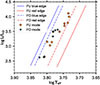 |
Fig. 1. Location of the Cepheids selected in this work on the HRD. The IS edges are taken from Deka et al. (2024). |
We used multifilter light curves in the V, I, and the Visible and Infrared Survey Telescope for Astronomy (VISTA) Ks-bands of the selected Cepheids to calibrate the TC parameters. The observed optical V- and I-band light curves were obtained from the Optical Gravitational Lensing Experiment (OGLE)-IV database2 (Soszyński et al. 2015). The near-infrared Ks-band light curves were sourced from the “VISTA near-infrared Y, J, Ks survey of the Magellanic Clouds system” (VMC) survey (Cioni et al. 2011; Ripepi et al. 2016, 2017, 2022).
In MESA-RSP, there are four different combinations of the eight free TC parameters, which are considered fiducial and have not been calibrated to observations. For the initial computation, we set the mixing-length efficiency parameter as given in R19, while the remaining seven parameters (αm, αc, αs, αd, αp, αt, and γr) are described in Table A.1. MESA-RSP solves the pulsation equations using a Lagrangian mesh, structured into inner and outer zones, based on a specified anchor temperature, which we set to Tanchor = 11 000 K. Initially, the total number of Lagrangian mass cells was set to Ntotal = 200, with Nouter = 60 cells above the anchor. However, if this configuration failed to generate the initial model, we adjusted the setup to Ntotal = 150 and Nouter = 40. The selection of numerical parameters, including the inner boundary temperature (Tinner = 2 × 10⁶ K), follows the guidelines as outlined in Paxton et al. (2019) (for further details, see Appendix B of Deka et al. (2024)). These parameters remained fixed throughout the entire calibration process.
To perturb the initial model, we set the surface velocity parameter, RSP_kick_vsurf_km_per_sec, to 0.1. For mode selection, RSP_fraction_1st_overtone was set to 0 for FU mode and 1 for FO mode. The RSP_fraction_2nd_overtone was set to 0 in all cases, as our sample consists exclusively of FU and FO Cepheids. If we were unable to obtain the desired pulsation mode for a particular star, we systematically adjusted the RSP_kick_vsurf_km_per_sec parameter (discussed in more detail in Sect. 3.3)3. Such difficulties typically arise in the hysteresis domain, where the resulting mode depends sensitively on the initial conditions (Kolláth et al. 2002; Smolec & Moskalik 2010).
We considered the model to have reached full-amplitude stable mode when the pulsation period, P, the fractional growth of the kinetic energy per pulsation period, and the amplitude of radius variation ΔR do not differ by more than ∼0.0001 over the last ∼100-cycles of the total integrations computed. It takes ∼1000 − 4000 pulsation cycles to reach full-amplitude stable mode pulsations for these models.
3.2. Conversion of bolometric light curves to the V, I, and Ks filters
Pulsation codes typically output bolometric light curves that need to be converted into observational photometric systems to allow for a direct comparison with the observed curves. While the most rigorous approach involves solving the radiative transfer equation (accounting for local thermodynamic equilibrium (LTE) or non-LTE (NLTE) effects) to compute filter-specific magnitudes, this is computationally expensive. For practical applications, pre-computed bolometric correction (BC) tables offer an efficient alternative. In this work, we use MESA’s built-in interpolation routines to extract BCs as a function of stellar parameters (e.g., Teff, log g, [Fe/H]) at each pulsation phase. We applied BCs to all phases of the light curve to account for depth differences across different pulsation cycles.
We adopted the BC tables from Lejeune et al. (1998) for optical bands V and I. For the Ks-band, we used the BC tables from the MESA Isochrones & Stellar Tracks (MIST) model grids (Choi et al. 2016; Dotter 2016)4, which are derived from the C3K grid (Conroy et al., in prep.). The C3K grid employs 1D atmospheric models based on ATLAS12/SYNTHE (Kurucz 1970, 1993).
3.3. TC parameter calibration
We computed models for each target using four distinct combinations of fiducial TC parameters (sets A, B, C, and D). For each target, we selected the best-fitting model and then refined it by varying either α or αm in small steps of 0.1 and 0.01, respectively, either increasing or decreasing them as needed to match the observed amplitudes. It should be noted that α and αm are not entirely independent: changing α also affects αm through the underlying convection equations. This has been discussed in detail in Kolláth et al. (2002). This interdependence is typical of most 1D pulsation codes.
The surface velocity parameter, RSP_kick_vsurf_km_per_sec, was set to 0.1 (same as the MESA-RSP fiducial parameter) in most cases. However, in instances where the initial setting did not produce the desired pulsation mode, we adjusted this parameter in steps of 0.5. Additionally, in a few cases where the model period differed significantly from the observed period, we made slight modifications to L and Teff. For each target, we computed approximately 50 models (up to 100 in some cases) and identified the best-matched model using the model-fitting technique described in the next section. An example of all possible models for a Cepheid with the best fitted one is shown in Fig. 2.
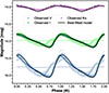 |
Fig. 2. Observed light curves (data points) for OGLE-LMC-CEP-1124 star is shown along with the best-fitting model predictions overlaid on all the computed models for this star. The χ2 values of the models range from 1.3 (best-fit model) to 49.4 (worst-fit model). |
3.4. Best-fit model estimation
The best-fit model was determined using a model-fitting technique following Marconi et al. (2017), Ragosta et al. (2019). Its implementation is detailed in the subsections below.
3.4.1. Light curve phasing
First, the observed light curves were phased using
 (1)
(1)
where t0 is the epoch of maximum light in the V-band, P is the pulsation period (in days), and t denotes the observation times. Both the theoretical and observed light curves (V, I, and Ks bands) were then phase-aligned, so that that maximum brightness would correspond to phase zero.
3.4.2. Interpolation and χ2 minimization
The theoretical light curves were interpolated to match the observed phases using a cubic spline (implemented via Python’s scipy.interpolate). The χ2 function, defined as
![Mathematical equation: $$ \begin{aligned} \chi ^2 = \frac{1}{N_{\rm {bands}}}\sum _{i = 1}^{N_{\text{bands}}} \frac{1}{N^{j}_{DOF}} \sum _{j = 1}^{N_{\text{points}}}\frac{\left[ m_j^i - \left( M_{\text{model}}^i (\phi _j^i + \delta \phi ^i) + \delta M^i \right) \right]^2}{\sigma ^j_i}, \end{aligned} $$](/articles/aa/full_html/2026/01/aa56724-25/aa56724-25-eq4.gif) (2)
(2)
was minimized using the L-BFGS-B optimizer5 (Byrd et al. 1995). Here, we have
-
i: band index (V, I, Ks);
-
j: data point index;
-
Nbands: number of bands;
-
 : Npoints − 2; number of degrees of freedom;
 -
δMi: magnitude shift/distance modulus for ith band;
-
δϕi: phase shift between model and observed light curves;
-
Mmodel, m: model and observed apparent magnitudes, respectively;
-
 : observational uncertainty.
3.4.3. Bayesian refinement
The L-BFGS-derived parameters (δMi, δϕi) and their uncertainties were further refined through Markov chain Monte Carlo (MCMC) analysis using the EMCEE Python package (Foreman-Mackey et al. 2013). We used 32 walkers, 10 000 iterations, and 2000 burn-ins for the MCMC sampling.
4. Results and discussion
4.1. Light curve with MESA-RSP fiducial TC parameters
We initially computed a set of models for each target by setting one of the eight TC parameters in MESA-RSP, α, to the same value as given by R19, while keeping the remaining seven parameters at their fiducial values as defined in Paxton et al. (2019). We found that sets A and B produced nearly identical results in terms of morphological features. However, the models from set A yielded periods and amplitudes much closer to the observed values than those from set B. Similarly, sets C and D provided comparable results. In some cases, observations were better matched with models from set C or set D, rather than from sets A or B. The Teff of the stars played a crucial role in determining the best-matching set. Specifically, stars with Teff > 6000 K were better matched with set A models, whereas those with Teff < 6000 K showed better agreement with either set C or set D. This is expected as the convection efficiency increases toward the red edge (lower temperature). Furthermore, for some stars, we were initially unable to obtain the desired pulsation modes using the fiducial parameter settings. However, after adjusting the surface velocity parameter and keeping other parameters fixed, we successfully obtained the desired pulsation mode for these stars. Overall, 11 stars are best matched with set A, 1 with set C, and 6 with set D using the fiducial parameters based on the morphological structure, but not the amplitudes.
4.2. Best-fit models
The morphology of the MESA-RSP model with the fiducial TC parameters shows good agreement with the observed light curves both in terms of shape and the positioning of small bumps. However, the model amplitudes vary from approximately half to twice the measured amplitude and need to be matched. To achieve this, we varied the parameters α and αm individually to adjust the amplitudes in accordance with the observations. Additionally, we obtained the best-fit parameters (Δϕ and Δm), along with their associated uncertainties using the model-fitting technique described in Sect. 3. The observed light curves along with the best-matched models and for a subset of Cepheids with Stellingwerf’s best-fit curves, are shown in Figs. 3 and 4, respectively. We find a very good global agreement between the theoretical curves produced with MESA-RSP and Stellingwerf’s code. Fig. B.1 shows a representative posterior distribution from the Bayesian refinement analysis for the star OGLE-LMC-CEP-1124, demonstrating the parameter covariances and final uncertainty estimates. The best-fit parameters (stellar parameters and TC parameters) are summarized in Table C.1. In Fig. 5, we present the visual (top left panel), the I band (top right panel) and the unreddened (bottom left panel) distance modulii together with the radii (bottom right panel) derived in this work for each star, alongside the corresponding values from R19 for comparison. The radii show good agreement with those reported by R19. However, we observe subtle differences in the distance moduli for some stars. This small difference is likely due to differences in the bolometric corrections and color-temperature transformations or the methods employed to perform these conversions. Despite the consistency in the underlying models, this highlights that the choice of model atmospheres and their interpolation can have a significant impact on the derived distances. The phase shifts were found to range from approximately −0.02 and 0.08.
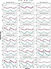 |
Fig. 3. Observed light curves (data points) for the selected Cepheids with the best-fitting model predictions overplotted as continuous lines. |
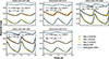 |
Fig. 4. Observed light curves (data points) for five selected Cepheids with the best-fitting model predictions from MESA-RSP and Stellinwerf code overplotted as continuous lines. |
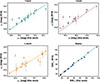 |
Fig. 5. Comparison between the reddened distance moduli (in the V, I, and Ks bands) and stellar radii derived in this work with those reported by R19. Each panel shows the respective comparison, including the error bars on the distance moduli, showing the consistency and deviations across photometric bands and radius estimates. |
We obtained the highest number of observation-matched models from set A, where αp = αt = γr = 0. To further investigate the impact of including these parameters on those models, we increased αp in steps of 0.1 from 0.0 to 1.0, setting γr to either 0 or 1 and αt = 0.01. Here, we refer to this new set of models as the “set D equivalent”. Examples of these models, along with those from set A, are shown in Fig. D.1. These models also provided a good match with the observations; however, in order to reproduce the observed amplitudes, it was necessary to again tune either α or αm compared to the best-fit models from set A. This is because αp adjusts the turbulent pressure, which directly influences the work integral. At the same time, the work integral is affected by the eddy viscosity, which is scaled by αm. Therefore, both parameters must be adjusted together to keep the work integral unchanged. In general, scaling one alpha parameter will require a corresponding adjustment of the others. Furthermore, in most of the stars, αp could not be increased beyond 0.2. Higher values either resulted in negative growth rates or failed to reproduce the observed light curve morphology.
We also found it necessary to modify the surface velocity parameter, since the values used for set A did not yield the desired pulsation modes. We did manage to achieve a good match for nearly all the stars. In some models, the inclusion of these parameters improved the light curve morphology, resulting in a better agreement with observations. One such example is OGLE-LMC-CEP-3131 (see top-center-left panel of Fig. D.1). However, in some cases, the fit worsened. For instance, in OGLE-LMC-CEP-2944, although the overall match remained reasonable, the characteristic bump disappeared (see middle-right panel of Fig. D.1). Setting γr to 1 could reproduce a light curve identical to that of set A, but it changes both the amplitude and the morphology of the radial velocity curves. The best-fit parameters (stellar and TC parameters) for this set of TC parameters are summarized in Table D.1.
As discussed earlier in this paper, similar light curve shapes can be reproduced with different combinations of TC parameters, leading to some degeneracy in the model outputs. One way to help reduce this degeneracy is to include radial velocity data in the fitting process. While different parameter combinations such as mixing length and eddy viscosity, can produce comparable light curve amplitudes, they often lead to distinct radial velocity amplitudes. This occurs because the light curve amplitude primarily reflects temperature variations near the photosphere, whereas the radial velocity is governed by the dynamical response of the stellar envelope. For example, increasing the eddy viscosity can suppress the mechanical motion of the pulsation without significantly affecting the temperature contrast, allowing two models to produce similar light curves, while differing in terms of the radial velocity behavior. We note, however, that this effect is most relevant for V and bluer bands, which are sensitive to Teff variations, while infrared bands such as Ks are more sensitive to radius changes and therefore not entirely independent of the radial velocity data. Furthermore, as the 1D convection models rely on strong simplifications and artificial parameterizations, a parameter set that reproduces the observed light curve most closely may not necessarily be more physically accurate than another.
To illustrate this, we present a comparative analysis between the set D equivalent and the set A models. While the period, light curve morphology, and amplitude reveal a close match for most stars in our sample, we observed notable differences in the surface velocity amplitudes, as shown in Fig. D.2. However, we acknowledge that a more systematic investigation is required to quantify these effects more robustly and we plan to address this in a future study.
4.3. Correlation between TC parameters and stellar properties
To systematically investigate potential relationships between the TC parameters and global stellar properties, we performed a series of linear regressions between key quantities. We focused on two key TC parameters:  and αm, comparing them with the Teff, mass, luminosity, and pulsation period values. A few examples of these comparisons is presented in Fig. 6.
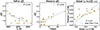 |
Fig. 6. Correlations between the stellar parameters and the TC parameters ( |


We find that the majority of parameter combinations show no strong or statistically robust correlations, with R2 values typically below 0.3. This suggests that neither  nor αm exhibits a strong linear dependence on the basic stellar parameters within our sample. The most notable exception is a moderate positive correlation between
  and both Teff and the pulsation period. The trend in temperature suggests that cooler stars tend to require higher convective efficiency, as expected and reported in previous literature (De Somma et al. 2022). Similarly, the trend with period may imply an indirect connection with stellar radius or evolutionary stage, as longer-period variables typically correspond to more evolved stars.
In contrast, correlations between αm and parameters such as Teff, mass, luminosity, and period are weak or statistically insignificant. However, for RR Lyrae stars, Kovács et al. (2023, 2024) reported a significant relationship between αm and Teff. The discrepancy between their findings and ours may stem from the degeneracy between αm and  . In their work,
  was held fixed, while αm was varied, whereas in our analysis,
  was set according to R19 (where it varies across stars), before adjusting αm to match the observed amplitudes. This methodological difference likely contributes to the weaker trends observed in our results. To explore this further, we examined the correlation between αm and
  , finding only a weak, scattered relationship (R2 = 0.029). While this suggests a possible empirical connection, the large intrinsic scatter points to substantial underlying variability. Additionally, the absence of stronger trends may partly reflect the limited sample size, which reduces the statistical power of our analysis. Another possibility is that such a correlation may not exist for Cepheids at all. This weaker parameter dependency could be due to their convective layers being more extended than in RR Lyrae stars. Future studies with larger samples and broader parameter coverage will be essential to clarify these relationships.
4.4. Stellar global parameter correlations
To quantify the pulsational properties of our model grid, we examined the relationships between key stellar parameters for both the FU and FO modes. In particular, we derived the period–radius (PR), period–mass-radius (PMR), and mass–luminosity (ML) relations shown in Fig. 7 as well as the PL relation in different bands shown in Fig. 8. Table 2 provides a detailed comparison between the theoretical relations derived in the current study and those previously established by R19.
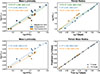 |
Fig. 7. ML, PR, and PMR relations derived from our best-fit model set. Two distinct relations for FU and FO cepheids are clearly distinct in each case. |
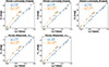 |
Fig. 8. PL and PW relations in the V, I, and Ks-bands derived from out best-fit model set. The relations are in very good agreement with that in R19. |
Comparison of the relations derived in this work with R19.
We did not observe any modifications in the masses and luminosities of the stars from those reported in R19. Additionally, the upper left panel of Fig. 7 suggests that FO Cepheids exhibit more canonical behavior (i.e., less convective overshooting) than FU Cepheids, particularly at higher masses. R19 established a single PR relation for both FU and FO Cepheids by fundamentalizing FO Cepheids. However, in this work, we derived two distinct relations for the two modes as shown in the upper right panel of Fig. 7. As expected, the PR relation from R19 aligns more closely with the FU relation derived in this study. Similarly, the PMR relation from R19 shows very good agreement with our FU-mode PMR relation.
Figure 8 presents the PL relations from our models in the V, I and Ks-bands as well as the Wesenheit indices. These relations also show excellent agreement with those from R19, with a comparable scatter.
5. Summary and conclusion
We selected a sample of 18 Cepheids, including 11 FU and 7 FO Cepheids in the LMC, which had previously been modeled by R19 using the Stellingwerf code. We obtained the light curve in the optical bands (V, I) from the OGLE IV database and the NIR light curve Ks band from the VMC survey. We adopted the stellar parameters (i.e., mass, luminosity, effective temperature, and chemical compositions) from R19 and calibrated the TC parameters (i.e., αMLT, αm, αp, and γr) to achieve the best agreement with the observed light curves. Our models successfully reproduced the observed light curves for all 18 stars in the sample, showing good agreement in magnitude shifts, radii, and phase alignment across multiple bands. The key findings of this study can be summarized as follows.
-
We achieved good agreement with observations for all 18 stars. The derived stellar parameters for the mass and luminosity are consistent with those reported in R19. However, for four stars, our models yield slightly different effective temperatures, with deviations ranging from approximately 20 to 250 K.
-
The morphology of the light curves was successfully reproduced with the fiducial TC parameters of MESA-RSP themselves. However, to achieve observation-consistent amplitude, we adjusted the mixing-length parameter (
 ) and eddy viscous dissipation parameter (αm). We find that most of the stars with Teff > 6000 K prefer the simplest convection theory, while stars with Teff < 6000 K require the inclusion of turbulent pressure (αp), turbulent flux (αt), and in some cases, radiative loss (γr). We conclude that the fiducial TC parameters of MESA-RSP are adequate for reproducing the general shape of light curves across the temperature range studied; however, parameter tuning is essential to accurately reproduce their observed amplitudes.
 -
We also tested the inclusion of the parameters αp, αt, and γr in models with Teff > 6000 K. We found that most stars favor a low value of αp (typically ∼0.2–0.5) and no radiative cooling (i.e., γr = 0). This could still lead to a degeneracy among the TC parameters when reproducing the observations. However, despite an excellent fit to the multiband light curves, noticeable differences in the radial velocity amplitude remain, which could provide a means to break this degeneracy.
-
We also found a good agreement in the multiband PL, PR, PMR, and ML relations with R19. However, we identified two distinct ML relations for FU and FO Cepheids that had not been previously reported. This finding suggests a possible dependence on macroscopic phenomena that influence the ML relation.
-
We did not find any statistically significant correlation between αMLT or αm and the stellar parameters. However, we did observe subtle trends between αMLT and αm with the pulsation period and Teff. We emphasize that before drawing any firm conclusions in this regard, a larger sample of observationally consistent models spanning the entire IS is required.
-
From this study, we also found that no single set of TC parameters can successfully model Cepheids across the entire IS. Even when restricting our analysis to observations from the central region of the IS, we observe that different combinations of TC parameters are required to reproduce the light curve features. This suggests that rather than relying on a universal parameter set, it might be more effective to establish empirical or semi-empirical relations between the TC parameters and the observable quantities. Such relations would significantly accelerate model computations and improve the efficiency of parameter space exploration. However, the number of observation-consistent models available at present is still statistically too small to robustly establish such relations.
In this work, we did not attempt to present a more physically motivated picture of Cepheids, nor do we claim that our models are more accurate in terms of stellar physics than those included in previous studies. Rather, our primary goal has been to reproduce the observed light curves and match the Stellingwerf models with MESA-RSP models, focusing on light curve morphology and amplitudes. Although MESA-RSP is more frequently adopted by the community (Das et al. 2021; Deka et al. 2022; Das et al. 2024, 2025; Kurbah et al. 2023; Hocdé et al. 2024; Espinoza-Arancibia & Pilecki 2025), there is still a lack of sufficient nonlinear models that successfully match observations. However, developing such observation-consistent models is essential for constraining the effects of TC parameters on light curve morphology and the physical characteristics of Cepheids. These models also make it possible to obtain more precise determinations of stellar parameters, which are critical for galactic archaeology. Additionally, they provide a foundation for calibrating 1D TC prescriptions using the results from 3D hydrodynamical simulations.
Thus far, our analysis has primarily focused on tuning the parameters α and αm to achieve the desired amplitudes. MESA-RSP performs quite well in reproducing the observed light curves of Cepheids without any significant modifications in the α parameters. However, a comprehensive investigation of the other α parameters is still required to fully understand their influence on the minute details of the light curves. Additionally, the effects of these parameters on the dynamics of inner zones and the transition region remain largely unexplored, not only in this work, but also in the existing literature. We plan to address these aspects in our future studies.
Acknowledgments
We thank the anonymous referee for the constructive and valuable feedback. MD acknowledges funding from the INAF 2023 Large Grant MOVIE (PI: Marcella Marconi) and project PRIN MUR 2022 (code 2022ARWP9C) “Early Formation and Evolution of Bulge and HalO (EFEBHO)”, PI: Marcella Marconi, funded by European Union – Next Generation EU. MD also acknowledges the use of the High-Performance Computing facility Pegasus at IUCAA, India. To compute the models, we used MESA r23.05.1 (Paxton et al. 2010, 2013, 2015, 2018, 2019). G.D.S. acknowledges funding from the INAF-ASTROFIT fellowship (PI: G. De Somma), from Gaia DPAC through INAF and ASI (PI: M.G. Lattanzi), and from INFN (Naples Section) through the QGSKY and Moonlight2 initiatives. AB thanks the funding from the Anusandhan National Research Foundation (ANRF) under the Prime Minister Early Career Research Grant scheme (ANRF/ECRG/2024/000675/PMS). This research was supported by the International Space Science Institute (ISSI) in Bern/Beijing through ISSI/ISSI-BJ International Team project ID #24-603 – “EXPANDING Universe” (EXploiting Precision AstroNomical Distance INdicators in the Gaia Universe).
References
- Anderson, R. I., Saio, H., Ekström, S., Georgy, C., & Meynet, G. 2016, A&A, 591, A8 [NASA ADS] [CrossRef] [EDP Sciences] [Google Scholar]
- Bhardwaj, A., Kanbur, S. M., Marconi, M., et al. 2017, MNRAS, 466, 2805 [NASA ADS] [CrossRef] [Google Scholar]
- Böhm-Vitense, E. 1958, Zap, 46, 108 [Google Scholar]
- Bono, G., & Stellingwerf, R. F. 1994, ApJS, 93, 233 [Google Scholar]
- Bono, G., Marconi, M., & Stellingwerf, R. F. 1999, ApJS, 122, 167 [NASA ADS] [CrossRef] [Google Scholar]
- Bono, G., Caputo, F., Cassisi, S., et al. 2000, ApJ, 543, 955 [NASA ADS] [CrossRef] [Google Scholar]
- Bono, G., Marconi, M., Cassisi, S., et al. 2005, ApJ, 621, 966 [NASA ADS] [CrossRef] [Google Scholar]
- Byrd, R., Lu, P., Nocedal, J., & Zhu, C. 1995, SIAM J. Sci. Comput., 16, 1190 [Google Scholar]
- Cassisi, S., & Salaris, M. 2011, ApJ, 728, L43 [NASA ADS] [CrossRef] [Google Scholar]
- Catelan, M., & Smith, H. A. 2015, Pulsating Stars (Germany: Wiley-VCH) [Google Scholar]
- Choi, J., Dotter, A., Conroy, C., et al. 2016, ApJ, 823, 102 [Google Scholar]
- Cioni, M. R. L., Clementini, G., Girardi, L., et al. 2011, A&A, 527, A116 [CrossRef] [EDP Sciences] [Google Scholar]
- Cox, J. P. 1974, Rep. Prog. Phys., 37, 563 [Google Scholar]
- Das, S., Kanbur, S. M., Smolec, R., et al. 2021, MNRAS, 501, 875 [Google Scholar]
- Das, S., Molnár, L., Kanbur, S. M., et al. 2024, A&A, 684, A170 [NASA ADS] [CrossRef] [EDP Sciences] [Google Scholar]
- Das, S., Molnár, L., Kovács, G. B., et al. 2025, A&A, 694, A255 [NASA ADS] [CrossRef] [EDP Sciences] [Google Scholar]
- De Somma, G., Marconi, M., Cassisi, S., et al. 2020, MNRAS, 496, 5039 [CrossRef] [Google Scholar]
- De Somma, G., Marconi, M., Cassisi, S., et al. 2021, MNRAS, 508, 1473 [NASA ADS] [CrossRef] [Google Scholar]
- De Somma, G., Marconi, M., Molinaro, R., et al. 2022, ApJS, 262, 25 [NASA ADS] [CrossRef] [Google Scholar]
- De Somma, G., Marconi, M., Cassisi, S., & Molinaro, R. 2024, ApJ, 977, 1 [Google Scholar]
- Deka, M., Kanbur, S. M., Deb, S., et al. 2022, MNRAS, 517, 2251 [Google Scholar]
- Deka, M., Bellinger, E. P., Kanbur, S. M., et al. 2024, MNRAS, 530, 5099 [Google Scholar]
- Deka, M., Ahlborn, F., Braun, T. A. M., & Weiss, A. 2025, A&A, 699, A351 [NASA ADS] [CrossRef] [EDP Sciences] [Google Scholar]
- Dotter, A. 2016, ApJS, 222, 8 [Google Scholar]
- Espinoza-Arancibia, F., & Pilecki, B. 2025, ApJ, 981, L35 [Google Scholar]
- Espinoza-Arancibia, F., Catelan, M., Hajdu, G., et al. 2022, MNRAS, 517, 1538 [Google Scholar]
- Feuchtinger, M. U. 1999, A&AS, 136, 217 [NASA ADS] [CrossRef] [EDP Sciences] [Google Scholar]
- Foreman-Mackey, D., Hogg, D. W., Lang, D., & Goodman, J. 2013, PASP, 125, 306 [Google Scholar]
- Gehmeyr, M. 1992a, ApJ, 399, 265 [Google Scholar]
- Gehmeyr, M. 1992b, ApJ, 399, 272 [Google Scholar]
- Gehmeyr, M., & Winkler, K. H. A. 1992, A&A, 253, 92 [Google Scholar]
- Henyey, L., Vardya, M. S., & Bodenheimer, P. 1965, ApJ, 142, 841 [Google Scholar]
- Hocdé, V., Smolec, R., Moskalik, P., Singh Rathour, R., & Ziółkowska, O. 2024, A&A, 683, A233 [NASA ADS] [CrossRef] [EDP Sciences] [Google Scholar]
- Jermyn, A. S., Bauer, E. B., Schwab, J., et al. 2023, ApJS, 265, 15 [NASA ADS] [CrossRef] [Google Scholar]
- Kolláth, Z., Buchler, J. R., Szabó, R., & Csubry, Z. 2002, A&A, 385, 932 [NASA ADS] [CrossRef] [EDP Sciences] [Google Scholar]
- Kolláth, Z., Molnár, L., & Szabó, R. 2011, MNRAS, 414, 1111 [CrossRef] [Google Scholar]
- Kovács, G. B., Nuspl, J., & Szabó, R. 2023, MNRAS, 521, 4878 [CrossRef] [Google Scholar]
- Kovács, G. B., Nuspl, J., & Szabó, R. 2024, MNRAS, 527, L1 [Google Scholar]
- Kuhfuss, R. 1986, A&A, 160, 116 [NASA ADS] [Google Scholar]
- Kuhfuß, R. 1987, Ph.D. Thesis, Technical University of Munich, Germany [Google Scholar]
- Kurbah, K., Deb, S., Kanbur, S. M., et al. 2023, MNRAS, 521, 6034 [CrossRef] [Google Scholar]
- Kurucz, R. L. 1970, SAO Special Report, 309 [Google Scholar]
- Kurucz, R. 1993, Robert Kurucz CD-ROM, 13 [Google Scholar]
- Leavitt, H. S. 1908, Ann. Harv. College Obs., 60, 87 [NASA ADS] [Google Scholar]
- Leavitt, H. S., & Pickering, E. C. 1912, Harv. College Obs. Circ., 173, 1 [Google Scholar]
- Lejeune, T., Cuisinier, F., & Buser, R. 1998, A&AS, 130, 65 [NASA ADS] [CrossRef] [EDP Sciences] [Google Scholar]
- Marconi, M. 2009, in Stellar Pulsation: Challenges for Theory and Observation, eds. J. A. Guzik, & P. A. Bradley (AIP), AIP Conf. Ser., 1170, 223 [Google Scholar]
- Marconi, M., Musella, I., & Fiorentino, G. 2005, ApJ, 632, 590 [Google Scholar]
- Marconi, M., Molinaro, R., Bono, G., et al. 2013, ApJ, 768, L6 [Google Scholar]
- Marconi, M., Molinaro, R., Ripepi, V., et al. 2017, MNRAS, 466, 3206 [NASA ADS] [CrossRef] [Google Scholar]
- Meakin, C. A. 2008, in The Art of Modeling Stars in the 21st Century, eds. L. Deng, & K. L. Chan, IAU Symp., 252, 439 [Google Scholar]
- Musella, I. 2022, Universe, 8, 335 [NASA ADS] [CrossRef] [Google Scholar]
- Paxton, B., Bildsten, L., Dotter, A., et al. 2010, ApJS, 192, 3 [Google Scholar]
- Paxton, B., Cantiello, M., Arras, P., et al. 2013, ApJS, 208, 4 [Google Scholar]
- Paxton, B., Marchant, P., Schwab, J., et al. 2015, ApJS, 220, 15 [Google Scholar]
- Paxton, B., Schwab, J., Bauer, E. B., et al. 2018, ApJS, 234, 34 [NASA ADS] [CrossRef] [Google Scholar]
- Paxton, B., Smolec, R., Schwab, J., et al. 2019, ApJS, 243, 10 [Google Scholar]
- Prada Moroni, P. G., Gennaro, M., Bono, G., et al. 2012, ApJ, 749, 108 [NASA ADS] [CrossRef] [Google Scholar]
- Ragosta, F., Marconi, M., Molinaro, R., et al. 2019, MNRAS, 490, 4975 [NASA ADS] [CrossRef] [Google Scholar]
- Riess, A. G., Yuan, W., Macri, L. M., et al. 2022, ApJ, 934, L7 [NASA ADS] [CrossRef] [Google Scholar]
- Ripepi, V., Marconi, M., Moretti, M. I., et al. 2016, ApJS, 224, 21 [Google Scholar]
- Ripepi, V., Cioni, M.-R. L., Moretti, M. I., et al. 2017, MNRAS, 472, 808 [Google Scholar]
- Ripepi, V., Chemin, L., Molinaro, R., et al. 2022, MNRAS, 512, 563 [NASA ADS] [CrossRef] [Google Scholar]
- Smolec, R. 2008, Commun. Asteroseismol., 157, 149 [Google Scholar]
- Smolec, R., & Moskalik, P. 2008, Acta Astron., 58, 193 [NASA ADS] [Google Scholar]
- Smolec, R., & Moskalik, P. 2010, A&A, 524, A40 [NASA ADS] [CrossRef] [EDP Sciences] [Google Scholar]
- Smolec, R., & Moskalik, P. 2012, MNRAS, 426, 108 [NASA ADS] [CrossRef] [Google Scholar]
- Smolec, R., & Moskalik, P. 2014, MNRAS, 441, 101 [CrossRef] [Google Scholar]
- Soszyński, I., Udalski, A., Szymański, M. K., et al. 2015, Acta Astron., 65, 297 [NASA ADS] [Google Scholar]
- Stellingwerf, R. F. 1982, ApJ, 262, 330 [NASA ADS] [CrossRef] [Google Scholar]
- Szabó, R., Buchler, J. R., & Bartee, J. 2007, ApJ, 667, 1150 [Google Scholar]
- Wuchterl, G., & Feuchtinger, M. U. 1998, A&A, 340, 419 [NASA ADS] [Google Scholar]
- Yecko, P. A., Kollath, Z., & Buchler, J. R. 1998, A&A, 336, 553 [Google Scholar]
- Ziółkowska, O., Smolec, R., Thoul, A., et al. 2024, ApJS, 274, 30 [CrossRef] [Google Scholar]
Reynolds number is a dimensionless quantity that predicts whether the fluid flow will be laminar or turbulent by comparing inertial forces to viscous forces.
The MESA-RSP inlist used to compute the models in this work is available at https://github.com/mami-deka/LNA_CMD
L-BFGS-B is a limited-memory technique to solve large-scale nonlinear optimization problems with simple variable bounds.
Appendix A: Fiducial convection parameter sets in MESA-RSP
We summarize the four combinations of the fiducial TC parameter sets as in MESA-RSP for reference.
Fiducial turbulent convective parameter sets as reported in Paxton et al. (2019).
Appendix B: Best-fit models
We present an example corner plot of the posterior distribution obtained from the Bayesian refinement analysis in Fig. B.1.
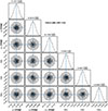 |
Fig. B.1. Example of the posterior distribution from the Bayesian refinement analysis for the OGLE-LMC-CEP-1124 star showing the parameter co variances and the statistical uncertainties on the obtained parameters. |
Appendix C: Best-fitting model parameters with set D equivalent TC parameters
The following table presents the best-fitting model parameters for the plot shown in Fig. 2.
Best-fit model parameters: mass, luminosity, effective temperature, MESA-RSP TC parameters, etc.
Appendix D: Best-fit model parameters with set D equivalent TC parameters
Table D.1 presents the best-fitting model parameters obtained after the inclusion of the TC parameters αp, αt, and/or γr in the convection theory. A comparison plot between set A and set D equivalent parameters and corelation between periods and surface velocity amplitud are shown in Fig. D.1 and Fig. D.2, respectively.
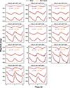 |
Fig. D.1. Best-fit models with the set D equivalent convection parameters overplotted with those with set A parameters. |
Best-fit model parameters with equivalent set D TC parameters, including mass, luminosity, effective temperature, and the MESA-RSP TC parameters.
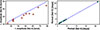 |
Fig. D.2. Comparison of surface velocity amplitude (on the left) and period (on the right) between set A and set D equiv models. While the periods and light curve amplitudes show good agreement, some differences are noted in the surface velocity amplitudes. |
All Tables
Fiducial turbulent convective parameter sets as reported in Paxton et al. (2019).
Best-fit model parameters: mass, luminosity, effective temperature, MESA-RSP TC parameters, etc.
Best-fit model parameters with equivalent set D TC parameters, including mass, luminosity, effective temperature, and the MESA-RSP TC parameters.
All Figures
|
Fig. 1. Location of the Cepheids selected in this work on the HRD. The IS edges are taken from Deka et al. (2024). |
| In the text | |
|
Fig. 2. Observed light curves (data points) for OGLE-LMC-CEP-1124 star is shown along with the best-fitting model predictions overlaid on all the computed models for this star. The χ2 values of the models range from 1.3 (best-fit model) to 49.4 (worst-fit model). |
| In the text | |
|
Fig. 3. Observed light curves (data points) for the selected Cepheids with the best-fitting model predictions overplotted as continuous lines. |
| In the text | |
|
Fig. 4. Observed light curves (data points) for five selected Cepheids with the best-fitting model predictions from MESA-RSP and Stellinwerf code overplotted as continuous lines. |
| In the text | |
|
Fig. 5. Comparison between the reddened distance moduli (in the V, I, and Ks bands) and stellar radii derived in this work with those reported by R19. Each panel shows the respective comparison, including the error bars on the distance moduli, showing the consistency and deviations across photometric bands and radius estimates. |
| In the text | |
|
Fig. 6. Correlations between the stellar parameters and the TC parameters ( |
| In the text | |
|
Fig. 7. ML, PR, and PMR relations derived from our best-fit model set. Two distinct relations for FU and FO cepheids are clearly distinct in each case. |
| In the text | |
|
Fig. 8. PL and PW relations in the V, I, and Ks-bands derived from out best-fit model set. The relations are in very good agreement with that in R19. |
| In the text | |
|
Fig. B.1. Example of the posterior distribution from the Bayesian refinement analysis for the OGLE-LMC-CEP-1124 star showing the parameter co variances and the statistical uncertainties on the obtained parameters. |
| In the text | |
|
Fig. D.1. Best-fit models with the set D equivalent convection parameters overplotted with those with set A parameters. |
| In the text | |
|
Fig. D.2. Comparison of surface velocity amplitude (on the left) and period (on the right) between set A and set D equiv models. While the periods and light curve amplitudes show good agreement, some differences are noted in the surface velocity amplitudes. |
| In the text | |
Current usage metrics show cumulative count of Article Views (full-text article views including HTML views, PDF and ePub downloads, according to the available data) and Abstracts Views on Vision4Press platform.
Data correspond to usage on the plateform after 2015. The current usage metrics is available 48-96 hours after online publication and is updated daily on week days.
Initial download of the metrics may take a while.