© The Authors 2025

1. Introduction

The main properties of hot and dilute plasmas in space appear to be self-regulated through multi-scale mechanisms, and the desire to understand these mechanisms has stimulated observational exploration (Kasper et al. 2002; Salem et al. 2003; Štverák et al. 2008; Bale et al. 2009; Maruca et al. 2012; Huang et al. 2020; Martinović et al. 2021; Salem et al. 2023; Short et al. 2024) as well as theoretical and numerical modeling (Marsch et al. 2006; Matteini et al. 2007; Ofman et al. 2014; Innocenti et al. 2019; Micera et al. 2020; Yoon et al. 2024a,b; Echeverría-Veas et al. 2024; Shaaban et al. 2025). Worth mentioning are the macroscopic models that seek to explain the influence of non-adiabatic expansion of the solar wind (Marsch et al. 2006; Matteini et al. 2007; Innocenti et al. 2019; Seough et al. 2023; Echeverría-Veas et al. 2024), but also the kinetic or small-scale approaches aimed at providing explanations for kinetic anisotropies and departures from quasi-steady states of energy equipartition (Ofman et al. 2014; Maneva et al. 2015; Yoon et al. 2024a; Ofman et al. 2025).

The role of kinetic instabilities, self-generated by the anisotropies of velocity distributions measured in situ, has been intensively investigated both for low-energy quasi-thermal populations (Gary 1993; Yoon 2017; Klein et al. 2019) and for suprathermal components (Shaaban et al. 2021; López et al. 2021), while relaxation due to particle-particle collisions has received more attention only recently (Vafin et al. 2019; Yoon et al. 2024a,b). The constraining effects of the kinetic instabilities are fast enough to explain the observed quasi-steady states, which are generally below the anisotropy thresholds of the instabilities (Kasper et al. 2002; Štverák et al. 2008; Shaaban et al. 2025). Binary collisions, on the other hand, require a different approach, given that the mean free paths (λ_mfp) also increase not only with particle velocity (λ_mfp ∝ v⁴) (Maksimovic et al. 1997), but also with heliospheric distance, becoming, for instance, λ_mfp ∼ 1 au at 1 au (Pierrard et al. 2011). Despite the weakly collisional or even collisionless nature of the solar wind plasma at 1 au, major populations, such as low-energy cores, retain Maxwellian-shaped distributions typical of collision-dominated populations, and quasi-stationary states gather around conditions of isotropy and energy equipartition, still with large collisional ages acquired in the outer corona (Salem et al. 2003; Kasper et al. 2003; Štverák et al. 2008).

It is thus expected that coronal low-beta (β < 1) plasma parcels (where β is the ratio of particle kinetic and magnetic field energy densities) will retain their collision imprint, even during distant heliospheric travel. Relevant are the quasi-stationary states revealed by in situ measurements, which group into the already known rhombic shapes in (β_∥, T_⊥/T_∥) phase space, where T_⊥, ∥ are temperatures in the perpendicular or parallel directions with respect to the ambient magnetic field (Matteini et al. 2007; Štverák et al. 2008; Bale et al. 2009; Maruca et al. 2012; Huang et al. 2020). Here, β_∥ = 8πnT_∥/B₀² is the ratio of (parallel) thermal versus magnetic field energy densities. Thus, self-excited instabilities can be invoked to constrain the limits of these states toward high β > 1 values – but not the other limits toward low β < 1 values. A series of recent studies have shown that – in the case of electrons and protons, binary collisions can complete this picture, providing very plausible explanations for low-beta limits as well (Vafin et al. 2019; Yoon et al. 2024a,b).

In this work, we focus on the relaxation of the temperature anisotropy of major ions, namely protons and alpha particles (He⁺⁺), by modeling the quasi-linear regulation of their anisotropies, both through collision processes and instability excitation. Observational data have already been compared with the predictions of linear theory for the instabilities generated by the temperature anisotropies of protons (Matteini et al. 2007; Bale et al. 2009) and alpha particles (Maruca et al. 2012; Martinović et al. 2025). In our quasi-linear models, we ignore the relative drifts between the two ion species. The relative density of alpha particles to the protons measured in the solar wind near 1 au shows that the average value can be quite low, less than a couple of percent (Alterman et al. 2018; Alterman & Kasper 2019). Similarly, the relative drift speed between the two species when normalized to the local Alfvén speed have also been observed to be quite low, again less than a couple of percent.

Fig. 1. [Left] Probability distribution function for nα/n versus nα/n, showing that the most probable value of nα/n is ∼𝒪(10−2). Those alpha particles satisfying the condition β∥α < 10−2, which turns out to be susceptible to collisional relaxation, are treated separately, and their partial probability distribution function is plotted with blue dots. The opposite condition β∥α > 10−2 turns out to define the solar wind condition susceptible to instability relaxation, and these alpha particles are treated separately. Their partial probability distribution function is plotted with red dots. [Right] Probability distribution function for |Vp − Vα|/VA versus the normalized proton-to-alpha relative drift speed, |Vp − Vα|/VA, showing that the most probable value of |Vp − Vα|/VA is also ∼𝒪(10−2).

In Figure 1 we plot the probability distribution functions for a density ratio, n_α/n, and for a relative proton-alpha drift speed, |V_p − V_α|/V_A. The dataset used for Figure 1 is taken from the WIND spacecraft SWE Faraday Cup observations (Ogilvie et al. 1995). A nonlinear least-squares fitting algorithm was applied to determine the proton and alpha particle velocities, densities, and the magnetic field intensity (Maruca & Kasper 2013). As can be seen from Figure 1, the most probable values of n_α/n and |V_p − V_α|/V_A are ∼𝒪(10⁻²). We further separated the dataset for n_α/n into two subcategories by placing a condition on the parallel alpha particle beta, β_∥α. Specifically, we plot the dataset satisfying the inequality β_∥α < 10⁻² with blue dots and the complementary dataset satisfying the opposite inequality β_∥α > 10⁻² with red dots. The condition β_∥α = 10⁻² roughly defines the demarcation for alpha particles controlled by collisions versus instabilities. Such a delineation between the collision-dominated versus collision-free solar wind has been considered in the literature – e.g., see Kasper et al. (2017) – and for our purpose, we find that β_∥α is a useful quantity in this regard.

Our paper is structured as follows: In Section 2 we formulate the theory of collisional temperature anisotropy relaxation for protons and alpha particles. We carried out the ensemble simulation based on the collisional relaxation theory, and we make a comparison to the observation. In Section 3 we formulate the quasi-linear theory of temperature anisotropy relaxation for protons and alpha particles in the absence of binary collisions. In this case, the relaxation mechanism is based on the temperature anisotropy-driven collective instabilities and subsequent saturation. For the sake of simplicity, we carried out the quasi-linear ensemble calculation with the assumption of parallel propagation of waves and instabilities. We compare the outcome of the quasi-linear ensemble calculation against the observation made in the near-Earth space environment. We summarize the findings in Section 4, and some additional details regarding technical issues are presented in Appendix A.

2. Collisional temperature relaxation for the proton-alpha particle system

The equations that describe the relaxation of anisotropic temperatures by collisional processes among multiple charged particle species are discussed in Yoon et al. (2024b). The starting point of the present discussion is equation (A7) in Appendix A of Yoon et al. (2024b), which we reproduce below:

$$\begin{array}{cc}\hfill \frac{\mathrm{d}{T}_{\perp a}}{\mathrm{d}t}& ={\displaystyle \sum _b}\frac{8{\left(2\pi \right)}^{\frac{1}{2}}{n}_b{e}_a^2{e}_b^{2}ln\mathrm{\Lambda }}{15m_a{(T_{\Vert a}/m_a+T_{\Vert b}/m_b)}^{\frac{3}{2}}}(\frac{T_{\Vert a}}{m_a}-\frac{T_{\perp a}}{m_a}+\frac{4T_{\perp b}}{m_b}-\frac{5T_{\perp a}}{m_b}+\frac{T_{\Vert b}}{m_b}),\hfill \\ \hfill \frac{\mathrm{d}{T}_{\Vert a}}{\mathrm{d}t}& ={\displaystyle \sum _b}\frac{16{\left(2\pi \right)}^{\frac{1}{2}}{n}_b{e}_a^2{e}_b^{2}ln\mathrm{\Lambda }}{15m_a{(T_{\Vert a}/m_a+T_{\Vert b}/m_b)}^{\frac{3}{2}}}(\frac{T_{\perp a}}{m_a}-\frac{T_{\Vert a}}{m_a}+\frac{T_{\perp b}}{m_b}+\frac{3}{2}\frac{T_{\Vert b}}{m_b}-\frac{5}{2}\frac{T_{\Vert a}}{m_b}).\hfill \end{array}$$(1)

The species labels a = e, p, α and b = e, p, α stand for electrons (e), protons (p), and alpha particles (α); m_a, e_a, and n_b respectively denote the mass, unit charge, and the number density for each charged particle species; T_⊥a and T_∥b are perpendicular and parallel temperatures for each particle species; and lnΛ is the Coulomb logarithm, where Λ = 4πn_eλ_De³. Here, λ_De = [T_e/(4πn_ee²)]^1/2 is the Debye length. For the proton-alpha particle system with background electrons, we make use of e_α = 2e and m_α = 4m_p as well as the charge neutrality condition, n_p + 2n_α − n_e = 0 (or equivalently, n = n_e = n_p + 2n_α). Upon explicitly writing down the temperature evolution equations for each charged particle species, namely, electrons, protons, and alpha particles, we simplified the resulting expressions by neglecting terms proportional to the electron-to-proton mass ratio and its square root, that is, terms of the order (m_e/m_p)^1/2, (m_e/m_p) or lower. After some tedious but otherwise straightforward algebraic manipulations, we find that the resultant equations are given by

$$\begin{array}{cc}\hfill \frac{\mathrm{d}{T}_{\perp e}}{\mathrm{d}t}& ={\nu }_{\mathit{ee}}(1+\frac{2^{\frac{1}{2}}(n_p+4n_{\alpha })}{n})(T_{\Vert e}-T_{\perp e}),\hfill \\ \hfill \frac{\mathrm{d}{T}_{\Vert e}}{\mathrm{d}t}& =2{\nu }_{\mathit{ee}}(1+\frac{2^{\frac{1}{2}}(n_p+4n_{\alpha })}{n})(T_{\perp e}-T_{\Vert e}),\hfill \\ \hfill \frac{\mathrm{d}{T}_{\perp p}}{\mathrm{d}t}& =({\nu }_{\mathit{pp}}\frac{n_p}{n}+{\nu }_{p\alpha }\frac{4n_{\alpha }}{n})(T_{\Vert p}-T_{\perp p})+{\nu }_{p\alpha }\frac{n_{\alpha }}{n}(T_{\perp \alpha }-T_{\perp p}),\hfill \\ \hfill \frac{\mathrm{d}{T}_{\Vert p}}{\mathrm{d}t}& =2({\nu }_{\mathit{pp}}\frac{n_p}{n}+{\nu }_{p\alpha }\frac{4n_{\alpha }}{n})(T_{\perp p}-T_{\Vert p})+{\nu }_{p\alpha }\frac{n_{\alpha }}{n}(T_{\perp \alpha }-T_{\perp p}),\hfill \\ \hfill \frac{\mathrm{d}{T}_{\perp \alpha }}{\mathrm{d}t}& =({\nu }_{\alpha \alpha }\frac{n_{\alpha }}{n}+{\nu }_{p\alpha }\frac{n_p}{4n})(T_{\Vert \alpha }-T_{\perp \alpha })+{\nu }_{p\alpha }\frac{n_p}{n}(T_{\perp p}-T_{\perp \alpha }),\hfill \\ \hfill \frac{\mathrm{d}{T}_{\Vert \alpha }}{\mathrm{d}t}& =2({\nu }_{\alpha \alpha }\frac{n_{\alpha }}{n}+{\nu }_{p\alpha }\frac{n_p}{4n})(T_{\perp \alpha }-T_{\Vert \alpha })+{\nu }_{p\alpha }\frac{n_p}{n}(T_{\perp p}-T_{\perp \alpha }),\hfill \end{array}$$(2)

where various collisional frequencies are defined by

$$\begin{array}{cc}\hfill {\nu }_{\mathit{ee}}& ={\left(\frac{\pi }{m_e}\right)}^{\frac{1}{2}}\frac{8n{e}^{4}ln\mathrm{\Lambda }}{15T_{\Vert e}^{\frac{3}{2}}},{\nu }_{\mathit{pp}}={\left(\frac{\pi }{m_p}\right)}^{\frac{1}{2}}\frac{8n{e}^{4}ln\mathrm{\Lambda }}{15T_{\Vert p}^{\frac{3}{2}}},{\nu }_{\alpha \alpha }={\left(\frac{\pi }{m_p}\right)}^{\frac{1}{2}}\frac{64n{e}^{4}ln\mathrm{\Lambda }}{15T_{\Vert \alpha }^{\frac{3}{2}}},{\nu }_{p\alpha }={\left(\frac{2\pi }{m_p}\right)}^{\frac{1}{2}}\frac{64n{e}^{4}ln\mathrm{\Lambda }}{5{(4T_{\Vert p}+T_{\Vert \alpha })}^{\frac{3}{2}}}.\hfill \end{array}$$(3)

It can easily be shown that Equation (2) satisfies the energy conservation relationships:

$$\begin{array}{cc}& 2T_{\perp e}+T_{\Vert e}=\mathrm{const},n_p(2T_{\perp p}+T_{\Vert p})+n_{\alpha }(2T_{\perp a}+T_{\Vert \alpha })=\mathrm{const}.\hfill \end{array}$$(4)

Note that the electron temperature relaxation proceeds at a much faster rate than the ion temperature relaxation. In particular, the timescale of electron dynamics is faster by a factor of (m_p/m_e)^1/2. This is because the very light electrons and heavier ions (protons and alpha particles) move at disparate timescales. As a consequence, the electrons may be treated as essentially isotropic and assume that they simply follow the ions in an adiabatic sense. We thus ignored the electron temperature equations and only considered the ion dynamics. Of course, electron dynamics can be incorporated in the present discussion, but we treat the combined proton and alpha particle dynamics separately from that of the electrons for the sake of simplicity.

Henceforth, we adopt the same normalization scheme first introduced in our previous paper (Yoon et al. 2024a), which was also adopted in a subsequent paper (Yoon et al. 2024b), where we normalize the time variable with respect to the proton gyro-frequency, Ω_p = eB/m_pc. Here, c is the speed of light and B is the ambient magnetic field intensity. The dimensionless temperatures are expressed via plasma betas, that is, the ratio of thermal to magnetic field energy densities. The ratio of alpha particle density to the total density (which is equal to the electron density) is defined by

$$\begin{array}{c}\hfill \delta =n_{\alpha }/n.\end{array}$$(5)

The various collision frequencies are normalized by the proton gyro-frequency. With this normalization convention, all the dimensionless physical quantities that pertain to the present paper can be directly compared with the same quantities and expressions found in our previous two papers (Yoon et al. 2024a,b),

$$\begin{array}{cc}& \tau ={\mathrm{\Omega }}_{p}t,{\beta }_{\perp ,\Vert a}=\frac{8\pi n_a{T}_{\perp ,\Vert a}}{B^2},g=\frac{\sqrt{2}}{{\pi }^{3/2}}\frac{1}{n{(c/{\omega }_{\mathit{pp}})}^3}\frac{c^4}{v_A^4}=7.76\times {10}^{-27}\frac{n_{[\mathrm{pcc}]}^{5/2}}{B_{[\mathrm{Gauss}]}^4},ln\mathrm{\Lambda }=ln\frac{5.16\times {10}^9{T}_{[\mathrm{eV}]}^{3/2}}{n_{[\mathrm{pcc}]}^{1/2}},\hfill \end{array}$$(6)

where T_[eV] represents a reference electron temperature (given in eV), n_[pcc] is the background plasma density (given in number of particles per cubic centimeter or pcc), and B_[Gauss] is the magnetic field intensity (given in gauss), respectively; ω_pp = (4πne²/m_p)^1/2 and v_A = B/(4πnm_p)^1/2 represent the proton plasma oscillation frequency and the Alfvén speed, respectively. The normalized equations are

$$\begin{array}{cc}\hfill \frac{\mathrm{d}{\beta }_{\perp p}}{\mathrm{d}\tau }& ={\mu }_{\mathit{pp}}({\beta }_{\Vert p}-{\beta }_{\perp p})+{\mu }_{p\alpha }[(1-2\delta ){\beta }_{\perp \alpha }-\delta {\beta }_{\perp p}],\hfill \\ \hfill \frac{\mathrm{d}{\beta }_{\Vert p}}{\mathrm{d}\tau }& =-2{\mu }_{\mathit{pp}}({\beta }_{\Vert p}-{\beta }_{\perp p})+{\mu }_{p\alpha }[(1-2\delta ){\beta }_{\perp \alpha }-\delta {\beta }_{\perp p}],\hfill \\ \hfill \frac{\mathrm{d}{\beta }_{\perp \alpha }}{\mathrm{d}\tau }& ={\mu }_{\alpha \alpha }({\beta }_{\Vert \alpha }-{\beta }_{\perp \alpha })-{\mu }_{p\alpha }[(1-2\delta ){\beta }_{\perp \alpha }-\delta {\beta }_{\perp p}],\hfill \\ \hfill \frac{\mathrm{d}{\beta }_{\Vert \alpha }}{\mathrm{d}\tau }& =-2{\mu }_{\alpha \alpha }({\beta }_{\Vert \alpha }-{\beta }_{\perp \alpha })-{\mu }_{p\alpha }[(1-2\delta ){\beta }_{\perp \alpha }-\delta {\beta }_{\perp p}],\hfill \\ \hfill {\mu }_{\mathit{pp}}& =g\prime (\frac{{(1-2\delta )}^{\frac{5}{2}}}{{\beta }_{\Vert p}^{\frac{3}{2}}}+\frac{32\sqrt{2}{\delta }^{\frac{5}{2}}{(1-2\delta )}^{\frac{3}{2}}}{{[4\delta {\beta }_{\Vert p}+(1-2\delta ){\beta }_{\Vert \alpha }]}^{\frac{3}{2}}}),{\mu }_{\alpha \alpha }=2g\prime (\frac{4{\delta }^{\frac{5}{2}}}{{\beta }_{\Vert \alpha }^{\frac{3}{2}}}+\frac{\sqrt{2}{\delta }^{\frac{3}{2}}{(1-2\delta )}^{\frac{5}{2}}}{{[4\delta {\beta }_{\Vert p}+(1-2\delta ){\beta }_{\Vert \alpha }]}^{\frac{3}{2}}}),\hfill \\ \hfill {\mu }_{p\alpha }& =g\prime \frac{40\sqrt{2}{\delta }^{\frac{3}{2}}{(1-2\delta )}^{\frac{3}{2}}}{{[4\delta {\beta }_{\Vert p}+(1-2\delta ){\beta }_{\Vert \alpha }]}^{\frac{3}{2}}},g\prime =\frac{gln\mathrm{\Lambda }}{15}.\hfill \end{array}$$(7)

As with our previous two papers, we took the typical 1 au value for the plasma density, n ∼ 8 cm⁻³; the magnetic field intensity, B ∼ 5nT = 5 × 10⁻⁵ Gauss; and the reference electron temperature, T_e ∼ 140 000 K ∼ 12 eV (Wilson et al. 2018; Klein & Vech 2019). Taking the typical solar wind speed of ∼300–600 km/sec, we arrive at the estimation of the transit time between the solar source to the distance of 1.496 × 10⁸ km (that is, 1 au) to be ∼2.5 × 10⁵–5 × 10⁵ sec. That is, we choose the same parameters as in Yoon et al. (2024a,b),

$$\begin{array}{c}\hfill g\prime =\frac{gln\mathrm{\Lambda }}{15}\simeq {10}^{-7},{\tau }_{\max }\sim {10}^4\mathrm{to}5\times {10}^4.\end{array}$$(8)

As with our previous study on the core and halo electrons dynamics (Yoon et al. 2024b), we consider a hypothetical ensemble of “initial” solar wind states. We considered separate initial ensembles of protons and alphas. These initial ensemble states were presumed to be associated with regions close to the coronal source and propagate to the near-Earth vicinity. As we stated in our previous papers, our purpose is not to model the realistic solar wind conditions close to the solar source (Huang et al. 2020; Mostafavi et al. 2024). Rather, our purpose is to cover a wide range of phase space uniformly with an appropriate choice of hypothetical ensembles of protons and alpha particles at the initial time. We emphasize that there are many possible combinations of initial states, as also stated previously in our paper (Yoon et al. 2024b), but in Figure 2, we display one specific combination where the respective proton and alpha particle ensemble points are arranged in a manner that has a prescribed repeating pattern for both species. Specifically, for case 1, we set both the proton and alpha particle initial states as occupying the upper-left corner points in their respective beta-anisotropy phase spaces, namely, β_∥α = 10^−4.8, T_⊥α/T_∥α = 10^1.2 – and β_∥p = 10^−2.75, T_⊥p/T_∥p = 10^0.8. In case 2, the proton and alpha particle states are chosen as the points immediately below those of case 1, that is, all the parameters are the same except that the temperature ratio is slightly lower for both the protons and alpha particles: T_⊥α/T_∥α = 10^0.9, T_⊥p/T_∥p = 10^0.6. Then for case 3, we chose T_⊥α/T_∥α = 10^0.6, T_⊥p/T_∥p = 10^0.4. We continued in this manner until we reach case 9, for which the temperature ratios are T_⊥α/T_∥α = 10^−1.2 and T_⊥p/T_∥p = 10^−0.8, respectively. We then repeated the pattern with slightly higher values of parallel betas, namely, β_∥α = 10^−4.45 and β_∥p = 10^−2.5 (cases 10 to 18). For the next set of nine cases, the corresponding beta values are β_∥α = 10^−4.1 and β_∥p = 10^−2.25, so on and so forth. Figure 2 shows this particular arrangement with each case indicated by the corresponding number. As mentioned in our previous paper (Yoon et al. 2024b), one could reshuffle the initial ensemble positions in any arbitrary combination, which could improve the present type of analysis, but we prefer to consider this particular arrangement of initial conditions for the sake of simplicity.

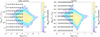Fig. 2. [Left] Initial ensemble positions of alpha particles plotted against a background showing the alpha particle data distribution. [Right] Same but for the protons – and plotted against a backdrop showing the proton 2D distribution. The numerical designations signify the case numbers: 1 to 81.

In the background of the panels in Figure 2, we have plotted the color map of the occurrence distributions for the solar wind alpha particles and protons. The left panel shows the initial alpha particle ensemble points, and the right panel showing the same but for the protons. The color-shaded alpha and proton data distributions use measurements from WIND spacecraft SWE Faraday Cup observations (Ogilvie et al. 1995), to which we applied a nonlinear least squares fitting algorithm to determine solar wind proton and alpha particle velocity moments, namely density, bulk speed, temperature, and temperature anisotropy (Maruca & Kasper 2013).

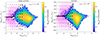Fig. 3. [Left] Initial ensemble of alpha particle data points plotted with open circles. The dynamic paths in (β∥α, T⊥α/T∥α) space are indicated with magenta curves, and the final states at τmax = Ωptmax = 2 × 104 are marked with black dots. In the background is the alpha particle data distribution. [Right] Same but for the protons. (An associated movie is available online)

We solved the dynamical Equation (7) under input parameters corresponding to the estimate given in equation (8), namely, g′ = 10⁻⁷ and τ_max = 10⁴ to 5 × 10⁴. These normalized input parameters are identical to those adopted in our earlier study on the protons and core-halo electron system (Yoon et al. 2024a,b). As shown in Figure 1 and confirmed by Figure 2, the alpha particles (He⁺⁺) satisfying the approximate inequality condition β_∥α < 10⁻² can be considered as susceptible to collisions. For such a case, Figure 1 shows that the characteristic value of δ is roughly ∼𝒪(10⁻²). We thus made the choice of δ = 0.01. In the left panel of Figure 3, the initial ensemble of alpha particle data points is plotted with open circles (the left panel is identical to that of Figure 2). The ensemble of points are plotted in the background of the alpha particle data distribution (2D histogram), as in Figure 2. The dynamic paths in (β_∥α, T_⊥α/T_∥α) space are indicated with magenta curves. The alpha particles reach the final states, which we chose to be τ_max = Ω_pt_max = 2 × 10⁴, as they relax via the collisional processes. In the figure, the final states are marked with black dots. The concomitant solutions for the protons are plotted in Figure 3 in the right panel. The format is the same as with the alpha particles. We note that the maximum travel time chosen in our earlier papers (Yoon et al. 2024a,b) corresponds to τ_max = 5 × 10⁴, whereas in this paper we terminated the collisional relaxation calculation at τ_max = 2 × 10⁴. However, from the associated movie available online, the relaxation process reaches a virtual steady state by the time the computation proceeds to τ_max = 2 × 10⁴ such that additional computation beyond this point is not terribly meaningful. We present the entire course of alpha particle and proton ensemble evolution in the accompanying video, which shows that the early-time evolution is quite rapid, but the evolution rapidly slows down and reaches a virtual steady state quite early on, around τ = 10⁴. The time step in the video corresponds to Δτ = 200, and the animation runs until τ = 2 × 10⁴. The additional evolution between τ = 10⁴ and τ_max = 2 × 10⁴ is incremental.

Based on the accompanying movie as well as both panels in Figure 3, it can be seen that the “initial” ensemble points that are at a sufficient distance outside the boundary of the data distributions – for both alpha particles and protons – move swiftly toward and settle around the outer perimeters on the low-beta sides of the respective data distributions. In contrast, the ensemble points already located within the respective data distributions either barely move or move only slightly. This finding is consistent with our earlier work on the protons (Yoon et al. 2024a) and electrons (Yoon et al. 2024b) in that the collisional relaxation process is indeed a baseline explanation for the boundary of the charged particle and sub-particle species distributions on the low-beta side, as observed in the solar wind near 1 au.

3. Regulation of proton-alpha particle temperature anisotropies by collective instability excitation

The quasi-linear velocity moment equation for temperature relaxation under the assumption of bi-Maxwellian proton and alpha particle velocity distribution functions was derived by Yoon et al. (2015). The derivation was done under the assumption that transverse electromagnetic perturbations propagate along the direction of the ambient magnetic field, thus excluding the impact of obliquely propagating instabilities. This is an obvious approximation, but we adopted this formalism for the sake of simplicity. The set of equations describing the quasi-linear instability process is given by

$$\begin{array}{cc}\hfill \frac{\mathrm{d}{T}_{\perp p}}{\mathrm{d}t}& =-\frac{e^2}{2m_p{c}^2}{\displaystyle \int \frac{\mathrm{d}k}{k^2}}{\displaystyle \sum _{+,-}}\delta B_{\pm }^2(k)\{(2A_p+1){\gamma }_k+\mathrm{Im}\left[(2i{\gamma }_k\pm {\mathrm{\Omega }}_p){\eta }_{\pm }^{p}Z\left({\zeta }_{\pm }^p\right)\right]\},\hfill \\ \hfill \frac{\mathrm{d}{T}_{\Vert p}}{\mathrm{d}t}& =\frac{e^2}{m_p{c}^2}{\displaystyle \int \frac{\mathrm{d}k}{k^2}\sum _{+,-}}\delta B_{\pm }^2(k)\{(A_p+1){\gamma }_k+\mathrm{Im}\left[(\omega \pm {\mathrm{\Omega }}_p){\eta }_{\pm }^{p}Z\left({\zeta }_{\pm }^p\right)\right]\},\hfill \\ \hfill \frac{\mathrm{d}{T}_{\perp \alpha }}{\mathrm{d}t}& =-\frac{e^2}{2m_p{c}^2}{\displaystyle \int \frac{\mathrm{d}k}{k^2}\sum _{+,-}}\delta B_{\pm }^2(k)\{(2A_{\alpha }+1){\gamma }_k+\mathrm{Im}\left[(2i{\gamma }_k\pm \frac{1}{2}{\mathrm{\Omega }}_p){\eta }_{\pm }^{\alpha }Z({\zeta }_{\pm }^{\alpha })\right]\},\hfill \\ \hfill \frac{\mathrm{d}{T}_{\Vert \alpha }}{\mathrm{d}t}& =\frac{e^2}{m_p{c}^2}{\displaystyle \int \frac{\mathrm{d}k}{k^2}\sum _{+,-}}\delta B_{\pm }^2(k)\{(A_{\alpha }+1){\gamma }_k+\mathrm{Im}\left[(\omega \pm \frac{1}{2}{\mathrm{\Omega }}_p){\eta }_{\pm }^{\alpha }Z({\zeta }_{\pm }^{\alpha })\right]\},\hfill \\ \hfill A_p& =\frac{T_{\perp p}}{T_{\Vert p}}-1,A_{\alpha }=\frac{T_{\perp \alpha }}{T_{\Vert \alpha }}-1,\hfill \\ \hfill {\eta }_{\pm }^p& =\frac{(A_p+1)\omega \pm A_p{\mathrm{\Omega }}_p}{k{\alpha }_{\Vert p}},{\eta }_{\pm }^{\alpha }=\frac{(A_{\alpha }+1)\omega \pm A_{\alpha }{\mathrm{\Omega }}_p/2}{k{\alpha }_{\Vert \alpha }},{\zeta }_{\pm }^p=\frac{\omega \pm {\mathrm{\Omega }}_p}{k{\alpha }_{\Vert p}},{\zeta }_{\pm }^{\alpha }=\frac{\omega \pm {\mathrm{\Omega }}_p/2}{k{\alpha }_{\Vert \alpha }},\hfill \end{array}$$(9)

where we made use of e_α²/m_α = e²/m_p, and where ω = ω_k + iγ_k denotes the complex conjugate solutions of the dispersion relation

$$\begin{array}{c}\hfill 0=\frac{c^2{k}^2}{{\omega }_{\mathit{pp}}^2}\mp \frac{\omega }{{\mathrm{\Omega }}_p}-{\displaystyle \sum _{a=p,\alpha }}\frac{n_a}{n}[A_a+{\eta }_a^{\pm }Z\left({\zeta }_a^{\pm }\right)].\end{array}$$(10)

In the above equation, the plus and minus signs respectively signify the right-hand circularly polarized firehose (FH) mode and the left-hand circularly polarized electromagnetic ion-cyclotron (EMIC) mode. The spectral magnetic field wave energy density corresponding to the left or right mode, δB_±²(k), satisfies the wave kinetic equation,

$$\begin{array}{c}\hfill \frac{\partial }{\partial t}\delta B_{\pm }^2(k)=2{\gamma }_k\delta B_{\pm }^2(k).\end{array}$$(11)

It is interesting to note that the quasi-linear velocity moment Equation (9) satisfies a separate energy conservation relationship given by

$$\begin{array}{c}\hfill n_p(2T_{\perp p}+T_{\Vert p})+n_{\alpha }(2T_{\perp \alpha }+T_{\Vert \alpha })+{\mathcal{E}}_B=\mathrm{const},\end{array}$$(12)

which is distinct from its collisional counterpart, Equation (4), for the presence of total wave magnetic field energy density,

$$\begin{array}{c}\hfill {\mathcal{E}}_B\equiv {\displaystyle \sum _{+,-}}{\displaystyle \int \mathrm{d}}k\frac{\delta B_{\pm }^2(k)}{8\pi },\end{array}$$(13)

on the left-hand side.

We can write the set of equations in terms of the same dimensionless quantities, which we have already introduced, namely, τ = Ω_pt, β_⊥, ∥a = 8πn_aT_⊥, ∥a/B₀², δ = n_α/n, and A_a = T_⊥a/T_∥a − 1 = β_⊥a/β_∥a − 1, as well as in terms of additional normalized variables,

$$\begin{array}{cc}& z_r=\frac{{\omega }_k}{{\mathrm{\Omega }}_p},z_i=\frac{{\gamma }_k}{{\mathrm{\Omega }}_p},q=\frac{\mathit{ck}}{{\omega }_{\mathit{pp}}},W_{\pm }(q)\mathrm{d}q=\frac{\delta B_{\pm }^2(k)}{B_0^2}\mathrm{d}k.\hfill \end{array}$$(14)

The result is

$$\begin{array}{cc}\hfill \frac{\mathrm{d}{\beta }_{\perp p}}{\mathrm{d}\tau }& =-(1-2\delta ){\displaystyle \int \frac{\mathrm{d}q}{q^2}\sum _{+,-}}{W}_{\pm }(q)\{(2A_p+1)z_i+\mathrm{Im}\left[(2i{z}_i\pm 1){\eta }_{\pm }^{p}Z\left({\zeta }_{\pm }^p\right)\right]\},\hfill \\ \hfill \frac{\mathrm{d}{\beta }_{\Vert p}}{\mathrm{d}\tau }& =2(1-2\delta ){\displaystyle \int \frac{\mathrm{d}q}{q^2}\sum _{+,-}}{W}_{\pm }(q)\{(A_p+1)z_i+\mathrm{Im}\left[(z\pm 1){\eta }_{\pm }^{p}Z\left({\zeta }_{\pm }^p\right)\right]\},\hfill \\ \hfill \frac{\mathrm{d}{\beta }_{\perp \alpha }}{\mathrm{d}\tau }& =-\delta {\displaystyle \int \frac{\mathrm{d}q}{q^2}\sum _{+,-}}{W}_{\pm }(q)\{(2A_{\alpha }+1)z_i+\mathrm{Im}\left[(2i{z}_i\pm \frac{1}{2}){\eta }_{\pm }^{\alpha }Z\left({\zeta }_{\pm }^{\alpha }\right)\right]\},\hfill \\ \hfill \frac{\mathrm{d}{\beta }_{\Vert \alpha }}{\mathrm{d}\tau }& =2\delta {\displaystyle \int \frac{\mathrm{d}q}{q^2}\sum _{+,-}}{W}_{\pm }(q)\{(A_{\alpha }+1)z_i+\mathrm{Im}\left[(z\pm \frac{1}{2}){\eta }_{\pm }^{\alpha }Z\left({\zeta }_{\pm }^{\alpha }\right)\right]\},\hfill \\ \hfill {\eta }_{\pm }^p& =\frac{(A_p+1)z\pm A_p}{q{[{\beta }_{\Vert p}/(1-2\delta )]}^{\frac{1}{2}}},{\eta }_{\pm }^{\alpha }=\frac{(A_{\alpha }+1)z\pm \frac{1}{2}{A}_{\alpha }}{q{[{\beta }_{\Vert \alpha }/\left(4\delta \right)]}^{\frac{1}{2}}},{\zeta }_{\pm }^p=\frac{z\pm 1}{q{[{\beta }_{\Vert p}/(1-2\delta )]}^{\frac{1}{2}}},{\zeta }_{\pm }^{\alpha }=\frac{z\pm \frac{1}{2}}{q{[{\beta }_{\Vert \alpha }/\left(4\delta \right)]}^{\frac{1}{2}}},\hfill \\ \hfill \frac{\partial W_{\pm }(q)}{\partial \tau }& =2z_i{W}_{\pm }(q).\hfill \end{array}$$(15)

As with our earlier discussion regarding the core and halo electron problem, we also found that the numerical complex root solving routine based on the exact instantaneous dispersion relation (10) is quite cumbersome. As with our previous paper (Yoon et al. 2024b), the present situation that involves protons combined with the alpha particles renders the automatic complex root solving scheme at each time step along the quasi-linear computation by numerical means somewhat unreliable. For this reason, we employed a similar approximation as in Yoon et al. (2024b), where the excitation of firehose and EMIC instabilities can be treated by the weak-growth formalism, which assumes that the underlying nature of the wave-particle resonance is that of a resonant type. We found in our earlier work (Yoon et al. 2024b) for the electron firehose instability that the assumption of non-resonant instability is a reasonable first-cut approximation. However, for the present problem of proton-alpha firehose instability, we find that the resonant approximation works quite well, so we implemented the resonant wave-particle interaction approximation uniformly for both the right-hand firehose and the left-hand cyclotron modes. The resulting approximate analysis, the validation of which can be found in Appendix A, led to the following substitutions of the real frequency and growth rate for both the left- and right-hand circularly polarized modes. For the left-hand mode (where the minus sign corresponds to the cyclotron resonance), the normalized real frequency, z_r, is determined by the two positive roots of the cubic equation,

$$\begin{array}{cc}\hfill 0& =(q^2+z_r)(z_r-1)(z_r-\frac{1}{2})+(1-2\delta )z_r(z_r-\frac{1}{2})+\delta z_r(z_r-1),\hfill \end{array}$$(16)

while the normalized real frequency for the right-hand mode (where the plus sign corresponding to the firehose branch) is determined by the negative root of the cubic equation,

$$\begin{array}{cc}\hfill 0& =(q^2+z_r)(z_r+1)(z_r+\frac{1}{2})+(1-2\delta )z_r(z_r+\frac{1}{2})+\delta z_r(z_r+1).\hfill \end{array}$$(17)

The normalized growth rate of the left-hand mode is given by

$$\begin{array}{cc}\hfill z_i& =\frac{{\pi }^{\frac{1}{2}}{(z_r-1)}^2{(z_r-\frac{1}{2})}^2}{R_{-}}[(1-2\delta ){\eta }_{-}^p{e}^{-{\left({\zeta }_{-}^p\right)}^2}+\delta {\eta }_{-}^{\alpha }{e}^{-{\left({\zeta }_{-}^{\alpha }\right)}^2}],\hfill \\ \hfill R_{-}& ={(z_r-1)}^2{(z_r-\frac{1}{2})}^2-(1-2\delta ){(z_r-\frac{1}{2})}^2-\frac{1}{2}\delta {(z_r-1)}^2,\hfill \end{array}$$(18)

where η₋^p, η₋^α, ζ₋^p, and ζ₋^α are defined exactly as in equation (15) (with the minus sign) except that complex normalized frequency, z, is to be replaced by its real part, z_r, which is determined by solving Equation (16). Similarly, the normalized growth rate of the right-hand mode is given by

$$\begin{array}{cc}\hfill z_i& =-\frac{{\pi }^{\frac{1}{2}}{(z_r+1)}^2{(z_r+\frac{1}{2})}^2}{R_{+}}[(1-2\delta ){\eta }_{+}^p{e}^{-{\left({\zeta }_{+}^p\right)}^2}+\delta {\eta }_{+}^{\alpha }{e}^{-{\left({\zeta }_{+}^{\alpha }\right)}^2}],\hfill \\ \hfill R_{+}& ={(z_r+1)}^2{(z_r+\frac{1}{2})}^2-(1-2\delta ){(z_r+\frac{1}{2})}^2-\frac{1}{2}\delta {(z_r+1)}^2.\hfill \end{array}$$(19)

Again, η₊^p, η₊^α, ζ₊^p, and ζ₊^α are defined exactly as in equation (15) (with the plus sign this time) except that the complex normalized frequency, z, is to be replaced by its real part, z_r, which is determined by solving equation (17).

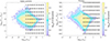Fig. 4. [Left] Initial ensemble positions in the case of collective instability relaxation – for alpha particles: plotted against a background showing the alpha particle data distribution. [Right] Same but for the protons – and plotted against a background showing the proton 2D distribution.

We chose the initial data points for the dual proton and alpha particle populations in the relatively high-beta regime for the purpose of investigating the temperature anisotropy relaxation by collective instability excitation. As with Figure 2, we chose one particular combination of initial ensemble points among many, where the proton and alpha particle (He⁺⁺) data points are arranged in a manner that reflects a systematic repeating pattern. Specifically, for case 1, we placed the alpha particle and proton initial states as occupying the upper-left corner points in the high-beta regime, corresponding to β_∥p = 10^−0.25, T_⊥p/T_∥p = 10^0.8 and β_∥α = 10^−1.7, T_⊥α/T_∥α = 10^1.2. For case 2, it is the same except for the temperature ratio: T_⊥p/T_∥p = 10^0.6, T_⊥α/T_∥α = 10^0.9, so on and so forth, until we reached case 9. We then repeated the pattern with a slightly higher value of parallel betas, namely, β_∥p = 10⁰ and β_∥α = 10^−1.35, and so forth, in a systematic manner until case 81. This pattern is analogous to Figure 2, except that these points occupy the high-beta regime. Figure 4 displays this particular arrangement with each case indicated by the corresponding case number. As with Figure 2, one could reshuffle the relative initial positions of proton and alpha particles in any arbitrary arrays, but we chose this specific initial ensemble arrangement for the sake of convenience. As shown in Figure 1 and indicated by Figure 4, the alpha particles (He⁺⁺) satisfying the condition β_∥α > 10⁻² can be considered as susceptible to instability excitation and relaxation. For this case, for which β_∥α > 10⁻² for all the initial ensemble points, Figure 1 shows that the characteristic value of δ occupies a range somewhat higher than that corresponding to the collisional relaxation. We thus made the choice of δ = 0.05 in the present case of instability relaxation.

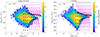Fig. 5. [Left] Initial ensemble of alpha particle data points in the case of relaxation by instability excitation (plotted with open circles). The dynamic paths in (β∥α, T⊥α/T∥α) space are indicated with magenta curves and the final states at τmax = Ωptmax = 50 are marked with black dots. The background shows the alpha particle data distribution. [Right] Same but for the protons. An associated movie showing the entire dynamic paths for the ensemble points that are subject to instability excitation and quasi-linear relaxation is available online.

We solved the dynamical Equation (15) together with the wave kinetic equation. In Figure 5 we have plotted the result of numerical computation. We considered the maximum dimensionless time to correspond to τ_max = Ω_pt_max = 50, which is arbitrary. However, as the associated movie (available online) shows, τ_max = 50 is sufficient to quite accurately capture the essence of the quasi-linear relaxation. In the left panel of Figure 5, which shows the alpha particle dynamics, it can be seen that the initial ensemble points outside of the instability threshold condition for the alpha particles have moved to the approximate vicinity of the outer perimeters of the data distribution on the high-beta side. On the other hand, the marginal states (i.e., the ensemble points located well within the stable regime) remain largely unchanged. In the figure, the final states are marked with black dots, while the intermediate dynamic paths are plotted with magenta-colored dotted lines. As is evident, however, the final data points do not perfectly match the actual boundary of the 2D occurrence distributions on the high-beta side. This could be due to the fact that we restricted ourselves to the parallel propagation, or because we employed the weak-growth formalism for solving the dispersion relation.

In the right panel of Figure 5 we have plotted the same result for the protons. Again, it can be seen that the initially unstable proton ensemble points have moved close to the instability threshold curve. We observed that the proton ensemble points that are initially stable to the instability excitation remain largely stationary. The convergence of the ensemble calculation and the actual 2D occurrence distribution of solar wind protons is somewhat better than that for the alpha particles despite the fact that we confined ourselves to the parallel propagation. Nevertheless, it is also quite evident that a perfect match is not achieved, which again might be the result of the above-mentioned limitations in our theoretical approach. In the accompanying movie, we present the entire course of alpha particle and proton ensemble evolution subject to the quasi-linear instability regulation. The time step for the movie is Δτ = 1, and runs until τ = 50, which is much shorter compared to the collisional situation, but it shows that within this short time period the initial ensemble points all move close to the data boundary on the high-beta side.

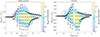Fig. 6. Combined results of combined dynamical ensemble calculation where the final states, plotted with black dots, are displayed against a background showing the 2D solar wind alpha particle and proton occurrence distributions. The final states are the same as those shown in Figures 3 and 5.

We combined the ensemble calculation results for both collisional relaxation and instability relaxation and display the outcome in Figure 6. We plot the final states with dots. The background shows the solar wind alpha particle (He⁺⁺) and proton occurrence distributions. We restate that the computation in the case of collisional relaxation was carried out up to Ω_pt = 2 × 10⁴, while for the instability-induced quasi-linear relaxation, the computation was carried out up to Ω_pt = 50.

4. Summary

In summary, this paper is an extension of our recent works (Yoon et al. 2024a,b) on the origin of the outer boundaries associated with the data distributions in (β_∥, T_⊥/T_∥) phase space. Our previous works (Yoon et al. 2024a,b), which are limited to proton and electron plasmas, have provided plausible explanations for the origin of these distributions by invoking the combined effects of collisions and instability excitation. In this paper, the same coupled mechanism is extended to include alpha particles (He⁺⁺), which dynamically couple to the protons. By carrying out ensemble simulations with the collisional dynamics and the instability-induced quasi-linear relaxation mechanism, we demonstrated that the combined effects provide a satisfactory explanation for the observed alpha particle and proton temperature distributions, thus resolving one of the long-standing problems in contemporary heliospheric physics.

The focus of the present paper is on the temperature anisotropies associated with the protons and alpha particles, but as we have noted previously, the protons and alpha particles are observed to possess a finite relative drift (see Figure 1). We did not take this feature into account, as the relative drift speed between the two species (normalized to Alfvén speed) is quite low, on the order of 𝒪(10⁻²). In the future, the effects of relative drift could be taken into consideration. We also restricted ourselves to the instabilities propagating in directions parallel (and anti-parallel) to the ambient magnetic field, but the influence of the obliquely propagating modes on the quasi-linear dynamics is an important subject that deserves a thorough consideration in the future. Even under the assumption of parallel propagation, we made an additional simplification in that the instabilities excited by particle temperature anisotropies can be treated as resonant types. These are the caveats of the present work that could be improved upon in the future. Despite the above-mentioned limitations, it is clear that the present paper provides a good first-cut explanation for the origin of both the high- and low-beta outer boundaries associated with the solar wind proton and alpha particle (He⁺⁺) data distributions.

Data availability

Movies associated with Figs. 3 and 5 are available at https://www.aanda.org

This paper deals with largely theoretical aspects, except for the solar wind proton and alpha particle (He⁺⁺) data that were used as the background. The data used in this project was accessed through the SPFD CDA Web service cdaweb.gsfc.nasa.gov. No new data are generated herewith.

Acknowledgments

This research was supported by NSF Grant 2203321 to the University of Maryland. This material is also based upon work funded by the Department of Energy (DE-SC0022963) through the NSF/DOE Partnership in Basic Plasma Science and Engineering. These results were also obtained (ML and SP) in the framework of the projects WEAVE project – G.0025.23N/FI 706/31-1 (FWO-Vlaanderen/DFG-Germany) and SIDC Data Exploitation (ESA Prodex-12). J.S. was supported by basic research funding from the Korea Astronomy and Space Science Institute (KASI2025185002). R.A.L. thanks the support of ANID, Chile, through Fondecyt grant No. 1251712. The authors have no conflicts to disclose.

References

Appendix A: Details of quasi-linear analysis

In the quasilinear theory of electromagnetic (proton and alpha) cyclotron and (parallel) firehose instabilities, it is necessary to solve the instantaneous dispersion relations, (16) and (17), to obtain the wave frequency as well as the instantaneous growth rates (18) and (19), at each time step during the numerical integration of the velocity moment equations (15). In the present paper we imposed an approximation scheme to obtain the complex frequency. Rather than a direct numerical solution, we made use of the cold-plasma dispersion relation to obtain the real frequency (see equations (16) and (17)) and the analytical growth rate based upon the assumption of resonant wave-particle interaction (see equations (18) and (19)). In the present Appendix, we first discuss the validity of the approximation by making direct comparisons against the exact numerical solutions of the transcendental dispersion equation. The dimensionless form of the exact dispersion relation (10) is given by

$$\begin{array}{c}\hfill 0=q^2\mp z-(1-2\delta )[A_{\pm }^p+{\eta }_{\pm }^{\mathit{pZ}}\left({\zeta }_{\pm }^p\right)]-\delta [A_{\alpha }+{\eta }_{\pm }^{\alpha }Z\left({\zeta }_{\pm }^{\alpha }\right)],\end{array}$$(A.1)

where ${\eta }_{\pm }^p$, ${\eta }_{\pm }^{\alpha }$, ${\zeta }_{\pm }^p$, and ${\zeta }_{\pm }^{\alpha }$ are defined in equation (9), or their normalized form in equation (15).

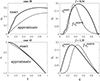Fig. A.1. Examples of exact versus approximate dispersion relations. [Top-left] real frequency and [top-right] growth rate for cyclotron instability (case 30). Solid curves are exact numerical solutions based upon equation (A.1), while the dashed curves are approximate solutions, equations (16) and (18), except that zi is multiplied by the scaling factor f = 0.305. [Bottom-left] Real frequency and [bottom-right] growth rate for firehose instability (case 43). Solid curves are exact numerical solutions based upon equation (A.1), while the dashed curves are approximate solutions based on equations (17) and (19), except that zi is multiplied by f = 1.35.

In Figure A.1 we display two sample cases of solutions, one corresponding to the proton-alpha particle system unstable to the excitation of left-hand cyclotron instability, namely case 30, and the other the system subject to the excitation of right-hand firehose mode instability, case 43. These two cases are chosen as representatives of the solar wind proton-alpha particle system that is sufficiently close to the marginal states of these instabilities. Shown on the top-left panel is the real frequency of the left-hand mode, while the top-right panel plots the corresponding growth rate. For case 30, the exact solution of equation (A.1) and the approximate solution based upon equations (16) and (18) are in qualitative agreement, but we also found that the approximate analytical growth rate is higher in absolute magnitude than the exact solution so that we adjusted the maximum growth rate of the approximate solution by a scaling factor f = 0.34. We found good agreement upon making an adjustment by multiplying the analytical growth rate by this scaling factor. The bottom-left and right panels are for case 43, for which the right-hand mode is unstable. As one may appreciate, the exact versus approximate real frequencies are in excellent agreement, while the growth rates also show reasonable agreement, provided the maximum growth rate computed from the analytical formula (19) is adjusted by a scaling factor f = 1.35. In this case, the analytical growth rate underestimates the actual growth rate.

We have found similarly reasonable agreements for other cases as well, provided the appropriate scaling factors are empirically determined. Table A.1 lists the scale factor, f, for each case, which we have compiled on the basis of an empirical method. In Table A.1, the number enclosed by the bracket is the initial ensemble position as indicated by Figure 4. Those ensemble points corresponding to stable conditions are indicated by S. Initial states that are unstable to either cyclotron or firehose instability excitation are indicated by the superscript C or F. We have multiplied the correction factors in the subsequent quasi-linear velocity moment ensemble calculations. While it is possible that the scaling/correction factor itself may evolve during the quasi-linear relaxation process, we have not varied f throughout the time evolution for the sake of simplicity.

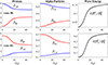Fig. A.2. Examples of quasi-linear velocity moments (macroscopic particle quantities) and wave energy density evolution. [Top-left] Proton betas, β⊥p and β∥p, versus Ωpt; [Top-middle] Alpha particle betas, β⊥α and β∥α, versus Ωpt; [Top-right] Wave energy density for the left-hand cyclotron mode, $\delta B_{-}^2/B_0^2={\displaystyle \int d}k\delta B_{-}^2(k)/B_0^2$, versus Ωpt, for case 30. [Bottom-left] Proton betas; [Bottom-middle] Alpha particle betas; [Bottom-right] Wave energy density for the right-hand firehose mode, $\delta B_{+}^2/B_0^2={\displaystyle \int dk}\delta B_{+}^2(k)/B_0^2$, versus Ωpt, for case 43.

In Figure A.2 we display sample results of quasi-linear velocity moments (that is, macroscopic particle quantities) as well as the total wave energy density, for the two reference cases, namely, cases 30 and 43. We have solved the normalized equations (15) up to Ω_pt = 50. For the descriptions of Figure A.2, we refer to the caption. As one can see from Figure A.2, proton betas as well as the wave energy density attain a quasi-saturated state by the time the system has evolved to Ω_pt = 50, but one may also notice that the alpha particle betas seem to be still evolving somewhat. Note that cases 30 and 43 are characterized by conditions not too far from the marginal stability states. As a result, it is not too surprising that the physical quantities have not completely reached the saturated states, as the instability growth rates are not very high. However, for systems far from the marginal stability conditions, we have found that the maximum collective instability saturation time of Ω_pt = 50 is sufficient to describe the quasi-linear relaxation process.

All Tables

All Figures

Fig. 1. [Left] Probability distribution function for nα/n versus nα/n, showing that the most probable value of nα/n is ∼𝒪(10−2). Those alpha particles satisfying the condition β∥α < 10−2, which turns out to be susceptible to collisional relaxation, are treated separately, and their partial probability distribution function is plotted with blue dots. The opposite condition β∥α > 10−2 turns out to define the solar wind condition susceptible to instability relaxation, and these alpha particles are treated separately. Their partial probability distribution function is plotted with red dots. [Right] Probability distribution function for |Vp − Vα|/VA versus the normalized proton-to-alpha relative drift speed, |Vp − Vα|/VA, showing that the most probable value of |Vp − Vα|/VA is also ∼𝒪(10−2).

In the text

	Fig. 2. [Left] Initial ensemble positions of alpha particles plotted against a background showing the alpha particle data distribution. [Right] Same but for the protons – and plotted against a backdrop showing the proton 2D distribution. The numerical designations signify the case numbers: 1 to 81.
In the text

	Fig. 3. [Left] Initial ensemble of alpha particle data points plotted with open circles. The dynamic paths in (β∥α, T⊥α/T∥α) space are indicated with magenta curves, and the final states at τmax = Ωptmax = 2 × 104 are marked with black dots. In the background is the alpha particle data distribution. [Right] Same but for the protons. (An associated movie is available online)
In the text

	Fig. 4. [Left] Initial ensemble positions in the case of collective instability relaxation – for alpha particles: plotted against a background showing the alpha particle data distribution. [Right] Same but for the protons – and plotted against a background showing the proton 2D distribution.
In the text

Fig. 5. [Left] Initial ensemble of alpha particle data points in the case of relaxation by instability excitation (plotted with open circles). The dynamic paths in (β∥α, T⊥α/T∥α) space are indicated with magenta curves and the final states at τmax = Ωptmax = 50 are marked with black dots. The background shows the alpha particle data distribution. [Right] Same but for the protons. An associated movie showing the entire dynamic paths for the ensemble points that are subject to instability excitation and quasi-linear relaxation is available online.

In the text

	Fig. 6. Combined results of combined dynamical ensemble calculation where the final states, plotted with black dots, are displayed against a background showing the 2D solar wind alpha particle and proton occurrence distributions. The final states are the same as those shown in Figures 3 and 5.
In the text

Fig. A.1. Examples of exact versus approximate dispersion relations. [Top-left] real frequency and [top-right] growth rate for cyclotron instability (case 30). Solid curves are exact numerical solutions based upon equation (A.1), while the dashed curves are approximate solutions, equations (16) and (18), except that zi is multiplied by the scaling factor f = 0.305. [Bottom-left] Real frequency and [bottom-right] growth rate for firehose instability (case 43). Solid curves are exact numerical solutions based upon equation (A.1), while the dashed curves are approximate solutions based on equations (17) and (19), except that zi is multiplied by f = 1.35.

In the text

Fig. A.2. Examples of quasi-linear velocity moments (macroscopic particle quantities) and wave energy density evolution. [Top-left] Proton betas, β⊥p and β∥p, versus Ωpt; [Top-middle] Alpha particle betas, β⊥α and β∥α, versus Ωpt; [Top-right] Wave energy density for the left-hand cyclotron mode, $\delta B_{-}^2/B_0^2={\displaystyle \int d}k\delta B_{-}^2(k)/B_0^2$, versus Ωpt, for case 30. [Bottom-left] Proton betas; [Bottom-middle] Alpha particle betas; [Bottom-right] Wave energy density for the right-hand firehose mode, $\delta B_{+}^2/B_0^2={\displaystyle \int dk}\delta B_{+}^2(k)/B_0^2$, versus Ωpt, for case 43.

In the text

References

- Alterman, B. L., & Kasper, J. C. 2019, ApJ, 879, L6 [Google Scholar]
- Alterman, B. L., Kasper, J. C., Stevens, M. L., & Koval, A. 2018, ApJ, 864, 112 [Google Scholar]
- Bale, S. D., Kasper, J. C., Howes, G. G., et al. 2009, Phys. Rev. Lett., 103, 211101 [NASA ADS] [CrossRef] [Google Scholar]
- Echeverría-Veas, S., Moya, P. S., Lazar, M., Poedts, S., & Asenjo, F. A. 2024, ApJ, 975, 112 [Google Scholar]
- Gary, S. P. 1993, Theory of Space Plasma Microinstabilities (Cambridge University Press) [Google Scholar]
- Huang, J., Kasper, J. C., Vech, D., et al. 2020, ApJS, 246, 70 [Google Scholar]
- Innocenti, M. E., Tenerani, A., & Velli, M. 2019, ApJ, 870, 66 [Google Scholar]
- Kasper, J. C., Lazarus, A. J., & Gary, S. P. 2002, Geophys. Res. Lett., 29, 1839 [Google Scholar]
- Kasper, J. C., Lazarus, A. J., Gary, S. P., & Szabo, A. 2003, Am. Inst. Phys. Conf. Ser., 679, 538 [Google Scholar]
- Kasper, J. C., Klein, K. G., Weber, T., et al. 2017, ApJ, 849, 126 [NASA ADS] [CrossRef] [Google Scholar]
- Klein, K. G., & Vech, D. 2019, RNAAS, 3, 107 [Google Scholar]
- Klein, K. G., Martinović, M., Standsby, D., & Horbury, T. S. 2019, ApJ, 887, 234 [NASA ADS] [CrossRef] [Google Scholar]
- López, R. A., Shaaban, S. M., & Lazar, M. 2021, J. Plasma Phys., 87, 905870310 [CrossRef] [Google Scholar]
- Maksimovic, M., Pierrard, V., & Lemaire, J. F. 1997, A&A, 324, 725 [NASA ADS] [Google Scholar]
- Maneva, Y. G., Ofman, L., & Viñas, A. 2015, A&A, 578, A85 [NASA ADS] [CrossRef] [EDP Sciences] [Google Scholar]
- Marsch, E., Zhao, L., & Tu, C. Y. 2006, Ann. Geophys., 24, 2057 [Google Scholar]
- Martinović, M. M., Klein, K. G., Ďurovcová, T., & Alterman, B. L. 2021, ApJ, 923, 116 [Google Scholar]
- Martinović, M. M., Klein, K. G., De Marco, R., et al. 2025, ApJL, 988, L25 [Google Scholar]
- Maruca, B. A., & Kasper, J. C. 2013, Adv. Space Res., 52, 723 [NASA ADS] [CrossRef] [Google Scholar]
- Maruca, B. A., Kasper, J. C., & Gary, S. P. 2012, ApJ, 748, 137 [NASA ADS] [CrossRef] [Google Scholar]
- Matteini, L., Landi, S., Hellinger, P., et al. 2007, Geophys. Res. Lett., 34, L20105 [Google Scholar]
- Micera, A., Zhukov, A. N., López, R. A., et al. 2020, ApJ, 903, L23 [NASA ADS] [CrossRef] [Google Scholar]
- Mostafavi, P., Allen, R. C., Jagarlamudi, V. K., et al. 2024, Front. Phys., 682, A152 [Google Scholar]
- Ofman, L., Viñas, A. F., & Maneva, Y. 2014, J. Geophys. Res. (Space Phys.), 119, 4223 [Google Scholar]
- Ofman, L., Yogesh, Boardsen, S. A., et al. 2025, ApJ, 984, 174 [Google Scholar]
- Ogilvie, K. W., Chornay, D. J., Fritzenreiter, R. J., et al. 1995, Space Sci. Rev., 71, 55 [Google Scholar]
- Pierrard, V., Lazar, M., & Schlickeiser, R. 2011, Sol. Phys., 269, 421 [NASA ADS] [CrossRef] [Google Scholar]
- Salem, C. S., Hubert, D., Lacombe, C., et al. 2003, ApJ, 585, 1147 [NASA ADS] [CrossRef] [Google Scholar]
- Salem, C. S., Pulupa, M., Bale, S. D., & Verscharen, D. 2023, A&A, 675, A162 [NASA ADS] [CrossRef] [EDP Sciences] [Google Scholar]
- Seough, J., Yoon, P. H., Nariyuki, Y., & Salem, C. 2023, ApJ, 953, 8 [Google Scholar]
- Shaaban, S. M., Lazar, M., Wimmer-Schweingruber, R. F., & Fichtner, H. 2021, ApJ, 918, 37 [NASA ADS] [CrossRef] [Google Scholar]
- Shaaban, S. M., Kennis, S., Lazar, M., Pierrard, V., & Poedts, S. 2025, J. Geophys. Res. Space Phys., accepted [Google Scholar]
- Short, B., Malaspina, D. M., Chasapis, A., & Verniero, J. L. 2024, ApJ, 975, 218 [Google Scholar]
- Štverák, Š., Trávníček, P., Maksimovic, M., et al. 2008, J. Geophys. Res. (Space Phys.), 113, A03103 [Google Scholar]
- Vafin, S., Riazantseva, M., & Pohl, M. 2019, ApJ, 871, L11 [NASA ADS] [CrossRef] [Google Scholar]
- Wilson, L. B., III, Stevens, M. L., Kasper, J. C., et al. 2018, ApJS, 236, 41 [NASA ADS] [CrossRef] [Google Scholar]
- Yoon, P. H. 2017, Rev. Mod. Plasma Phys., 1, 4 [NASA ADS] [CrossRef] [Google Scholar]
- Yoon, P. H., Seough, J., Hwang, J., & Nariyuki, Y. 2015, J. Geophys. Res., 120, 6071 [Google Scholar]
- Yoon, P. H., Lazar, M., Salem, C., et al. 2024a, ApJ, 969, 77 [NASA ADS] [CrossRef] [Google Scholar]
- Yoon, P. H., Salem, C. S., Klein, K. G., et al. 2024b, ApJ, 975, 105 [Google Scholar]