| Issue |
A&A
Volume 705, January 2026
|
|
|---|---|---|
| Article Number | L14 | |
| Number of page(s) | 8 | |
| Section | Letters to the Editor | |
| DOI | https://doi.org/10.1051/0004-6361/202557177 | |
| Published online | 12 January 2026 | |
Letter to the Editor
The near-infrared silhouette of the Flying Saucer edge-on disc revealed by the JWST JEDIce program
1
Institut des Sciences Moléculaires d’Orsay, CNRS, Univ. Paris-Saclay 91405 Orsay, France
2
Physique des Interactions Ioniques et Moléculaires, CNRS, Aix Marseille Université Marseille, France
3
Dept. Chemistry, University of California Berkeley CA, USA
4
Jet Propulsion Laboratory, California Institute of Technology 4800 Oak Grove Drive Pasadena CA 91109, USA
5
Astronomy Department, University of Virginia 530 McCormick Rd. Charlottesville VA 22903, USA
6
Institute of Astronomy, Department of Physics, National Tsing Hua University Hsinchu, Taiwan
7
Leiden Observatory, Leiden University Leiden, The Netherlands
8
Center for Astrophysics, Harvard & Smithsonian 60 Garden St. Cambridge MA 02138, USA
9
Astrophysics & Space Institute, Schmidt Sciences New York NY 10011, USA
10
Physikalisch-Meteorologisches Observatorium Davos und Weltstrahlungszentrum Dorfstrasse 33 7260 Davos Dorf, Switzerland
11
Univ. Grenoble Alpes, CNRS, IPAG 38000 Grenoble, France
12
Star and Planet Formation Laboratory 2-1 Hirosawa Wako Saitama 351-0198, Japan
★ Corresponding author: This email address is being protected from spambots. You need JavaScript enabled to view it.
Received:
9
September
2025
Accepted:
15
December
2025
Abstract
Aims. Edge-on discs offer a unique opportunity to probe radial and vertical dust and gas distributions in the protoplanetary phase. This study aims to investigate the distribution of micron-sized dust particles in the Flying Saucer in Rho Ophiuchi by leveraging the unique observational conditions of a bright infrared background that enables the edge-on disc to be seen in both silhouette and scattered light at specific wavelengths.
Methods. We used NIRSpec IFU observations from the JWST Edge-on Disc Ice program (JEDIce) of the Flying Saucer serendipitously observed against a Polycyclic Aromatic Hydrocarbons-emitting background to constrain the dust distribution and grain sizes via radiative transfer modelling.
Results. The observation of the Flying Saucer in silhouette at 3.29 μm reveals that the midplane radial extent of small dust grains is ∼235 au, i.e. larger than the large-grain disc extent previously determined to be 190 au from millimetre data. The scattered light observed in emission probes micron-sized icy grains at large vertical distances above the midplane. The vertical extent of the disc silhouette is similar at visible, near-IR, and mid-IR wavelengths, corroborating the conclusion that dust settling is inefficient for grains as large as tens of microns, both vertically and radially.
Key words: radiative transfer / scattering / solid state: volatile / planets and satellites: formation / protoplanetary disks / dust, extinction
© The Authors 2026
 Open Access article, published by EDP Sciences, under the terms of the Creative Commons Attribution License (https://creativecommons.org/licenses/by/4.0), which permits unrestricted use, distribution, and reproduction in any medium, provided the original work is properly cited.
This article is published in open access under the Subscribe to Open model. This email address is being protected from spambots. You need JavaScript enabled to view it. to support open access publication.
1. Introduction
Protoplanetary discs with an ‘edge-on’ viewing geometry are oriented with the disc occulting the star along our line of sight and thus provide a unique view of the disc’s vertical structure (e.g. Burrows et al. 1996; Watson et al. 2007; Lin et al. 2023; Duchêne et al. 2024; Dartois et al. 2025; Ballering et al. 2025). The ‘Flying Saucer’ edge-on disc (BKLT J162813-243139) was discovered at the periphery of the ρ Ophiuchi cloud complex in the near-infrared (J, H, and Ks bands) by Grosso et al. (2001, 2003). In the millimetre wavelength, this edge-on disc appears in silhouette against the CO J = 2−1 emission from the background ρ Oph molecular cloud complex Guilloteau et al. (2016). From these near-IR to millimetre studies, the inclination of the Flying Saucer is estimated to be i ≳ 86°. Using Spitzer mid-IR spectroscopic data and additional near-IR and mid-IR photometric constraints, Pontoppidan et al. (2007) found that including large grains up to ten micrometres in size in the disc surface layers was required to explain the scattered light level in the spectral energy distribution for this disc. In this letter, we focus on the newly revealed near-IR silhouette of the Flying Saucer disc, which is – at some wavelengths – observed both in emission and extinction by JWST NIRSpec. In Sect. 2, we summarise the observations and the specific wavelengths where the disc appears in absorption against the background. In Sect. 3 we present radiative transfer models of dust grain distributions and the structure of the disc in order to compare it with the observations. We discuss the implications for the disc’s dust sizes and settling in Sect. 4.
2. Observations
The observations presented here are part of the JWST Edge-on Disc Ice program (JEDIce, GO #5299, PI J. Bergner). The Flying Saucer (BKLT J162813-243139) was observed with NIRSpec on August 25, 2024. The observations were taken with the G235H and G395H filters from 1.66–3.17 μm and 2.87–5.27 μm, respectively, at a spectral resolution of R ∼ 2700 using the IFU observing mode with a pixel scale of 0.1″ pixel−1 and a field of view of 3″ × 3″. A two-tile mosaic was used to capture the full extent of the disc. For both the G235H and G395H observations, we used a small cycling dither pattern with 12 points and the NRSIRS2RAPID readout pattern. Twenty-five (ten) groups per integration were used for the G395H (G235H) observations for a total exposure time of 4552 (1926) sec. Data were reduced using calibration software version 1.17.1 and reference file database jwst_1322.pmap. The Flying Saucer disc, which lies at the edge of the ρ Oph cloud complex, is surrounded by an extended ambient emission field of infrared fluorescence (Leger & Puget 1984) from Astronomical Polycyclic Aromatic Hydrocarbons (astro-PAH) carriers exposed to ultraviolet photons. Within the NIRSpec cube, the disc is observed not only via the scattered light from its upper layers but also in extinction close to the disc midplane at the characteristic wavelengths corresponding to strong PAH emission features. This is particularly evident at around 3.29 μm, as shown in Fig. 1. A second object, most likely a field star, can be seen in the NE of the field and is not considered hereafter. We complemented the NIRSpec data with archive data spanning the visible to the millimetre range. We retrieved archival data from the Hubble Space Telescope (HST; F475W, 0.47 μm, program #13643), JWST MIRI/Imager (F770W, 7.7 μm, program #4290), and JWST MIRI/MRS (Channel 3, program #1280), in which the disc is also seen in extinction against a background of astro-PAH or H2 emission. We also included ALMA Band 7 continuum data (cycle 9 program #2022.1.00742.S), in which the disc is observed in emission. For the JWST MIRI/MRS datacube, three imaging frames were stacked around the peak of the H2 line at 17.035 μm to reproduce a narrow band imaging filter. These archive images are shown in Fig. A.1.
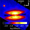 |
Fig. 1. NIRSpec spectroscopic imaging data at 3.29 ± 0.015 μm (i.e. stacking channels at the peak of the PAH band). The disc is observed both in emission (lobes, red-yellow) and in silhouette (midplane, black) against the ambient field emission arising from the CH stretching mode of UV-excited astro-PAHs (blue). |
The 17.035 μm synthetic narrow band filter provides an important constraint because it is the longest wavelength with little or no dust settling at which the disc silhouette is observed, as is shown below. The HST and JWST wideband imaging observations provide additional information, though they are limited by the fact that the signal from the various contributing components is integrated across the whole filter bandwidth. We used the broadband images at 7.7 μm and in the millimetre to show the continuity in the mid-IR and compare near-to-mid-IR JWST to the observed millimetre dust settling, respectively. The focus of our analysis is on narrow band images derived from the NIRSpec spectro-imaging datacube (see Appendix B). These data provide snapshots of the disc continuum emission at reference wavelengths where the ambient emission field is weak and the silhouette of the disc is seen in extinction against this continuum at nearby wavelengths. The images constrain the disc model.
3. Modelling the Flying Saucer
To better understand the NIRSpec observations and reproduce the wavelength dependence in the observed images, we described the Flying Saucer with a radiative transfer model using the RADMC-3D1 software (Dullemond et al. 2012). The modelling applied to this disc uses the same framework and parameter definitions as previously described for the benchmark model of the edge-on disc Tau 042021 in Dartois et al. (2025) and in Appendix C. For the Flying Saucer model, two additional components are required: (i) an external field to simulate the extended ambient astro-PAH emission field and (ii) a foreground extinction. Two icy grain populations are required: a small-grain population of sizes 0.005 to 10 μm with an external midplane radius of rout = 235 au and a settled-grain population of 15–3000 μm with an external midplane radius of  au. This
  matches the value reported by Guilloteau et al. (2016, 2025). The final model images are presented and interpreted following radiative transfer, ray tracing, and convolution with beam Point Spread Functions (PSFs).
4. Constraints on the disc size and dust properties
The model of the Flying Saucer exhibits a very good overall agreement with the observational spectral imaging, as can be seen in Fig. 2, where we present the model convolved to the JWST spatial resolution via application of the PSF. The overall shapes and intensities of the lobes and the extincted disc midplane are well reproduced. The full resolution model is shown on a one colour scale in Appendix D.
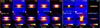 |
Fig. 2. Benchmark model of the Flying Saucer from near-IR to millimetre compared to observations on a 5″ × 5″ field of view. The upper row shows the model images, convolved to observed spatial resolutions, and the bottom row displays the observations. Selected wavelengths across the NIRSpec range are shown along with archival images at 7.639 μm (MIRI/Imager F770W filter pivot wavelength), 17.035 μm (MIRI/MRS), and millimetre (ALMA) wavelengths. The contribution of the H2 disc wind at 3.004 and 17.035 μm was not included in the model. The components dominating the ambient emission field at each wavelength are labelled astro-PAH and H2 on the corresponding images. Images were rotated by 3° to account for the position angle. |
The 7.7 μm MIRI archival image, included for completeness in Fig. 2, shows much stronger background continuum emission than what appears at the lower wavelengths measured by NIRSpec. We determined spectroscopically that the emission from astronomical PAHs dominates the emission field at ∼3.29 μm (Fig. B.1) and therefore must also contribute emission in the ∼8 μm region. In addition, it is probable that the 7.7 μm emission field contains a continuum contribution from very small dust particles in the Ophiuchi cloud complex, as recorded in Spitzer IRAC band 4 images at 8 μm (Evans et al. 2009). In wavelength ranges covered only by photometric observations (e.g. ∼8 μm) the model is slightly less accurate, given that further components (i.e. atomic or molecular lines) may possibly also be contributing an unknown fraction of the flux captured by the F770W filter. Spectroscopy would be required to disentangle the various components. Nevertheless, for the ambient field adopted in the model (Fig. B.2), we obtained agreement with the observation, including the distinct silhouette extinction pattern near the midplane. To precisely characterise the disc extinction, we produced high-contrast images via synthetic imaging filters. The second column in Fig. 2 is centred on the ambient emission from a narrow rovibrationally excited H2 line (at 3.004 μm). Despite its low signal-to-noise ratio, the disc is clearly detected in silhouette along the midplane, with the continuum of the emission line corresponding to a maximum of a wide water ice absorption band (see Appendix B). In another wavelength region of interest, one filter is centred on the maximum of the PAH emission feature at 3.29 μm (filter I3.29, stacking images within 3.29 ± 0.01 μm), and another is centred just before the rise of the PAH stretching mode at 3.2 μm (filter I3.2, stacking all images within 3.2 ± 0.01 μm; Fig. B.1). The images are shown in the upper panels of Fig. 3. By dividing  , where
  is the flux level in the surrounding ambient field from astro-PAHs, we corrected for the disc scattered light and isolated the observed extinction silhouette (τ = −ln(T)), shown in the upper-right panel of Fig. 3. The model reproduces the disc’s vertical and horizontal profiles well, both in terms of the apparent optical depth profile along the midplane and the outer radius of the silhouette disc (Fig. 3).
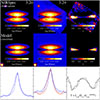 |
Fig. 3. Observations and models of disc emission and silhouette. Left and centre columns show the emission at 3.2 μm (I3.2, no astro-PAH background) and 3.29 μm (I3.29, peak astro-PAH background), respectively. The right column shows the extincted optical depth |

The detection of the disc in extinction offers an opportunity to directly probe the extent of the Flying Saucer midplane. For comparison, our observations are plotted over ALMA band 7 continuum data in Fig. 4. Using a combination of several ALMA datasets, a large-grain disc size of ∼190 au was recently measured in Guilloteau et al. (2025). It is clear that the disc midplane measured in extinction at 3.29 μm by NIRSpec has a larger extent compared to the millimetre disc measured by ALMA. When comparing the NIRSpec data to archival images of the extincted disc measured at 0.47 μm (HST) and 7.7 μm (MIRI), all three also exhibit a similar spatial extent, corresponding to a radius of about 235 ± 10 au (for an adopted distance of 120 pc).
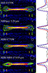 |
Fig. 4. Silhouette of the Flying Saucer disc seen against the ambient field at different wavelengths (green contours) plotted over the ALMA Band 7 millimetre dust disc image (colour map). From top to bottom, the disc silhouette is shown at 0.47 (HST F475W), 3.29 (NIRSpec), 7.7 (MIRI F770W), and 17.035 (MIRI/MRS) microns. Image and contours are rotated by 3°. The image is 5″ wide. In each panel, two sets of vertical tick marks denote the outer radii determined in the model for the small grain (235 a.u., green) and large grain (190 a.u., orange) populations, assuming a distance of 120 pc. The full width half maximum of the PSFs are shown as circles. At each wavelength, normalised vertical profiles are plotted to the right of the image. These are the projection across the full disc diameter for the ALMA image (dot-dashed, black) and cuts taken through the thickest point of the left lobe of the silhouette (red) and right lobe of the silhouette (blue). In the radial and vertical directions, the disc silhouette clearly has a greater extent than the continuum image. |
In addition to the larger horizontal extent, it is clear that the vertical extent of the extincted disc measured by NIRSpec is also larger than that measured by ALMA. Note that for this comparison, we focused on the outer radial region of the disc. The silhouette (extinction) has a dumbbell shape since the contribution of disc scattering and emission prevents us from measuring the disc extent towards the inner radial region. These observations together clearly show that the grains probed across the entire visible to mid-IR range, spanning sub-micron to tens of micron sizes, are not settled to a large extent; in agreement with the full radiative transfer model we present in this work; and contrary to the larger grains probed with ALMA. Interestingly, in our dust model, the small-grain scale height at 100 au (about 7.8 au) is lower than that required to model observations of gas phase ALMA CO (2-1) transitions (13.5 au at 100 au; Guilloteau et al. 2025; Dutrey et al. 2025, taking into account the factor difference in parametrisation). In our model, the small-grain distribution primarily traces icy dust grains. The right panel of Fig. B.1 shows the presence of water ice at high vertical altitude in the disc, especially in the upper lobe, thus requiring that icy grains are used up to high altitude in the radiative transfer model of this disc. This would correspond to elevations where the gas phase CO depletion begins in Guilloteau et al. (2025), i.e. the onset of H2O/CO ice (snow) surfaces. In contrast, some millimetre CO transitions may be probing the more extended atmosphere, which deviates from a Gaussian hydrostatic profile and dominates at large scale heights. This explains why we also require the inclusion of a small fraction of the disc’s small-grain dust population at very high elevations (see the parameters in Appendix C). It should be noted that some of the parameters in such disc models could be interconnected, e.g., changing the surface density exponent parameter p will influence the scale height exponent parameter h while still providing an acceptable fit.
The large-grain scale height in our model is only about a third or a quarter as large as the small-grain scale height, signifying a settling of millimetre-sized grains to the midplane. We find that the small-grain population responsible for most of the near-IR to mid-IR emission component requires grains up to at least 10 μm in size, in agreement with Pontoppidan et al. (2007). This lends further evidence that the dust grains up to tens of microns in size are not settled, contrary to the (sub)-millimetre grains, which helps constrain the role of turbulence and vertical mixing in discs (Villenave et al. 2020; Sturm et al. 2024; Duchêne et al. 2024; Dartois et al. 2025; Tazaki et al. 2025).
Overall, the possibility of comparing highly spatially resolved JWST observations of dust, gas, and ice to those obtained by instruments spanning wavelengths from the visible to the millimetre currently offers a comprehensive vision of complex phenomena in discs, constraining, for example, the spatial extent of cavities (Sturm et al. 2024), nested small dust grain and gas outflows (Duchêne et al. 2024; Dartois et al. 2025), and dust settling (Villenave et al. 2020) or condensation (McClure et al. 2025) and tracing disc silhouettes (Ballering et al. 2025). These new JWST observations of Flying Saucer unambiguously reveal the small-grain disc extent in silhouette against an ambient astro-PAH background. The silhouette disc is also seen in extinction against vibrationally excited H2 emission, although at a lower signal-to-noise ratio. The detection of the disc in extinction offers a rare opportunity to directly probe the full horizontal extent of the disc without relying on scattered light. The silhouette disc extends to larger radii than the large grains observed by ALMA, thus providing complementary constraints on the overall disc structure and grain settling behaviour. We observed a distinctive dumbbell shape of the silhouette disc, which reflects the vertical extent of the small-grain population. The similarity of the silhouette disc shape across visible to mid-IR wavelengths confirms that grains up to tens of microns in size are not settled, even as far out as the disc outer truncation radius. Follow-up analysis will be performed to retrieve the full potential of this dataset, including finer spectroscopic exploration.
Acknowledgments
This work is based on observations made with the NASA/ESA/CSA James Webb Space Telescope and the NASA/ESA Hubble Space Telescope. The data were obtained from the Mikulski Archive for Space Telescopes at the Space Telescope Science Institute, which is operated by the Association of Universities for Research in Astronomy, Inc., under NASA contracts NAS 5–26555 and NAS 5-03127. The specific observations analyzed can be accessed via https://doi.org/10.17909/w4sg-d032. Support for Program number 5299 was provided by NASA through a grant from the Space Telescope Science Institute, which is operated by the Association of Universities for Research in Astronomy, Inc., under NASA contract NAS 5-03127. This paper also makes use of data from the ALMA program 2022.1.00742.S. ALMA is a partnership of ESO (representing its member states), NSF (USA) and NINS (Japan), together with NRC (Canada), NSTC and ASIAA (Taiwan), and KASI (Republic of Korea), in cooperation with the Republic of Chile. The Joint ALMA Observatory is operated by ESO, AUI/NRAO and NAOJ. ED and JAN acknowledge support from the Thematic Action ‘Physique et Chimie du Milieu Interstellaire’ (PCMI) of INSU Programme National ‘Astro’, with contributions from CNRS Physique & CNRS Chimie, CEA, and CNES. JCS is supported by the Heising-Simons Foundation through a 51 Pegasi b Fellowship. ZYL is supported in part by NASA 80NSSC20K0533 and NSF AST-2307199. LM, FMe, received funding from the European Research Council (ERC) under the European Union’s Horizon Europe research and innovation program (grant agreement No. 101053020, project Dust2Planets). Part of this research was carried out at the Jet Propulsion Laboratory, California Institute of Technology, under a contract with the National Aeronautics and Space Administration (80NM0018D0004).
References
- Ballering, N. P., Cleeves, L. I., Boyden, R. D., et al. 2025, ApJ, 979, 110 [Google Scholar]
- Burrows, C. J., Stapelfeldt, K. R., Watson, A. M., et al. 1996, ApJ, 473, 437 [Google Scholar]
- Compiègne, M., Verstraete, L., Jones, A., et al. 2011, A&A, 525, A103 [Google Scholar]
- Crameri, F., Shephard, G. E., & Heron, P. J. 2020, Nat. Commun., 11, 5444 [NASA ADS] [CrossRef] [Google Scholar]
- Dartois, E., Noble, J. A., Ysard, N., Demyk, K., & Chabot, M. 2022, A&A, 666, A153 [NASA ADS] [CrossRef] [EDP Sciences] [Google Scholar]
- Dartois, E., Noble, J. A., McClure, M. K., et al. 2025, A&A, 698, A8 [NASA ADS] [CrossRef] [EDP Sciences] [Google Scholar]
- Draine, B. T. 2003, ARA&A, 41, 241 [NASA ADS] [CrossRef] [Google Scholar]
- Duchêne, G., Ménard, F., Stapelfeldt, K. R., et al. 2024, AJ, 167, 77 [CrossRef] [Google Scholar]
- Dullemond, C. P., Juhasz, A., Pohl, A., et al. 2012, RADMC-3D, Astrophysics Source Code Library [record ascl:1202.015] [Google Scholar]
- Dutrey, A., Denis-Alpizar, O., Guilloteau, S., et al. 2025, A&A, 704, A33 [NASA ADS] [CrossRef] [EDP Sciences] [Google Scholar]
- Evans, N. J., II, Dunham, M. M., Jørgensen, J. K., et al. 2009, ApJS, 181, 321 [Google Scholar]
- Grosso, N., Alves, J., Neuhäuser, R., & Montmerle, T. 2001, A&A, 380, L1 [NASA ADS] [CrossRef] [EDP Sciences] [Google Scholar]
- Grosso, N., Alves, J., Wood, K., et al. 2003, ApJ, 586, 296 [Google Scholar]
- Guilloteau, S., Piétu, V., Chapillon, E., et al. 2016, A&A, 586, L1 [NASA ADS] [CrossRef] [EDP Sciences] [Google Scholar]
- Guilloteau, S., Denis-Alpizar, O., Dutrey, A., et al. 2025, A&A, 700, L5 [NASA ADS] [CrossRef] [EDP Sciences] [Google Scholar]
- Leger, A., & Puget, J. L. 1984, A&A, 137, L5 [Google Scholar]
- Lin, Z.-Y. D., Li, Z.-Y., Tobin, J. J., et al. 2023, ApJ, 951, 9 [NASA ADS] [CrossRef] [Google Scholar]
- McClure, M. K., van’t Hoff, M., Francis, L., et al. 2025, Nature, 643, 649 [Google Scholar]
- Pontoppidan, K. M., Stapelfeldt, K. R., Blake, G. A., van Dishoeck, E. F., & Dullemond, C. P. 2007, ApJ, 658, L111 [CrossRef] [Google Scholar]
- Sturm, J. A., McClure, M. K., Harsono, D., et al. 2024, A&A, 689, A92 [NASA ADS] [CrossRef] [EDP Sciences] [Google Scholar]
- Tazaki, R., Ménard, F., Duchêne, G., et al. 2025, ApJ, 980, 49 [Google Scholar]
- Villenave, M., Ménard, F., Dent, W. R. F., et al. 2020, A&A, 642, A164 [EDP Sciences] [Google Scholar]
- Watson, A. M., Stapelfeldt, K. R., Wood, K., & Ménard, F. 2007, in Protostars and Planets V, eds. B. Reipurth, D. Jewitt, & K. Keil, 523 [Google Scholar]
Appendix A: Archive data
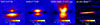 |
Fig. A.1. Archival data showing the disc in broadband imaging from HST (visible, extinction), JWST MIRI/Imager (mid-IR, extinction), and ALMA (Band 7, emission) and a narrowband filter derived from spectro-imaging with JWST MIRI/MRS (mid-IR, extinction). |
Appendix B: Adopted external ambient field
The illuminating external ambient field in our model in the NIRSpec wavelength range is derived directly from JWST observations well away from the disc. Physically, this field is the result of emission from the astro-PAH component in the nearby cloud. Details of the footprint used are shown in Fig.B.1(left). This figure also show that the CH stretching mode emission observed in the image is not arising from the disc itself by comparing the total flux in the image to a footprint enclosing the disc emission (middle). The right panel of Fig.B.1 displays the apparent optical depth observed by comparing the images at the maximum extinction level in the water ice OH stretching mode band at 3.05 μm to a reference channel in the adjacent continuum at 3.6 μm (filters shown in dark blue in the middle panel of Fig.B.1 and constructed using channels around 3.05 and 3.6 μm), by forming the optical depth image (−ln(I3.05/I3.6)). The optical depth image clearly show the presence of water ice absorption at high vertical altitude in the disc, especially in the upper lobe, requiring icy grains to model the disc radiative transfer.
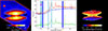 |
Fig. B.1. External ambient field extraction and icy grains water ice extinction map. Left: Footprints used to extract (i) the disc emission (blue contour) and (ii) the flux in the entire image (red contour). The ambient field contribution is derived by subtracting one from the other. Middle: Spectrum of the entire field (red), spectrum within the disc footprint (blue), and difference spectrum to show the ambient emission field (green). The vertical filled regions show the bandpasses of the tailored filters, which were used to make the images shown in Fig.2 (light blue, at (2.99 and 3.02), 3.2, and 3.29 μm). For the H2 image at 3.004 μm, only the three channels in which the emission line contributes were used (around the position shown with the magenta arrow), whereas the emission line-free filter, termed ‘2.99 μm’, makes use of the channels on both sides of the line position to estimate the disc emission around this H2 line. Right: Optical depth image (−ln(I3.05/I3.6)) made using the two filters shown in dark blue in the middle panel and constructed using channels around 3.05 and 3.6 μm. The optical depth image clearly shows the presence of water ice extinction (OH stretching mode absorption at 3.05 μm) at high vertical altitude in the disc, especially in the upper lobe, requiring icy grains to model the disc radiative transfer. |
In the mid-IR range, in the absence of more spectral information, we scaled the expected contribution by astronomical PAHs to reach the ∼12MJy/sr intensity in the continuum in the F770W MIRI filter, as shown in Fig. B.2. A more detailed ambient field would require spectral information to be able to measure the continuum contribution from very small grains on top of which the contribution of the astronomical PAH mid-IR bands would lie.
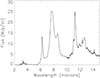 |
Fig. B.2. Ambient field adopted in the modelling. The near-IR (2.9–4 μm) region was directly obtained from NIRSpec observations in this work (see Fig.B.1). The mid-IR part (5.5-15 μm) is a Spitzer spectrum, measured around the disc HD97300, whose flux was scaled to mimick the expected ISRF flux in the 7.7 μm JWST broadband filter. In the mid-IR, the contribution to an underlying continuum from the emission of very small grains (e.g. Compiègne et al. 2011) would be required to derive a more accurate ambient field emission profile. |
Appendix C: Benchmark disc model
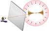 |
Fig. C.1. Schematic view of the Flying Saucer radiative transfer calculation. The disc is immersed in an external astro-PAH ambient emission field modelled as a spheroidal envelope, illustrated in red, and lies behind a foreground extinction, illustrated in grey. |
The best-fit benchmark model we obtained is shown in Fig.2. This model reproduces the spatial distribution in emission and extinction from the near-IR to the millimetre. The definition of all model parameters and their values in the benchmark model are given here. A schematic view of the different model components used to model the Flying Saucer is shown in Fig.C.1. For a close-up of the disc grain spatial distribution scheme, we refer to the benchmark model of Fig.5 in Dartois et al. (2025). The external field spectrum was estimated in the NIRSpec range by summing sky spaxels in the external continuum around the Flying Saucer, and is shown in Fig.B.1. It was extended into the mid-IR (Fig.B.2) using the astronomical PAH emission band spectrum of the HD97300 disc retrieved from the Spitzer archive (PID 2; Astronomical Observation Request 12697088, Low and High resolution). This Mid-IR spectrum was scaled to achieve an integrated flux compatible with (i) the MIRI F770W region outside of the disc, and (ii) the archival IRAC 8 μm filter extended maps of the Spitzer legacy program c2d Evans et al. (2009). In addition, as discussed previously in the pioneering work on this source from Grosso et al. (2003), a foreground interstellar dust extinction must be taken into account. For this extinction contribution, we added an RV = 5.5 Milky Way extinction curve taken from Draine (2003), adjusted to the expected visual extinction of around AV= 2.
To analyse the observations, we use a benchmark disc model with several layers of structural complexity as described below. The classical, so-called ‘standard’ disc model making the core of the model is based on an axisymmetric flaring disc around a young star, described using classical parameters. The surface density of the disc is parametrised with
 (C.1)
(C.1)
where r is the radial distance to the star, r0 is a reference radius and Σ0 the surface density normalisation at this reference radius. p is the power law exponent describing the radial variation, positive if the surface density decreases with radius. The density is tapered by an exponential edge with reference radius rt, following the viscous disc model theoretical solution (Lynden-Bell & Pringle 1974).
The vertical density distribution, under hydrostatic equilibrium, is given by
 (C.2)
(C.2)
with the density at radial distance r and vertical distance z from the midplane, and where H(r) is the vertical scale height under a vertical isothermal hypothesis, whose radial variation is given by
 (C.3)
(C.3)
where H0 is the scale height at the reference radius r0. h is the power law exponent describing the scale height radial variation, > 1 for flaring discs. The midplane density radial variation thus evolves with a power law as s = −(p + h).
The disc extends from its inner radius rin, defined by the sublimation temperature of the refractory components to the outer radius rout. The large grain distribution possesses its own (lower) scale height  .
.
To model the effect of an extended atmosphere, i.e. an atmosphere deviating from the pure hydrostatic equilibrium, we adopt a simple configuration by slightly modifying the vertical density profile in a way which allows empirically fitting some of the protoplanetary disc expected prescriptions models, some cited in Dartois et al. (2025).
To do so, above a given altitude, the extended atmosphere takes precedence over the classical hydrostatic decay, and is defined by parameters ϵ and η. We thus modified Eq. C.2 by replacing it with the following extended atmosphere equation:
 (C.4)
(C.4)
The transition where Eq. C.2 equals Eq. C.4 occurs at
 (C.5)
(C.5)
To obtain the benchmark model fit shown in this study, we used a  minimisation scheme simultaneously minimising the sum of several reduced
  s, taking into account the following major constraints: the log intensity of the observed image at 3.29 μm, the silhouette cuts along the midplane at 3.29 and 7.7 μm, the cut along the midplane after dividing the 3.29 μm image by 3.2 μm image, as shown in Fig.3, and the fluxes of the different images. This minimisation scheme provides a balance of all these different observational constraints. The minimisation was performed using a Nelder-Mead downhill simplex method algorithm, starting from various initial conditions within the parameter space provided to the algorithm to verify that the final result is not a local minimum. The parameter space exploration was made over the following ranges: inclination = 86°−89°, hydrogen number density at the reference radius r0 of 100 au, nH2(100 au) = 107 − 5 × 108 cm−3, p = 0.0−1.0, rin = 0.07-10 au, rout = 200-250 au, H0 = 4−13 au, h = 1.0−1.5,
  . The grain size distribution boundaries (amin, amax, a
 , a
, a ) were explored on a discrete grid: 0.005, 0.1, 0.3, 0.7, 1, 2, 3, 5, 10, 15, 20, 30, 40, 50, 60, 100, 1000, and 3000 μm.
The main parameters of the benchmark RADMC3D model shown in the article are: Tstar = 3700 K, a disc inclination of 87.8°, the hydrogen number density, at the reference radius r0 of 100 au, nH2(100 au) = 1.05 × 108 cm−3, p = 0.23, rin = 0.07 au, rout = 235 au, H0 = 7.8 au, h = 1.23,  au. The NIRSpec instrumental PSF is on the order of 0.1″ around 3 μm, corresponding to the ±∼10 au reported in the main text. The model includes the possibility to include a lower density cavity rcav. The model result with rcav = 1.05 au agrees well with the recent study probing large grains with ALMA (< 2 au, Guilloteau et al. 2025).
Among the salient parameters of this model is the need for two grain size distributions: a small-grain population ranging in size from amin = 0.005 μm to amax = 10 μm and extending to an external midplane radius of rout = 235 au; and a settled-grain population ranging from a = 15 μm to a
 = 3000 μm and extending to an external midplane radius of
  = 190 au. The ice used for the grain mantles is a H2O:CO2:CO:NH3 mixture; optical constants are given in Dartois et al. (2022). The settled large grain scale height in this model (
 = H0/4.5) corresponding to the ALMA Band 7 image. Such a settling factor can be considered as ‘moderate’ when compared to other evolved discs (e.g. Villenave et al. 2020), most probably because in the Flying Saucer disc, as suggested by Guilloteau et al. (2025), the host star is still relatively young, which explains their finding of an H0 ∼ 6 au in the millimetre, based on a more complete millimetre observations coverage, and considering an exponent of less than unity which implies some tapering in the outer disc. The extended atmosphere, which extends the small grains distribution’s vertical presence above the classical hydrostatic density decay, is calculated with set parameters ϵ = 2.5 and η = 1.0.
Appendix D: Models on a one-colour scale
This appendix contains the full benchmark model including the model images presented at full calculated resolution i.e. prior to being convolved by the instrumental Point Spread Function at the corresponding wavelengths (Fig.D.1, upper row). As discussed in many articles such as Crameri et al. (2020), the use of appropriate colour scales and the addition of a colour bar is mandatory to be able to interpret what is modelled without distorting the perception of the image, as well as to allow colour visually deficient people, amounting to a significant fraction of the population, to perceive the scales in the same way. To this end, we provide the models coded with two colour palettes, providing the one colour scale version in this appendix. Both colour palettes chosen should be close to being perceptually uniform. In the same effort, we systematically added colour bars for the reader to refer to.
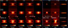 |
Fig. D.1. Benchmark model of the Flying Saucer from near-IR to millimetre compared to observations on a 5″ × 5″ field of view. The central and lower rows present the same data as Fig. 2 but on a single colour scale. The upper row presents the non-convolved, full resolution model images. |
Appendix E: Effect of resolution on apparent optical depth in the dark lane
In Fig. 3 we show horizontal cuts through the observations and PSF-convolved models that compare, at the same spatial resolution, the apparent optical depth along the midplane of the disc. This appears to be concentrated/located in two lobes near the outer disc whereas at small stellocentric radius, the apparent optical depth increases because of beam dilution which merges scattered light from the disc lower local scale height. Here, we present a comparison with the full resolution model cut, to illustrate that higher angular resolution observations would reveal a consistently deeper apparent optical depth across the midplane close to the star, whereas it asymptotically converges towards the observed depth at large stellocentric radius.
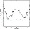 |
Fig. E.1. Midplane cut for |
All Figures
|
Fig. 1. NIRSpec spectroscopic imaging data at 3.29 ± 0.015 μm (i.e. stacking channels at the peak of the PAH band). The disc is observed both in emission (lobes, red-yellow) and in silhouette (midplane, black) against the ambient field emission arising from the CH stretching mode of UV-excited astro-PAHs (blue). |
| In the text | |
|
Fig. 2. Benchmark model of the Flying Saucer from near-IR to millimetre compared to observations on a 5″ × 5″ field of view. The upper row shows the model images, convolved to observed spatial resolutions, and the bottom row displays the observations. Selected wavelengths across the NIRSpec range are shown along with archival images at 7.639 μm (MIRI/Imager F770W filter pivot wavelength), 17.035 μm (MIRI/MRS), and millimetre (ALMA) wavelengths. The contribution of the H2 disc wind at 3.004 and 17.035 μm was not included in the model. The components dominating the ambient emission field at each wavelength are labelled astro-PAH and H2 on the corresponding images. Images were rotated by 3° to account for the position angle. |
| In the text | |
|
Fig. 3. Observations and models of disc emission and silhouette. Left and centre columns show the emission at 3.2 μm (I3.2, no astro-PAH background) and 3.29 μm (I3.29, peak astro-PAH background), respectively. The right column shows the extincted optical depth |
| In the text | |
|
Fig. 4. Silhouette of the Flying Saucer disc seen against the ambient field at different wavelengths (green contours) plotted over the ALMA Band 7 millimetre dust disc image (colour map). From top to bottom, the disc silhouette is shown at 0.47 (HST F475W), 3.29 (NIRSpec), 7.7 (MIRI F770W), and 17.035 (MIRI/MRS) microns. Image and contours are rotated by 3°. The image is 5″ wide. In each panel, two sets of vertical tick marks denote the outer radii determined in the model for the small grain (235 a.u., green) and large grain (190 a.u., orange) populations, assuming a distance of 120 pc. The full width half maximum of the PSFs are shown as circles. At each wavelength, normalised vertical profiles are plotted to the right of the image. These are the projection across the full disc diameter for the ALMA image (dot-dashed, black) and cuts taken through the thickest point of the left lobe of the silhouette (red) and right lobe of the silhouette (blue). In the radial and vertical directions, the disc silhouette clearly has a greater extent than the continuum image. |
| In the text | |
|
Fig. A.1. Archival data showing the disc in broadband imaging from HST (visible, extinction), JWST MIRI/Imager (mid-IR, extinction), and ALMA (Band 7, emission) and a narrowband filter derived from spectro-imaging with JWST MIRI/MRS (mid-IR, extinction). |
| In the text | |
|
Fig. B.1. External ambient field extraction and icy grains water ice extinction map. Left: Footprints used to extract (i) the disc emission (blue contour) and (ii) the flux in the entire image (red contour). The ambient field contribution is derived by subtracting one from the other. Middle: Spectrum of the entire field (red), spectrum within the disc footprint (blue), and difference spectrum to show the ambient emission field (green). The vertical filled regions show the bandpasses of the tailored filters, which were used to make the images shown in Fig.2 (light blue, at (2.99 and 3.02), 3.2, and 3.29 μm). For the H2 image at 3.004 μm, only the three channels in which the emission line contributes were used (around the position shown with the magenta arrow), whereas the emission line-free filter, termed ‘2.99 μm’, makes use of the channels on both sides of the line position to estimate the disc emission around this H2 line. Right: Optical depth image (−ln(I3.05/I3.6)) made using the two filters shown in dark blue in the middle panel and constructed using channels around 3.05 and 3.6 μm. The optical depth image clearly shows the presence of water ice extinction (OH stretching mode absorption at 3.05 μm) at high vertical altitude in the disc, especially in the upper lobe, requiring icy grains to model the disc radiative transfer. |
| In the text | |
|
Fig. B.2. Ambient field adopted in the modelling. The near-IR (2.9–4 μm) region was directly obtained from NIRSpec observations in this work (see Fig.B.1). The mid-IR part (5.5-15 μm) is a Spitzer spectrum, measured around the disc HD97300, whose flux was scaled to mimick the expected ISRF flux in the 7.7 μm JWST broadband filter. In the mid-IR, the contribution to an underlying continuum from the emission of very small grains (e.g. Compiègne et al. 2011) would be required to derive a more accurate ambient field emission profile. |
| In the text | |
|
Fig. C.1. Schematic view of the Flying Saucer radiative transfer calculation. The disc is immersed in an external astro-PAH ambient emission field modelled as a spheroidal envelope, illustrated in red, and lies behind a foreground extinction, illustrated in grey. |
| In the text | |
|
Fig. D.1. Benchmark model of the Flying Saucer from near-IR to millimetre compared to observations on a 5″ × 5″ field of view. The central and lower rows present the same data as Fig. 2 but on a single colour scale. The upper row presents the non-convolved, full resolution model images. |
| In the text | |
|
Fig. E.1. Midplane cut for |
| In the text | |
Current usage metrics show cumulative count of Article Views (full-text article views including HTML views, PDF and ePub downloads, according to the available data) and Abstracts Views on Vision4Press platform.
Data correspond to usage on the plateform after 2015. The current usage metrics is available 48-96 hours after online publication and is updated daily on week days.
Initial download of the metrics may take a while.