| Issue |
A&A
Volume 705, January 2026
|
|
|---|---|---|
| Article Number | A127 | |
| Number of page(s) | 14 | |
| Section | Stellar atmospheres | |
| DOI | https://doi.org/10.1051/0004-6361/202557477 | |
| Published online | 14 January 2026 | |
X TrA through the eyes of MATISSE: More evidence of clumpy molecular layers around C-type asymptotic giant branch stars★
1
Department of Astrophysics, University of Vienna,
Türkenschanzstrasse 17,
1180
Vienna,
Austria
2
European Southern Observatory, Alonso de Córdova,
3107
Vitacura, Santiago,
Chile
3
European Southern Observatory,
Karl-Schwarzschild-Str. 2,
85748
Garching bei München,
Germany
4
Institute of Fundamental Physics (CSIC), Department of Molecular Astrophysics,
Serrano 123,
28006
Madrid,
Spain
5
LIRA, Observatoire de Paris, Université PSL, Sorbonne Université, Université Paris Cité, CY Cergy Paris Université, CNRS,
92190
Meudon,
France
6
Department of Space, Earth and Environment, Chalmers University of Technology,
Gothenburg,
Sweden
7
Instituto de Astrofísica, Facultad de Ciencias Exactas, Universidad Andrés Bello,
Chile
8
Centro de Astrobiología (CAB), CSIC-INTA. ESAC-campus, Camino Bajo del Castillo s/n,
28692
Villanueva de la Cañada, Madrid,
Spain
9
Institute of Fundamental Physics (CSIC), Department of Molecular Astrophysics.
Serrano 123,
28006
Madrid,
Spain
10
NASA Goddard Space Flight Center,
Greenbelt,
MD,
USA
11
Schmidt Sciences,
New York,
NY,
USA
12
National Science Foundation,
Alexandria,
VA,
USA
13
HUN-REN Research Centre for Astronomy and Earth Sciences, Konkoly Observatory,
Budapest,
Hungary
14
Universidad Nacional Autónoma de México. Instituto de Astronomía.
A.P. 70-264, 04510,
Ciudad de México,
04510,
Mexico
15
Université Côte d’Azur, Observatoire de la Côte d’Azur, CNRS,
Laboratoire Lagrange,
France
16
Department of Physics and Astronomy, Division of Astronomy and Space Physics, Theoretical Astrophysics, Uppsala University,
Box 516,
75120
Uppsala,
Sweden
17
Max-Planck-Institute for Radio Astronomy,
Auf dem Hügel 69,
53121
Bonn,
Germany
★★ Corresponding author: This email address is being protected from spambots. You need JavaScript enabled to view it.
Received:
30
September
2025
Accepted:
26
November
2025
Abstract
Aims. The goal of this study is to further the understanding of the wind formation mechanism in asymptotic giant branch (AGB) stars through the analysis of the close environment (within a few stellar radii) of the carbon star X TrA.
Methods. X TrA was observed for the first time with the Mid-Infrared SpectroScopic Experiment instrument (MATISSE) in the L and N bands in low spectral resolution mode (R=30), and its close surroundings were mapped in specific wavelength ranges corresponding to specific molecules (C2H2 and HCN, at 3.1 and 3.8 μm) and dust (amorphous carbon and, for example, SiC at 11.3 μm), via image reconstruction techniques.
Results. The angular diameter of the star ranges from 10 mas in the L band pseudo-continuum (3.5 μm) to 20 mas at 3.1 and 11.3 μm. The reconstructed images show some mild elongated features (along the east-west direction) and asymmetric protrusions, which are most evident around 3.1 μm. Imaging results highlight the clumpy nature of the circumstellar environment, starting from the photospheric region up to more distant layers.
Conclusions. The angular diameters found for X TrA in the image data are in agreement with previous photospheric diameter estimates (following VLTI/MIDI 8–13 μm observations), and their wavelength dependence is similar to values found for other carbon stars observed with MATISSE (R Scl and V Hya). The 3.1 μm images presented here show highly asymmetric features, another case of a C-rich star with irregular morphologies close to the stellar disk; this supports the notion that the C2H2 + HCN abundance distribution usually originates from a clumpy layer around carbon stars.
Key words: techniques: interferometric / stars: AGB and post-AGB / circumstellar matter / stars: mass-loss / stars: winds, outflows
Based on observations collected at the European Organisation for Astronomical Research in the Southern Hemisphere under ESO Program ID 108.22E9.
© The Authors 2026
 Open Access article, published by EDP Sciences, under the terms of the Creative Commons Attribution License (https://creativecommons.org/licenses/by/4.0), which permits unrestricted use, distribution, and reproduction in any medium, provided the original work is properly cited.
This article is published in open access under the Subscribe to Open model. This email address is being protected from spambots. You need JavaScript enabled to view it. to support open access publication.
1 Introduction
For low- to intermediate-mass stars (0.8 < M < 8 M⊙), the asymptotic giant branch (AGB) phase is one of the final evolutionary stages, before they end up as white dwarfs (Herwig 2005). They experience slow but pronounced dusty winds (Höfner & Olofsson 2018) and strong convective dredgeup. The high mass-loss-rate winds remove the outer layers of the stars, creating envelopes that are expected to be roughly spherically symmetric on large scales.
On smaller scales, inhomogeneous gas and/or dust structures (i.e. geometrically thin shells, also called detached shells, filaments, and clumps) can form due to variations in the mass-loss rate (Kerschbaum et al. 2017), episodic and anisotropic ejections (Velilla-Prieto et al. 2023), or binary interactions (Decin et al. 2020). Many of these departures from spherical symmetry are attributed to (sub)stellar companions interacting with AGB winds, but the brightness and variability of AGB stars make companion identification challenging (with only a few such objects confirmed so far; Ramstedt et al. 2017; Kervella et al. 2016; Doan et al. 2020; Planquart et al. 2024; Montargès et al. 2025, and Drevon et al., in prep.). Close to the photosphere, convection plays an important role in shaping asymmetries (Freytag & Höfner 2023), as evidenced by clumpy circumstellar envelopes seen in stars such as W Hya (Vlemmings et al. 2017), π1 Gru (Paladini et al. 2018), IRC+10°216 (Velilla-Prieto et al. 2023), R Car (Rosales-Guzmán et al. 2023), and R Dor (Vlemmings et al. 2024).
Analysing both small- and large-scale departures from symmetry is therefore crucial for understanding the evolution of AGB stars and their winds. To address the small-scale deviations close to the stellar photosphere, the BINary AGB ESO Large Programme (BIN-AGB LP; PI Paladini, programme ID: 108.22E9) was designed to image the close environment (the first 10 stellar radii) of a collection of ten AGB stars that span different chemical and variability types, including both stars with known companions and those thought to be single.
X Trianguli Australis (X TrA) is a carbon-rich (C-type) AGB star with an effective temperature of 2700 K (Kipper 2004). It is located approximately 354 pc away (based on a Gaia parallax of 2.86 ± 0.15 mas; Abia et al. 2022), although Andriantsaralaza et al. (2022) placed the star at a distance of 292 pc using an updated period-luminosity relation calibrated with very long-baseline interferometry parallaxes. The star has been reported as a single object (Eggleton & Tokovinin 2008), and even though it is considered to be an irregular variable (Wallerstein & Knapp 1998, type C5,5), Percy et al. (2009) estimate its variability period to be 500 days. It has an estimated mass-loss rate (![Mathematical equation: $\[\dot{M}\]$](/articles/aa/full_html/2026/01/aa57477-25/aa57477-25-eq1.png) ) of 1.3 to 1.8 × 10⁻⁷ M⊙/yr (Schöier & Olofsson 2001; Bergeat & Chevallier 2005).
) of 1.3 to 1.8 × 10⁻⁷ M⊙/yr (Schöier & Olofsson 2001; Bergeat & Chevallier 2005).
Asymptotic giant branch stars are major contributors to the enrichment of the interstellar medium (Schneider et al. 2014), and the winds colliding with the interstellar medium at large scales create interaction regions (see e.g. Cox et al. 2012). First reported by Izumiura et al. (1995), a detached shell expected to be created by an increased mass-loss rate during a thermal pulse was detected around X TrA with the Infrared Astronomical Satellite (IRAS) at a radial distance of 2.3′ (corresponding to approximately 49 000 au), in the form of infrared excess at 60 and 100 μm. Later, Cox et al. (2012) found a faint ring-like structure in the far-infrared around the object (seen with Herschel/PACS at 70 and 160 μm), with a radius of about 2.5′ (or about 53 000 au). These two different estimates for the size could indicate the presence of two different shells, and assuming a typical expansion velocity of 10 km s−1 for such outflows would give dynamical ages of the shells of approximately 23 000 and 25 000 years, respectively.
X TrA was also observed with the Very Large Telescope Interferometer (VLTI) MID-infrared interferometric Instrument (MIDI; 8–13 μm) between April and August 2011 by Paladini et al. (2017), who were able to confirm previous reports of SiC dust features (IRAS spectra; Sloan et al. 1998) and located them at a distance of four stellar radii. Obtained via the V-K relation from van Belle et al. (1999), they estimated the photospheric diameter of the star to be 11 mas. More recently, Andriantsaralaza et al. (2021) observed the star with the Atacama Large Millimeter/submillimeter Array and determined the CO(2–1) and CO(3–2) envelope size, finding the CO(3–2) envelope to be slightly elongated (following Gaussian fitting of the CO lines and resulting in a minor to major axis ratio of 0.88 ± 0.42). Its irregular pulsation classification, along with the so far uncontested single status, makes X TrA a good case to be compared against the suspected and/or confirmed binary C-type stars of the BIN-AGB LP sample.
2 Observations and data description
X TrA observations were obtained as part of the large programme 108.22E9 with the Multi Aperture Mid-Infrared SpectroScopic Experiment instrument (MATISSE; Lopez et al. 2022). MATISSE combines the beams of four telescopes of the Very Large Telescope (VLT) at Cerro Paranal – either the Unit Telescopes (8 m aperture) or the Auxiliary Telescopes (1.8 m aperture) – and allows for a wide coverage of the (u, v) plane with baselines as long as 200 m. It works simultaneously in three wavelength bands: the L band (3.0–4.0 μm), the M band (4.5–5.0 μm), and the N band (8.0–13.0 μm). This allows the gas and dust features to be probed at infrared wavelengths with a spatial resolution ranging from 3 to 10 mas, making the instrument well suited to the study of AGB winds and dust formation regions. In this case, the goal of the programme is to determine the overall geometry of the targets. As such, the observations were done with the Auxiliary Telescopes in the L and N bands in low spectral resolution mode (R = 30). X TrA was observed between 2 April 2022 and 5 July 2022, with science observations bracketed between calibrators. The calibrators were used for both visibility and flux calibration, with Tables A.1 and A.2 showing the full observation log and all relevant calibrator data. It is worth noting that the N band data did not provide sufficient angular resolution for our purposes. This limitation arises from the telescope configurations, which reached baseline lengths of only about 130 m (yielding estimated angular resolutions of 5–6 mas in the L band and ~16 mas in the N band) and from the use of relatively faint calibrators in the N band.
The processing of the data (reduction and calibration) was performed using the Python package mattools1 developed by the MATISSE consortium (a python wrapper for the official ESO pipeline), following the method of Drevon et al. (2024). The calibrated data were combined into one dataset; the visibility and closure phase data can be seen in Appendix B. The L band visibility (Fig. B.1a) shows a clear dip at 3.1 μm, indicating the presence of spectral features, while the closure phases are non-zero (see Fig. B.1c), a typical indicator of asymmetries. The N band visibility and near-zero closure phase data (Figs. B.1b and B.1d) indicate the source is mostly symmetric in this wavelength range within the limits of our spatial resolution. Based on this, some wavelength windows were selected for the image reconstruction process. Appendix C shows the complex squared visibility curves and closure phase data that were used. The selected wavelengths cover the spectral signatures of a few molecular species (C2H2 and HCN) and dust compounds (SiC) that are typical of C-rich environments (Jørgensen et al. 2000; Pitman et al. 2008). C2H2 is thought to play a key role in the formation and growth of amorphous carbon dust (Gail & Sedlmayr 2013). In addition to being excellent gas tracers, C2H2 + HCN produces a strong absorption band at 3.1 μm. Probing this feature can provide valuable information about the distribution and physical conditions of the extended molecular layers above the photosphere of carbon stars. The wavelength intervals that were singled out are as follows: 3.05–3.13 μm in order to probe the C2H2 + HCN molecular band, 3.45–3.55 μm for the L band pseudo-continuum, 3.75–3.85 for the C2H2 molecular band, 8.4–8.6 μm as our N band pseudo-continuum (dominated by thermal emission of warm dust) and 11.25–11.55 μm to probe any potential dust emission. The more pronounced features are marked in Fig. 1.
A correction factor was applied to the MATISSE N band spectrum presented in Fig. 1. This factor is derived from the ratio between the model flux used for each calibrator during the flux calibration process done by the mattools package and their corresponding catalogue fluxes. For this work, the 8.6 μm measurement from the AKARI satellite (formerly known as the InfraRed Imaging Surveyor) was used to determine that ratio. The scatter in the Vizier data past 10 μm, as well as their offset relative to the IRAS flux, is likely caused by similar correction procedures applied in those datasets.
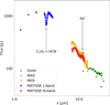 |
Fig. 1 Spectral energy distribution of X TrA. The black points represent the photometric data listed in Table A.3, and the green points correspond to IRAS data. Red and blue data points come from the current MATISSE observations, and the yellow dataset represents the MIDI observations of Paladini et al. (2017). The black arrows mark some of the spectral features we are interested in. |
3 Image reconstruction
The datasets obtained from the observations were merged before the image reconstruction process for two reasons. For one, the observations were performed over a period shorter than the star’s variability period (95 days, corresponding to ~20% of the total period of 500 days). Since available photometric data do not show very strong variations (around 0.5 amplitude variability in Johnson V magnitude; see Fig. 2) and since the MATISSE observations are in the near- to mid-infrared, the expected variability is even lower (see e.g. Le Bertre 1993). The Fourier transform of the sky brightness distribution is sampled in the (u, v)-plane, where each point corresponds to a telescope baseline and its measured spatial frequency. Combining different observations increases the (u, v)-coverage by adding more spatial frequency measurements, improving the filling of gaps done by image reconstruction techniques and reducing artefacts. The reconstruction process was carried out with the Multi-aperture Image Reconstruction Algorithm (MiRA; Thiébaut 2008), an adaptive gradient-based method, across the different wavelength windows listed in Sect. 2 via PYRA (Python for MiRA)2 and MYTHRA (Mean Astrophysical Images with PYRA3, two newly developed Python-based tools that interface with MiRA (Drevon et al., in prep.).
MiRA requires a starting image and/or model and offers a few different types of regularisation functions. For the purpose of this study, the reconstruction setup consists of a Dirac distribution as the starting image, 500 iterations and two regularisation functions, quadratic compactness and edge-preserving smoothness. The reconstruction algorithm SQUEEZE (Baron et al. 2010) was also used as an additional check of the results; additional image reconstruction efforts are discussed in Appendices D and E.
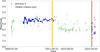 |
Fig. 2 AAVSO (Kloppenborg 2025) light curve of X TrA (blue and green symbols), from 5 February 2000 to 13 February 2025. The MIDI and MATISSE epochs of observation are highlighted in orange and red, respectively. |
4 Results
The images obtained following the reconstruction process are shown in Figs. 3 and 4. The continuum contribution was not subtracted from any of the images, as there is no near-continuum bandpass available in our data. Radial profiles were also calculated for four 90°-wide sectors, as a means of quantifying any potential asymmetries in the intensity maps. The background noise in each image was taken as the standard deviation of the pixels located within an annulus spanning 70–90% of the image’s radius, measured from the centre to the outer edge. Signal-to-noise ratio (S/N) contours are overplotted in the images, starting with a 5σ level (in magenta).
From the L band MiRA results several photospheric and circumstellar layers of X TrA can be seen. Starting with the pseudo-continuum image at 3.5 μm (middle column in Fig. 3), a region with minimal contributions from C2H2 and HCN, the star is at its smallest, with a radius of ~2 au. The photospheric diameter computed by Paladini et al. (2017) is marked by the inner dashed circle in Figs. 3 and 4, so clearly the angular extent of X TrA in the pseudo-continuum region coincides well with this. The other thing visible in this wavelength window is a horseshoe-like intensity peak in the central region, marked by a red contour in the top row of Fig. 3.
Moving outwards, the C2H2 layer at 3.8 μm (right column in Fig. 3) starts to show a more complex structure, being patchier. Of note is a south-westerly intensity peak (marked by the blue cross in the images from the top row of Fig. 3) that seems to be part of a SW-NE elongated feature and almost a complete lack of emission outside the extent of the photosphere. The peak here is cospatial with parts of the horseshoe shape seen at 3.5 μm, indicated by a higher intensity radial profile in the 180°–270° sector in both cases, suggesting that the molecular layer probed here is inhomogeneous/clumpy. Farther away from the star, the C2H2 layer is quite tenuous (has a low opacity), showing a very small amount of emission outside the photosphere in the 270°–360° and 0°–90° sectors (see the bottom-right radial profiles in Fig. 3c). One or two protrusions (towards the E–SE and one towards the west) can be seen in the S/N contours, but these cannot necessarily be considered real as they are smaller than the beam size.
The C2H2 + HCN molecular band is probed at 3.1 μm and the circumstellar envelope reaches its greatest angular size here (left column in Fig. 3), with a diameter of ~20 mas. The intensity map shows a horizontally elongated feature inside the photospheric region (along the E-W direction). Numerous features/protrusions are visible in most directions beyond the photosphere, up to radii of 10 mas (e.g. radial profile in the 270°–360° sector), and are characterised by a smooth, diffuse morphology. In combination with the high intensity of the central region, it is likely that this layer is not very optically thick due to a low column density.
The MIDI and MATISSE observations sample similar epochs, as seen in Fig. 2. A comparison between the imaging results presented here and the MIDI studies of Rau et al. (2017) and Paladini et al. (2017) finds the angular size estimates to be in good agreement. The MATISSE images at 3.5 μm give a diameter of 12 mas, while Paladini et al. (2017) estimate it to be 11 mas (based on the V-K relation of van Belle et al. 1999) and Rau et al. (2017) calculate it to be 9.8 mas (based on the V-K relation of van Belle et al. 2013). The reconstruction at 8.5 μm gives a diameter of about 19 mas, while Rau et al. (2017) compute a diameter of 21.9 ± 2.5 mas at 8 μm. The latter study mentions not finding any well-fitting models for the SiC signature seen in the visibility data, while Paladini et al. (2017) state that the visibility data indicate SiC detection around 4 stellar radii. None of the images in the L and N bands show any significant features indicative of companion presence such as disks, spirals, arcs, and tails (with typical sizes of the order of tens to a few hundred au and even up to a few thousand au; Mayer et al. 2015; Kervella et al. 2016; Decin et al. 2020).
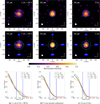 |
Fig. 3 MiRA image reconstructions for the MATISSE L band for the 3.1 μm wavelength region (leftmost column), the 3.5 μm interval (middle), and the reconstructed data for the 3.8 μm region (right). In the top row, magenta (cyan) contours indicate where the signal is 5 times (30 times) above the estimated background noise, and the inner red contour encapsulates the regions where the S/N is in the top 10% of all values across the image. The blue cross indicates the position of the emission peak seen at 3.8 μm. In the middle row, the innermost dashed cyan circle represents the photospheric diameter of Paladini et al. (2017, see our Sect. 2), while the outer circle corresponds to the photospheric diameter scaled to 12 μm, based on the size ratio of the 2 and 12 μm mass-losing dynamic models in Paladini et al. (2009). Both are marked with a dashed blue line in the radial profile plots. The sectors marked by the dotted white lines show the regions used in the plotting of the radial profiles presented in the bottom row. The images were normalised with respect to the highest intensity pixel and re-centred by computing the local average intensity using a square kernel corresponding to 3 mas in radius. The white ellipse shows the estimated beam size and its inclination at each wavelength interval. |
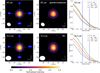 |
Fig. 4 MiRA image reconstructions for the MATISSE N band for the 8.5 (top row) and 11.3 μm (bottom row) wavelength region. Magenta (cyan) contours indicate where the signal is 5 times (30 times) the estimated background noise, and the inner red contour encapsulates the regions where the S/N is in the top 10% of all values across the image. The innermost dashed cyan circle represents the photospheric diameter from Paladini et al. (2017, see our Sect. 2), while the outer circle corresponds to the photospheric diameter scaled to 12 μm, based on the size ratio of the 2 and 12 μm mass-losing dynamic models in Paladini et al. (2009). Both are marked with a dashed blue line in the radial profile plots. The sectors marked by the dotted white lines are the regions used in the plotting of the radial profiles presented in the bottom row. The images were normalised with respect to the highest intensity pixel and re-centred on the maximum local average intensity, computed using a square kernel with a radius of 3 mas. The white ellipse shows the estimated beam size and its inclination at each wavelength interval. |
5 Discussion
5.1 Morphology
The reconstructed L band images reveal an asymmetric structure in the molecular layers, with elongations and protrusions especially visible in the C2H2 + HCN layer. This result is not unexpected, as Hulberg et al. (2025) and Drevon et al. (2022) attribute the nature of the spectrum and morphology of the images to the molecular influence of C2H2 and C2H2 + HCN, the latter study exhibiting similar morphological features in the image of R Scl at 3.1 μm (i.e. elongated features and asymmetric protrusions).
It has previously been found that the intensity of the spectral features of molecules such as C2H2 in the L and N bands are correlated with stellar pulsation phase (Loidl et al. 2000; Ohnaka et al. 2007). This would translate to changes in size when looking at the corresponding specific wavelengths. Other more recent studies of carbon stars (Drevon et al. 2022; Planquart et al. 2024; Hulberg et al. 2025, all done with MATISSE) find similar angular sizes and a similar wavelength dependence regarding the scale of the emission as presented here, namely that the extent of the source is at its largest in the 3.1 μm region and in the N band and at its smallest in the L band pseudo-continuum at 3.5 μm. Table 1 shows a comparison between stellar parameters for three different carbon stars that have been imaged with MATISSE and the ratio of their size in the 3.1 micron C2H2 + HCN feature and the L band pseudo-continuum at 3.5 micron (θ3.1/3.5). When observed at different pulsation phases, the ratios follow the expected behaviour of being larger close to maximum light (Woodruff et al. 2008). Since X TrA’s irregular aspect makes it difficult to determine the pulsation phase, this comparison between the θ3.1/3.5 values suggests X TrA could have been close to maximum light at the time of MATISSE observations.
Carbon stars recently imaged with MATISSE.
5.2 Clumpiness
Closer inspection of the 3.1 and 3.8 μm layers indicates that the molecular distribution is inhomogeneous, pointing to clumpy structures within the circumstellar environment. The 3D models of dust-driven winds in AGB stars by Freytag & Höfner (2023) support the idea that an inhomogeneous gas distribution due to convection and pulsation results in anisotropic and clumpy dust formation. Although these models are based on an oxygen-rich chemistry, the mechanisms of structure formation in the circumstellar environment are independent of the C/O ratio and also apply to carbon stars. Similarly, Velilla-Prieto et al. (2023) detect HCN emission in the close vicinity of IRC+10°216, with a morphology reminiscent of larger-scale structures previously identified in its extended circumstellar environment, reaching the same conclusion that localised conditions can drive clumpy outflows. All this suggests that the C2H2 + HCN feature might typically appear as a clumpy layer around the target object, and the resulting dust structures may exhibit similar morphologies.
The stark difference between the C2H2 + HCN and C2H2 emission beyond the extent of the photosphere is also of interest. The difference could arise because the C2H2 band at 3.1 μm is significantly stronger than that at 3.8 μm, but HCN could also contribute. The latter molecule is believed to form in the inner wind of AGB stars (within a few stellar radii, Cherchneff 2012), and the observed emission difference outside the photosphere may provide some initial constraints on the HCN column density in the close environment of X TrA. Detailed chemical modelling of the wind would therefore be required to quantify the significance of the HCN contribution.
5.3 Dust layer
Due to the spatial resolution of the instrument in the N band (8–13 mas), data only probe the first lobe of the visibility curve without entirely resolving the central source (see Fig. C.2). Nevertheless, even here the intensity map takes a slightly elliptical shape with an elongated central peak (Fig. 4), although in the north-south direction, and the SiC band at 11.3 μm (bottom row in Fig. 4) shows a higher intensity towards the south-west (more clearly shown by the 180°–270° sector in the rightmost plot on the bottom row of Fig. 4). The reconstructed source has a diameter of 19 mas (3.5 au) in the N band, similar to the C2H2 + HCN layer, increasing ever so slightly at 11.3 μm and corresponding to the inferred diameter at 12 μm from the relation of Paladini et al. (2009, represented by the outer dashed cyan line in the images). No significant emission is seen outside the circumstellar dust disk.
The MATISSE images at 11.3 μm do not show any significant features at this range, just as the ones at 8.5 μm. The dust thermal emission at 8.5 μm is mostly caused by amorphous carbon and, just as SiC, is expected to form close to the star. It is therefore likely that the N band images show no significant difference due to a similar spatial distribution of the two species.
6 Conclusions
In this paper we have presented the first MATISSE images of the irregular variable X TrA. Image reconstruction with MiRA reveals an angular diameter range of 10 to 20 mas (corresponding to a radius of 2–3.5 au), with the smallest size in the 3.5 μm pseudo-continuum band and the largest in the C2H2 + HCN molecular and dust emission bands, at 3.1 and 11.3 μm, respectively. The reconstructed images confirm previous photospheric diameter estimates of Paladini et al. (2017) and Rau et al. (2017) and show some interesting features, such as elongations and some asymmetric protrusions. They are likely caused by convection and pulsation effects, which can result in inhomogeneous gas distributions and subsequently anisotropic and/or clumpy dust formation (Freytag & Höfner 2023). No significant signs of a companion’s effects are detected in the image data, down to the 5σ level. The angular sizes estimated here, and their wavelength dependence, follow similar values and trends as presented in other recent studies of carbon stars (Drevon et al. 2022; Planquart et al. 2024; Hulberg et al. 2025). The highly asymmetric appearance of the C2H2 + HCN layer is not the first case of a carbon-rich star showing a complex morphology in the close stellar environment (Drevon et al. 2022; Velilla-Prieto et al. 2023), indicating that the C2H2 + HCN molecular spatial distribution is clumpy in nature. The angular resolution of the N band data was unsatisfactory, likely due to the calibrators being too faint in this wavelength range and the baselines too short. Therefore, the images do not show any distinct features within the circumstellar dust disk, suggesting that any SiC present is likely co-spatial with amorphous carbon and, therefore, making the two difficult to distinguish. Additional image data, combined with chemical modelling efforts, could help disentangle the role of HCN in the apparent difference between the C2H2 + HCN and C2H2 layers. In the N band, using the 202m baseline offered by the extended Auxiliary Telescope configuration would theoretically increase the angular resolution by ~35%, potentially enabling a better constraint to be placed on the size of any circumstellar features.
Acknowledgements
The research leading to these results has received funding from the European Union’s Horizon 2020 research and innovation programme under Grant Agreement 101004719 (ORP). V.R. acknowledges the support from the ESO Early-Career Scientific Visitor Programme. K.O. acknowledges the support of the Agencia Nacional de Investigación Científica y Desarrollo (ANID) through the FONDECYT Regular grant 1240301. J.S.-B. acknowledges the support received by the UNAM DGAPA-PAPIIT project AG101025. The work of J.A.H. and C.S.C. is part of the I+D+i project PID2023-146056NB-C22 funded by Spanish MCIN/AEI/10.13039/501100011033. L.V-P. acknowledges Spanish Ministerio de Ciencia, Innovación y Universidades for funding support through project PID2020-117034RJ-I00, PID2023-147545NB-I00 and grant RYC2023-045648-I. S.H. acknowledges funding from the European Research Council (ERC) under the European Union’s Horizon 2020 research and innovation programme (Grant agreement No. 883867, project EXWINGS) and the Swedish Research Council (Vetenskapsrådet, grant number 2019-04059). J.P.F. acknowledges funding support from Spanish Ministerio de Ciencia, Innovación, y Universidades through grants PID2023-147545NB-I00, PID2023-146056NB-C21, and PID2023-146056NB-C22.
References
- Abia, C., de Laverny, P., Romero-Gómez, M., & Figueras, F. 2022, A&A, 664, A45 [NASA ADS] [CrossRef] [EDP Sciences] [Google Scholar]
- Andriantsaralaza, M., Ramstedt, S., Vlemmings, W. H. T., et al. 2021, A&A, 653, A53 [NASA ADS] [CrossRef] [EDP Sciences] [Google Scholar]
- Andriantsaralaza, M., Ramstedt, S., Vlemmings, W. H. T., & De Beck, E. 2022, A&A, 667, A74 [NASA ADS] [CrossRef] [EDP Sciences] [Google Scholar]
- Baron, F., Monnier, J. D., & Kloppenborg, B. 2010, SPIE Conf. Ser., 7734, 77342I [Google Scholar]
- Bergeat, J., & Chevallier, L. 2005, A&A, 429, 235 [NASA ADS] [CrossRef] [EDP Sciences] [Google Scholar]
- Bourgés, L., Lafrasse, S., Mella, G., et al. 2014, ASP Conf. Ser., 485, 223 [NASA ADS] [Google Scholar]
- Cherchneff, I. 2012, A&A, 545, A12 [NASA ADS] [CrossRef] [EDP Sciences] [Google Scholar]
- Cox, N. L. J., Kerschbaum, F., van Marle, A. J., et al. 2012, A&A, 537, A35 [NASA ADS] [CrossRef] [EDP Sciences] [Google Scholar]
- Cruzalèbes, P., Petrov, R. G., Robbe-Dubois, S., et al. 2019, MNRAS, 490, 3158 [Google Scholar]
- De Beck, E., Decin, L., de Koter, A., et al. 2010, A&A, 523, A18 [NASA ADS] [CrossRef] [EDP Sciences] [Google Scholar]
- Decin, L., Montargès, M., Richards, A. M. S., et al. 2020, Science, 369, 1497 [Google Scholar]
- Doan, L., Ramstedt, S., Vlemmings, W. H. T., et al. 2020, A&A, 633, A13 [NASA ADS] [CrossRef] [EDP Sciences] [Google Scholar]
- Drevon, J., Millour, F., Cruzalèbes, P., et al. 2022, A&A, 665, A32 [NASA ADS] [CrossRef] [EDP Sciences] [Google Scholar]
- Drevon, J., Millour, F., Cruzalèbes, P., et al. 2024, MNRAS, 527, L88 [Google Scholar]
- Duvert, G., Young, J., & Hummel, C. A. 2017, A&A, 597, A8 [NASA ADS] [CrossRef] [EDP Sciences] [Google Scholar]
- Eggleton, P. P., & Tokovinin, A. A. 2008, MNRAS, 389, 869 [Google Scholar]
- Freytag, B., & Höfner, S. 2023, A&A, 669, A155 [NASA ADS] [CrossRef] [EDP Sciences] [Google Scholar]
- Gail, H.-P., & Sedlmayr, E. 2013, Physics and Chemistry of Circumstellar Dust Shells (Cambridge: Cambridge University Press) [Google Scholar]
- Herwig, F. 2005, ARA&A, 43, 435 [Google Scholar]
- Höfner, S., & Olofsson, H. 2018, A&A Rev., 26, 1 [CrossRef] [Google Scholar]
- Hron, J., Loidl, R., Hoefner, S., et al. 1998, A&A, 335, L69 [NASA ADS] [Google Scholar]
- Hulberg, J., Rau, G., & Wittkowski, M. 2025, ApJ, 982, 135 [Google Scholar]
- Izumiura, H., Kester, D. J. M., de Jong, T., et al. 1995, Ap&SS, 224, 495 [Google Scholar]
- Jørgensen, U. G., Hron, J., & Loidl, R. 2000, A&A, 356, 253 [NASA ADS] [Google Scholar]
- Kerschbaum, F., Maercker, M., Brunner, M., et al. 2017, A&A, 605, A116 [NASA ADS] [CrossRef] [EDP Sciences] [Google Scholar]
- Kervella, P., Homan, W., Richards, A. M. S., et al. 2016, A&A, 596, A92 [NASA ADS] [CrossRef] [EDP Sciences] [Google Scholar]
- Kipper, T. 2004, Balt. Astron., 13, 573 [NASA ADS] [Google Scholar]
- Kloppenborg, B. K. 2025, Observations from the AAVSO International Database [Google Scholar]
- Knapp, G. R., Jorissen, A., & Young, K. 1997, A&A, 326, 318 [NASA ADS] [Google Scholar]
- Le Bertre, T. 1993, A&AS, 97, 729 [NASA ADS] [Google Scholar]
- Loidl, R., Hron, J., Jorgensen, U. G., & Höfner, S. 2000, in ESA Special Publication, Vol. 456, ISO Beyond the Peaks: The 2nd ISO Workshop on Analytical Spectroscopy, eds. A. Salama, M. F. Kessler, K. Leech, & B. Schulz, 315 [Google Scholar]
- Lopez, B., Lagarde, S., Petrov, R. G., et al. 2022, A&A, 659, A192 [NASA ADS] [CrossRef] [EDP Sciences] [Google Scholar]
- Mayer, A., Jorissen, A., Kerschbaum, F., et al. 2015, ASP Conf. Ser., 497, 181 [Google Scholar]
- Montargès, M., Malfait, J., Esseldeurs, M., et al. 2025, A&A, 699, A22 [NASA ADS] [CrossRef] [EDP Sciences] [Google Scholar]
- Ohnaka, K., Driebe, T., Weigelt, G., & Wittkowski, M. 2007, A&A, 466, 1099 [NASA ADS] [CrossRef] [EDP Sciences] [Google Scholar]
- Paladini, C., Aringer, B., Hron, J., et al. 2009, A&A, 501, 1073 [NASA ADS] [CrossRef] [EDP Sciences] [Google Scholar]
- Paladini, C., Klotz, D., Sacuto, S., et al. 2017, A&A, 600, A136 [NASA ADS] [CrossRef] [EDP Sciences] [Google Scholar]
- Paladini, C., Baron, F., Jorissen, A., et al. 2018, Nature, 553, 310 [NASA ADS] [CrossRef] [Google Scholar]
- Percy, J. R., Esteves, S., Lin, A., Menezes, C., & Wu, S. 2009, jaavso, 37, 71 [Google Scholar]
- Pitman, K. M., Hofmeister, A. M., Corman, A. B., & Speck, A. K. 2008, A&A, 483, 661 [NASA ADS] [CrossRef] [EDP Sciences] [Google Scholar]
- Planquart, L., Paladini, C., Jorissen, A., et al. 2024, A&A, 687, A306 [NASA ADS] [CrossRef] [EDP Sciences] [Google Scholar]
- Ramstedt, S., Mohamed, S., Vlemmings, W. H. T., et al. 2017, A&A, 605, A126 [NASA ADS] [CrossRef] [EDP Sciences] [Google Scholar]
- Rau, G., Hron, J., Paladini, C., et al. 2017, A&A, 600, A92 [NASA ADS] [CrossRef] [EDP Sciences] [Google Scholar]
- Rosales-Guzmán, A., Sanchez-Bermudez, J., Paladini, C., et al. 2023, A&A, 674, A62 [NASA ADS] [CrossRef] [EDP Sciences] [Google Scholar]
- Schneider, R., Valiante, R., Ventura, P., et al. 2014, MNRAS, 442, 1440 [NASA ADS] [CrossRef] [Google Scholar]
- Schöier, F. L. & Olofsson, H. 2001, A&A, 368, 969 [NASA ADS] [CrossRef] [EDP Sciences] [Google Scholar]
- Sloan, G. C., Little-Marenin, I. R., & Price, S. D. 1998, AJ, 115, 809 [NASA ADS] [CrossRef] [Google Scholar]
- Thiébaut, E. 2008, SPIE Conf. Ser., 7013, 70131I [Google Scholar]
- Thiébaut, É., & Young, J. 2017, J. Opt. Soc. Am. A, 34, 904 [Google Scholar]
- van Belle, G. T., Lane, B. F., Thompson, R. R., et al. 1999, AJ, 117, 521 [NASA ADS] [CrossRef] [Google Scholar]
- van Belle, G. T., Paladini, C., Aringer, B., Hron, J., & Ciardi, D. 2013, ApJ, 775, 45 [NASA ADS] [CrossRef] [Google Scholar]
- Velilla-Prieto, L., Fonfría, J. P., Agúndez, M., et al. 2023, Nature, 617, 696 [NASA ADS] [CrossRef] [Google Scholar]
- Vlemmings, W., Khouri, T., O’Gorman, E., et al. 2017, Nat. Astron., 1, 848 [NASA ADS] [CrossRef] [Google Scholar]
- Vlemmings, W., Khouri, T., Bojnordi Arbab, B., De Beck, E., & Maercker, M. 2024, Nature, 633, 323 [Google Scholar]
- Wallerstein, G., & Knapp, G. R. 1998, ARA&A, 36, 369 [Google Scholar]
- Woodruff, H. C., Tuthill, P. G., Monnier, J. D., et al. 2008, ApJ, 673, 418 [NASA ADS] [CrossRef] [Google Scholar]
Available at https://gitlab.oca.eu/MATISSE/tools
Available at https://amhra.oca.eu/AMHRA/oifits-modeler/input.htm
Appendix A Observational details
Calibrator details.
Observation log for target X TrA.
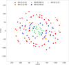 |
Fig. A.1 VLTI/MATISSE uv coverage of X TrA, colour-coded according to the telescope configuration used. |
Appendix B Input MATISSE data visualised
Here we present the interferometric data of X TrA that were used to obtain the images presented in this study. The figures shown here present L band squared-visibility curves (Fig. B.1a), N band visibility amplitudes (Fig. B.1b) and their corresponding closure phase data (Fig. B.1c and B.1d).
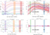 |
Fig. B.1 Squared visibilities, visibility amplitudes, and closure phases of the input MATISSE data used in the image reconstruction process, colour-coded according to telescope configuration. The shaded areas represent the wavelength regions selected for image reconstruction (described in Sect. 2), except for the grey area shown in the N band plots. This marks a region of strong ozone absorption that falls in the wavelength range covered by the MATISSE instrument. The shaded areas without a label correspond to the selected pseudo-continuum bands. |
Appendix C Additional MiRA reconstruction results
The images shown in the article are obtained via the quadratic compactness regularisation function of MiRA, as the edge-preserving smoothness function produced unrealistic results in many cases (e.g. gaps in the centre, spots with nothing in-between). The figures presented in this section show the observed data versus the MiRA reconstructed observables, corresponding to each of the wavelength channels used in the article.
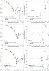 |
Fig. C.1 Squared visibilities (left) and closure phases (right) of the reconstructed images (blue dots) compared to the input MATISSE data (orange dots). |
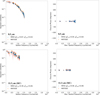 |
Fig. C.2 Squared visibilities (left) and closure phases (right) of the reconstructed images (blue dots) compared to the input MATISSE data (orange dots). |
Appendix D SQUEEZE results
As opposed to MiRA, SQUEEZE fits the interferometric data via a Markov chain Monte Carlo algorithm. The total-variation regularisation function was used, this reconstruction method being suitable for cases where one is interested in keeping prominent features, as it handles well uniform areas that show steep (but localised) changes. Similar to the edge-preserving smoothness regularisation of MiRA, this method produces imprecise artefacts, while MiRA’s quadratic compactness gives rise to artefacts in the shape of ripples around structures (Thiébaut & Young 2017). The same parameters used for the MiRA reconstruction (pixel size and field-of-view) are used to reconstruct an image with Squeeze, with the final image representing the median of ten chains. This serves as an additional verification of the images. If the two algorithms converge on a similar solution, then the result can be considered reliable.
As seen in Fig. D.1, the overall size of the object is the same as in the MiRA images. The more prominent features are also reproduced, such as the east-west elongation seen at 3.1 μm (although here it is part of a larger structure that also extends towards the north) and the south-westerly peak at 3.5 and 3.8 μm. In the case of SQUEEZE, the emission peak seen at 3.8 μm seems to also overlap with the one at 3.1 μm. The numerous small structures outside the stellar disk that reach the 5σ level in the pseudo-continuum band are most likely artefacts resulting from the median averaging of the images. Combined with the background noise being much lower than in MiRA reconstructions, this could enhance the prominence of spurious background features.
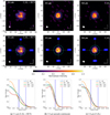 |
Fig. D.1 SQUEEZE reconstructed images for the L band data. See Fig. 3 for a full description of the contours, labels, and markers. |
Appendix E Rotation tests
To assess the reliability of some features in the reconstructed images, rotation tests were used, following the approach of Planquart et al. (2024). This was done with the OIFits modeler software4 (Duvert et al. 2017), which creates synthetic data from the input uv-coverage and the assumed image. In this case, the uncertainties of the observational data are used, as error bars are not provided for the synthetic observables by OIFits modeler. The synthetic data are manipulated in a way that produces a rotated image upon a subsequent reconstruction attempt. When comparing the initial reconstruction with the rotated one, features that are present in both cases can be deemed as genuine, while the ones that disappear are most likely artefacts of the reconstruction process and can therefore not be trusted.
As seen in Figs. E.1 and E.2, the data were rotated by 90° anti-clockwise and most of the major features and peaks in intensity are recovered quite well. The 3.1 and 3.8 μm images shows some differences, specifically in intensity. The major features such as the protrusions and the elongation in the middle are still there, but the intensity is spread out more evenly across the entire surface of this layer. In the case of the 3.1 μm image, the intensity drop is quite significant, and some larger artefacts are visible towards the edges. This is most likely a product of the reconstruction algorithm, as the chosen regularisation function (quadratic compactness) can smooth out some of the finer details and sometimes can even lead to overly smoothed images.
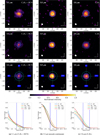 |
Fig. E.1 MiRA original image reconstructions (top row) versus MiRA reconstruction of the OIFits modeler data, i.e. MiRA images rotated 90° anti-clockwise (rows 2–4), for the MATISSE L band. See Fig. 3 for a full description of the contours, labels, and markers. |
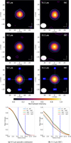 |
Fig. E.2 MiRA original image reconstructions (top row) versus MiRA reconstruction of the OIFits modeler data, i.e. MiRA images rotated 90° anti-clockwise (rows 2–4), for the MATISSE N band. See Fig. 4 for a full description of the contours, labels, and markers. |
All Tables
All Figures
|
Fig. 1 Spectral energy distribution of X TrA. The black points represent the photometric data listed in Table A.3, and the green points correspond to IRAS data. Red and blue data points come from the current MATISSE observations, and the yellow dataset represents the MIDI observations of Paladini et al. (2017). The black arrows mark some of the spectral features we are interested in. |
| In the text | |
|
Fig. 2 AAVSO (Kloppenborg 2025) light curve of X TrA (blue and green symbols), from 5 February 2000 to 13 February 2025. The MIDI and MATISSE epochs of observation are highlighted in orange and red, respectively. |
| In the text | |
|
Fig. 3 MiRA image reconstructions for the MATISSE L band for the 3.1 μm wavelength region (leftmost column), the 3.5 μm interval (middle), and the reconstructed data for the 3.8 μm region (right). In the top row, magenta (cyan) contours indicate where the signal is 5 times (30 times) above the estimated background noise, and the inner red contour encapsulates the regions where the S/N is in the top 10% of all values across the image. The blue cross indicates the position of the emission peak seen at 3.8 μm. In the middle row, the innermost dashed cyan circle represents the photospheric diameter of Paladini et al. (2017, see our Sect. 2), while the outer circle corresponds to the photospheric diameter scaled to 12 μm, based on the size ratio of the 2 and 12 μm mass-losing dynamic models in Paladini et al. (2009). Both are marked with a dashed blue line in the radial profile plots. The sectors marked by the dotted white lines show the regions used in the plotting of the radial profiles presented in the bottom row. The images were normalised with respect to the highest intensity pixel and re-centred by computing the local average intensity using a square kernel corresponding to 3 mas in radius. The white ellipse shows the estimated beam size and its inclination at each wavelength interval. |
| In the text | |
|
Fig. 4 MiRA image reconstructions for the MATISSE N band for the 8.5 (top row) and 11.3 μm (bottom row) wavelength region. Magenta (cyan) contours indicate where the signal is 5 times (30 times) the estimated background noise, and the inner red contour encapsulates the regions where the S/N is in the top 10% of all values across the image. The innermost dashed cyan circle represents the photospheric diameter from Paladini et al. (2017, see our Sect. 2), while the outer circle corresponds to the photospheric diameter scaled to 12 μm, based on the size ratio of the 2 and 12 μm mass-losing dynamic models in Paladini et al. (2009). Both are marked with a dashed blue line in the radial profile plots. The sectors marked by the dotted white lines are the regions used in the plotting of the radial profiles presented in the bottom row. The images were normalised with respect to the highest intensity pixel and re-centred on the maximum local average intensity, computed using a square kernel with a radius of 3 mas. The white ellipse shows the estimated beam size and its inclination at each wavelength interval. |
| In the text | |
|
Fig. A.1 VLTI/MATISSE uv coverage of X TrA, colour-coded according to the telescope configuration used. |
| In the text | |
|
Fig. B.1 Squared visibilities, visibility amplitudes, and closure phases of the input MATISSE data used in the image reconstruction process, colour-coded according to telescope configuration. The shaded areas represent the wavelength regions selected for image reconstruction (described in Sect. 2), except for the grey area shown in the N band plots. This marks a region of strong ozone absorption that falls in the wavelength range covered by the MATISSE instrument. The shaded areas without a label correspond to the selected pseudo-continuum bands. |
| In the text | |
|
Fig. C.1 Squared visibilities (left) and closure phases (right) of the reconstructed images (blue dots) compared to the input MATISSE data (orange dots). |
| In the text | |
|
Fig. C.2 Squared visibilities (left) and closure phases (right) of the reconstructed images (blue dots) compared to the input MATISSE data (orange dots). |
| In the text | |
|
Fig. D.1 SQUEEZE reconstructed images for the L band data. See Fig. 3 for a full description of the contours, labels, and markers. |
| In the text | |
|
Fig. E.1 MiRA original image reconstructions (top row) versus MiRA reconstruction of the OIFits modeler data, i.e. MiRA images rotated 90° anti-clockwise (rows 2–4), for the MATISSE L band. See Fig. 3 for a full description of the contours, labels, and markers. |
| In the text | |
|
Fig. E.2 MiRA original image reconstructions (top row) versus MiRA reconstruction of the OIFits modeler data, i.e. MiRA images rotated 90° anti-clockwise (rows 2–4), for the MATISSE N band. See Fig. 4 for a full description of the contours, labels, and markers. |
| In the text | |
Current usage metrics show cumulative count of Article Views (full-text article views including HTML views, PDF and ePub downloads, according to the available data) and Abstracts Views on Vision4Press platform.
Data correspond to usage on the plateform after 2015. The current usage metrics is available 48-96 hours after online publication and is updated daily on week days.
Initial download of the metrics may take a while.