| Issue |
A&A
Volume 705, January 2026
|
|
|---|---|---|
| Article Number | L8 | |
| Number of page(s) | 9 | |
| Section | Letters to the Editor | |
| DOI | https://doi.org/10.1051/0004-6361/202557621 | |
| Published online | 09 January 2026 | |
Letter to the Editor
Connections between the cycle-to-cycle light curve and O−C variations of the Blazhko RR Lyrae stars
Konkoly Observatory, HUN-REN Research Centre for Astronomy and Earth Sciences, MTA Centre of Excellence Konkoly Thege u. 15-17. 1121 Budapest, Hungary
★ Corresponding author: This email address is being protected from spambots. You need JavaScript enabled to view it.
Received:
9
October
2025
Accepted:
3
December
2025
Abstract
Context. Recent studies have shown that the irregular O−C variations observed in many non-Blazhko RR Lyrae stars may result from random, cycle-to-cycle (C2C) variations in their light curves. However, centuries-long data series reveal that the O−C diagrams of Blazhko stars exhibit particularly large-amplitude, irregular variations.
Aims. In this letter, we extend the previous investigation of non-Blazhko stars to Kepler Blazhko stars to explore the role of C2C variations in the O−C diagrams.
Methods. We derived the O−C diagrams from Kepler space telescope light curves using a precise template-fitting method. Based on their Fourier analyses, we also constructed residual O−C diagrams that were pre-whitened for frequencies associated with the Blazhko effect. We then fitted the same statistical models to both types of O−Cs that we had previously applied to non-Blazhko stars.
Results. The optimal statistical model includes the C2C variation for 74% of the O−C curves in our Blazhko sample, and the parameter describing the strength of the C2C variation is significantly larger than that obtained for non-Blazhko stars. This may explain the strong irregular O−C variations previously observed in Blazhko stars. Furthermore, we found a strong positive correlation between the C2C variation strength and the amplitude of the frequency-modulation component of the Blazhko effect, indicating a connection between the two phenomena.
Key words: methods: data analysis / techniques: photometric / stars: oscillations / stars: variables: RR Lyrae
© The Authors 2026
 Open Access article, published by EDP Sciences, under the terms of the Creative Commons Attribution License (https://creativecommons.org/licenses/by/4.0), which permits unrestricted use, distribution, and reproduction in any medium, provided the original work is properly cited.
This article is published in open access under the Subscribe to Open model. This email address is being protected from spambots. You need JavaScript enabled to view it. to support open access publication.
1. Introduction
RR Lyrae stars are horizontal-branch stars located within the classical instability strip of the Hertzsprung–Russell diagram. They pulsate radially in the fundamental mode (RRab), first-overtone mode (RRc), or both modes (RRd) (see e.g. Catelan 2009). In addition to the brightness variations caused by radial pulsation, the light curves of many RR Lyrae stars display simultaneous amplitude (AM) and frequency (FM) modulations with periods much longer than the pulsation period, ranging from several days to several years (see Jurcsik & Smitola 2016; Netzel et al. 2018; Skarka et al. 2020). This phenomenon is known as the Blazhko effect (for detailed reviews, see e.g. Smolec 2016 and Kovács 2016).
Numerous studies have investigated the long-term period variation of RR Lyrae stars using O−C diagrams (e.g. Le Borgne et al. 2007; Szeidl et al. 2011; Jurcsik et al. 2012; Prudil et al. 2019; Hajdu et al. 2021). The analyses of these works have revealed that some RR Lyrae stars exhibit slow, regular period changes consistent with stellar evolutionary models, whereas other RR Lyrae stars show much faster irregular variations. Although this latter group includes several RRab and RRc stars that do not show the Blazhko effect, Blazhko stars are always found among them. Their irregular O−C variations generally exhibit higher amplitudes than those of non-Blazhko stars. In other words, it seems that the Blazhko effect gives rise to irregular O−C variations. However, it remains unclear how this occurs and why the amplitudes of irregular O−C variations are larger in Blazhko than in non-Blazhko stars.
Benkő et al. (2025) recently demonstrated that the vast majority of irregular O−C diagrams of non-Blazhko RR Lyrae stars observed by the Kepler and TESS space telescopes can be explained by random cycle-to-cycle (C2C) variations in their light curves. In this letter, we extend that analysis to Blazhko stars in order to examine whether similar variations can account for their O−C behaviour as well.
2. Data and methods
Since the characteristic period of the Blazhko effect is typically much longer than the pulsation period, we used the four-year Kepler dataset (Borucki et al. 2010), which provides uninterrupted high-precision space photometry suitable for detailed C2C analysis. Benkő et al. (2014) investigated the Blazhko RR Lyrae stars observed by the Kepler space telescope, and in this study we used the corrected (tailor-made) light curves provided by them. We used 15 Blazhko RRab stars from Benkő et al. (2014). The work of Forró et al. (2022), who identified ten Blazhko RR Lyrae stars in the background pixels of the original Kepler field, proved useful in compiling a larger homogeneous sample observed with the same instrument, cadence, and photometric setup. We performed O−C analyses for all the RR Lyrae stars found by Forró et al. (2022); two of them appear to be new Blazhko candidates. Thus, our final sample consists of 27 RR Lyrae (25 RRab and 2 RRc) stars. Table A.2 lists the stars included in this study.
For consistency with previous work on non-Blazhko stars (Benkő et al. 2025), we constructed the O−C diagrams using a template-fitting method (Hertzsprung 1919). For the definition and a detailed discussion of O−C diagrams, we refer to Sterken 2005. The used template fitting method is described in more detail in Benkő et al. (2019). In brief, we derived a template from the Fourier fit of the average light curve, fitted Fourier sums with different numbers of terms to the folded light curve, and determined the optimal number of terms using the Akaike information criterion. For our sample, this number ranged from 4 to 39. The template was then shifted horizontally and scaled vertically by a unique multiplier of each pulsation cycle. The phase shift obtained from the fit was adopted as the O−C value. The resulting diagrams are shown in red in Figs. A.1.
For high-amplitude O−C diagrams, the template-fitting method and the classical polynomial fitting yielded similar results, but for low-amplitude cases, the template-fitting method revealed considerably more detail and visibly better precision. The improved accuracy of the method is illustrated by V838 Cyg, whose small-amplitude Blazhko modulation nevertheless allowed a reliable O−C curve to be derived, in contrast to Benkő et al. (2014). Benkő et al. (2014) reported an average timing uncertainty of about one minute (≈6.9 ⋅ 10−4 d). In this work, we estimated individual alignment uncertainties using Monte Carlo simulations; these are shown as light yellow error bars in Fig. A.1. Typical 1σ uncertainties of individual O−C points range from 3.4 × 10⁻⁵ − 1.7 × 10⁻³ d for the original Kepler targets and from 9 × 10⁻⁴ − 4.7 × 10⁻³ d for the background stars.
The blue curves in Fig. A.1 present the first O−C diagrams for the stars from Forró et al. (2022). In the best cases, the accuracy of these diagrams matches that of the original Kepler targets (red curves). The higher dispersion of some curves is partly due to the faintness of these background stars and, in some quarters, to partial flux loss caused by imperfect photometric masks.
The O−C diagrams were Fourier-analysed using the PERIOD04 program (Lenz & Breger 2005). The highest peak was assigned to the main Blazhko frequency. Benkő et al. (2014) found that in multi-periodic Blazhko stars, the relative strengths of the AM and FM components may differ: one period can dominate the amplitude modulation, while another dominates the frequency modulation. The Fourier spectra of the O−C curves contain only the FM component of the Blazhko effect; therefore, the Blazhko frequency referred to here as dominant actually means dominant in FM. These frequencies are listed in the fourth column of Table A.2. During the Fourier analysis of the O−C diagrams, we found that the significant frequencies correspond to the Blazhko frequencies themselves, their harmonics, sub-harmonics, and – in cases of multiple Blazhko modulations – linear combinations of those frequencies. Pre-whitening all such terms (typically one to eight per star) yielded the O−C residuals. Although the light-curve shape variations of Blazhko stars may introduce systematic phase shifts in the determination of O−Cs, any such effects occur on the Blazhko timescale and therefore appear in the O−C spectra. Consequently, the residuals remain free of these systematics. The frequencies we removed, along with their possible identifications, are given in Table A.1.
We also detected significant frequencies associated with long-term trends, the origins of which remain uncertain. They could arise from instrumental effects, very long Blazhko cycles, or additional physical processes. Alternatively, they might reflect apparent period changes caused by C2C variations, as proposed in our previous work. Because the focus of this paper is the study of such variations, we did not pre-whiten these frequencies, and therefore they remain in what we refer to as the ‘O−C residuals’. No residual curve was constructed for the two RRc stars, as their O−C variations have extremely long periods (if they are periodic at all) and cannot be clearly separated from the Blazhko or other long-term effects.
Benkő et al. (2025) analysed the O−C diagrams of Kepler non-Blazhko RR Lyrae stars using the statistical framework of Koen (2006). In this work, we adopted the same approach, assuming that the instantaneous pulsation period, Pi, can be expressed as the sum of three components:
 (1)
(1)
where ⟨P⟩ is the constant mean period, the summation term represents a general smooth period variation, ξj is assumed to be a zero-mean uncorrelated random variable, and ηi accounts for the effect of C2C variations in the light curve on the instantaneous period.
Moreover, the construction of O−C diagrams is inherently affected by timing noise (or phase noise),
 (2)
(2)
where ti is the measured time, Ti is the true time, and ei is a random variable with zero mean. The phase noise, ϕi, and timing noise, ei, are related through ϕi = 2πei/P, where P is the pulsation period. Thus, three random variables are involved, e, ξ, and η, with corresponding standard deviations, σe, σξ, and ση.
Benkő et al. (2025) investigated four statistical models based on these assumptions to determine which provided the best fit to the observational data. The four models are as follows: M1, phase noise only; M2, phase noise plus C2C variation; M3, a combination of phase noise and real period change; and M4, including all three effects simultaneously.
3. Results and discussion
3.1. New Blazhko candidates
Forró et al. (2022) identified ten Blazhko stars in the background pixels of the Kepler space telescope but did not examine their O−C diagrams. Forró et al. (2022) noted that KPP23 and KPP26 show amplitude changes, which they attributed to instrumental effects. Although the light curve of KPP23 is of relatively poor quality, its O−C diagram clearly shows variability (see Fig. A.1). The corresponding Fourier spectrum contains two significant frequencies: fB = 0.00543 ± 0.000046 d−1 (S/N = 5.99) and 2fB = 0.01086 ± 0.000046 d−1 (S/N = 12.16). The derived period, PB = 184.1 ± 1.6 d, is indeed close to twice the duration of a Kepler quarter, yet no systematic timing error of this kind is known for the Kepler space telescope. This makes KPP23 a strong candidate for a new Blazhko RR Lyrae star. In contrast, the O−C diagram for KPP26 appears to be constant (last panel in Fig. A.1), and no significant frequency can be found in its spectrum, suggesting that its reported amplitude variation is most likely instrumental in origin. KPP14 is an RRc star for which Forró et al. (2022) did not report amplitude modulation. However, its O−C diagram displays a clear, smooth variation (see Fig. A.1). If this variation is periodic, its period may be approximately ∼982 days.
3.2. Revisited O−C spectra
The Fourier content of the O−C diagrams constructed using the template-fitting method differs slightly in some cases from that reported by Benkő et al. (2014). In the case of V783 Cyg, two frequencies were detected (fs and fB − fs; see Table A.1) that were not identified by Benkő et al. (2014). The presence of a secondary Blazhko modulation may explain the non-strictly periodic behaviour of the O−C curve, which had previously been interpreted as an indication of chaotic modulation (Plachy et al. 2014).
For V355 Lyr, contrary to the findings of Benkő et al. (2014), the dominant frequency in AM is also dominant in the O−C diagram. In the case of V450 Lyr, we detected the same frequencies as Benkő et al. (2014), but with different relative amplitudes. Accordingly, we interpreted the signals as fB and its harmonic 2fB, rather than the sub-harmonic fB/2. This implies that the dominant frequencies differ between AM and FM.
In the case of V366 Lyr, similar to V355 Lyr, the dominant frequencies coincide in AM and FM, which again is in contrast to the results published by Benkő et al. (2014). The difference between the amplitudes of the two frequencies, which determines the order of the dominant and secondary effects, is 4 × 10⁻⁵ d, and it is comparable to the uncertainty of the amplitudes (σ ∼ 1.6 × 10⁻⁵ d).
3.3. Cycle-to-cycle variation on Blazhko stars
We applied the same statistical framework as in Benkő et al. (2025). We analysed both the original O−C data and the residual O−C curves from which all frequencies related to the Blazhko effect had been removed. In contrast to the non-Blazhko stars, the results for certain Blazhko stars were sensitive to the adopted limits of the parameters σmin and σmax; different bounds often produced significantly different solutions. In such cases, we ran the program 15–20 times while varying the limits and selected the most probable global minimum by examining the value of the log-likelihood function.
Because the phase noise should be identical in both the original and residual O−C curves, only solutions for which σe(1) and σe(2) are nearly equal were accepted. Here, superscripts (1) and (2) refer to the original and residual curves, respectively. The final accepted values of σe(2) as a function of σe(1) are plotted in Fig. 1. The corresponding σe values are listed in Columns 8 and 11 of Table A.2. As shown in the figure, σe(1) ≈ σe(2) holds well. The phase noise tends to be higher for stars detected in background pixels (blue points) than for the original Kepler targets (red points), which is expected because the background stars generally have noisier light curves.
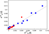 |
Fig. 1. Phase-noise values for the optimal models based on the original O−C curves (σe(1)) and the residuals (σe(2)). The grey line with unit slope illustrates the overall similarity of the two sets. The red symbols correspond to Kepler’s original target stars, and blue rectangles indicate stars found in the background pixels. |
The M3 or M4 model proved to be optimal for 24 original RRab O−C curves, whereas the M2 model was preferred for KPP01. For 13 RRab stars, the residual O−C curves were best described by the M2 model (phase noise plus C2C variation). This outcome is consistent with expectations, as once the dominant periodic variations caused by the Blazhko effect are removed, only phase noise and C2C variation should remain. In five cases, the residual curves were still best fitted by the M4 model. This may indicate that the Blazhko-related period variation was not entirely removed or that a separate long-term period variation is present. The same explanation applies to the four stars whose residuals were dominated by real period variations (M3). For the three stars where the residuals were best fitted by the M1 model, the high noise level likely masked any detectable C2C variation. No residuals were constructed for the two RRc stars (KPP14 and KPP15), and their original O−C diagrams are described by the M2 and M4 models.
The parameters σe(1), ση(1), and σξ(1) obtained from the optimal models of the original O−C diagrams are listed in Columns 8–10 of Table A.2, while the corresponding values for the residuals, σe(2), ση(2), and σξ(2), are given in Columns 11–13. The IDs of the optimal models for both the original and residual O−C diagrams are shown in Column 14.
As Benkő et al. (2025) found a correlation between the strength of the C2C variation (ση) and the pulsation period for non-Blazhko stars, we examined whether a similar relationship exists for Blazhko stars. The upper-left panel of Fig. 2 presents the ση(1) values obtained from the original O−C curves of RRab stars. Due to the large range of values, a logarithmic vertical scale was used. Comparison between Blazhko and non-Blazhko stars showed that (i) the ση(1) values are significantly higher than those of the non-Blazhko RRab stars (grey dots in the figure) and that (ii) no clear dependence on the period is apparent.
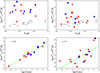 |
Fig. 2. Dependence of the ση parameter characterising the C2C variation in RRab stars on the pulsation period P0 and the strength of the FM part of the Blazhko effect R. Based on the original O−C curves (left) and calculated from the residuals (right). Grey dots represent the sample of non-Blazhko stars from Benkő et al. (2025). Green lines show linear fits; r denotes the Pearson correlation coefficient. Red dots correspond to Kepler’s original targets, and blue rectangles correspond to background stars. |
The upper-right panel of Fig. 2 shows the period dependence of the ση(2) values obtained from the residual O−C diagrams. Although some values fall within the range observed for non-Blazhko stars, the mean value, ⟨ση(2)⟩ = 7.18 × 10⁻⁴, remains higher than that for non-Blazhko RRab stars (⟨ση(RRab)⟩ = 1.76 × 10⁻⁵) and RRc stars (⟨ση(RRc)⟩ = 1.20 × 10⁻⁴). No evident period dependence was observed in this case either.
To quantify the strength of the FM component of the Blazhko effect as reflected in the O−C diagrams, we introduced the parameter
 (3)
(3)
where Ai are the amplitudes (in minutes) of the frequencies associated with the Blazhko effect in the O−C spectrum. The term R serves as a global index of the strength and complexity of the FM modulation since it increases when additional harmonics or combination peaks are present or when their amplitudes are larger.
The lower-left panel of Fig. 2 shows ση(1), which characterises the strength of the C2C variation, plotted against the R parameter representing the strength of the Blazhko FM component. A very strong correlation is evident, with a Pearson correlation coefficient of r = 0.973. In the figure, a similar plot for the residuals (lower-right panel) reveals a slightly weaker but still strong correlation (r = 0.701). This effect likely reflects that part of the Blazhko variation is absorbed into the ση(1) term when fitting the original O−C curves, whereas the residuals isolate the intrinsic C2C component.
This finding suggests that the C2C variation and the Blazhko effect are interrelated, although the physical nature of this relationship is unclear. At this stage, it remains unclear whether the Blazhko effect amplifies the C2C variation, whether strong C2C variability contributes to the occurrence of the Blazhko effect, or whether both phenomena arise from a common underlying cause – or even coincide by chance. A definitive conclusion would require a theoretical explanation both for the origin of the C2C variation and for the mechanism of the Blazhko effect, which is currently lacking.
4. Conclusions
In this letter, we have investigated the C2C variations of RR Lyrae stars showing the Blazhko effect using the same statistical approach previously applied to non-Blazhko stars (Benkő et al. 2025). Benkő et al. (2025) demonstrated that the irregular O−C variations observed in most non-Blazhko RR Lyrae stars can be explained as the consequence of random C2C fluctuations in their light curves.
Based on our work, we arrive at a similar conclusion, finding that the M2 and M4 models (both incorporating C2C variation) provide the optimal description for the O−C curves of 20 stars in our 27-object sample. The parameter ση, which characterises the strength of the C2C variation, is on average larger for Blazhko stars than for both non-Blazhko RRab and RRc stars. This result qualitatively explains why Blazhko stars tend to exhibit stronger irregular O−C variations than non-Blazhko ones. The strength of the FM component of the Blazhko effect shows a clear positive correlation with the C2C variation strength, as a stronger Blazhko effect corresponds to a larger ση value. As a by-product of our analysis, we identified two background RR Lyrae stars (KPP14 and KPP23) in the original Kepler field showing clear phase variations, and we propose them as new Blazhko candidates. Overall, these results demonstrate that incorporating C2C variability is essential for a physically meaningful interpretation of the O−C behaviour of both Blazhko and non-Blazhko RR Lyrae stars.
Acknowledgments
This paper includes data collected by the Kepler mission. Funding for the mission is provided by the NASA Science Mission Directorate. The research was partially supported by the ‘SeismoLab’ KKP-137523 Élvonal grant of the Hungarian Research, Development and Innovation Office (NKFIH) Some PYTHON codes were developed with the help of ChatGPT 5.0
References
- Benkő, J. M., Plachy, E., Szabó, R., Molnár, L., & Kolláth, Z. 2014, ApJS, 213, 31 [CrossRef] [Google Scholar]
- Benkő, J. M., Jurcsik, J., & Derekas, A. 2019, MNRAS, 485, 5897 [CrossRef] [Google Scholar]
- Benkő, J. M., Bódi, A., Plachy, E., & Molnár, L. 2025, A&A, 697, A154 [NASA ADS] [CrossRef] [EDP Sciences] [Google Scholar]
- Borucki, W. J., Koch, D., Basri, G., et al. 2010, Science, 327, 977 [Google Scholar]
- Catelan, M. 2009, Ap&SS, 320, 261 [Google Scholar]
- Forró, A., Szabó, R., Bódi, A., & Császár, K. 2022, ApJS, 260, 20 [CrossRef] [Google Scholar]
- Hajdu, G., Pietrzyński, G., Jurcsik, J., et al. 2021, ApJ, 915, 50 [NASA ADS] [CrossRef] [Google Scholar]
- Hertzsprung, E. 1919, Astron. Nachr., 210, 17 [Google Scholar]
- Jurcsik, J., & Smitola, P. 2016, Commmun. Konkoly Obs. Hungary, 105, 167 [Google Scholar]
- Jurcsik, J., Hajdu, G., Szeidl, B., et al. 2012, MNRAS, 419, 2173 [NASA ADS] [CrossRef] [Google Scholar]
- Koen, C. 2006, MNRAS, 365, 489 [Google Scholar]
- Kovács, G. 2016, Commmun. Konkoly Obs. Hungary, 105, 61 [NASA ADS] [Google Scholar]
- Le Borgne, J. F., Paschke, A., Vandenbroere, J., et al. 2007, A&A, 476, 307 [EDP Sciences] [Google Scholar]
- Lenz, P., & Breger, M. 2005, Commun. Asteroseismol., 146, 53 [Google Scholar]
- Netzel, H., Smolec, R., Soszyński, I., & Udalski, A. 2018, MNRAS, 480, 1229 [NASA ADS] [Google Scholar]
- Plachy, E., Benkő, J. M., Kolláth, Z., Molnár, L., & Szabó, R. 2014, MNRAS, 445, 2810 [Google Scholar]
- Prudil, Z., Skarka, M., Liška, J., Grebel, E. K., & Lee, C.-U. 2019, MNRAS, 487, L1 [CrossRef] [Google Scholar]
- Skarka, M., Prudil, Z., & Jurcsik, J. 2020, MNRAS, 494, 1237 [NASA ADS] [CrossRef] [Google Scholar]
- Smolec, R. 2016, in 37th Meeting of the Polish Astronomical Society, 3, 22 [Google Scholar]
- Sterken, C. 2005, ASP Conf. Ser., 335, 3 [Google Scholar]
- Szeidl, B., Hurta, Z., Jurcsik, J., Clement, C., & Lovas, M. 2011, MNRAS, 411, 1744 [Google Scholar]
Appendix A: O−C diagrams of Blazhko RR Lyrae stars in the original Kepler field
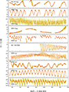 |
Fig. A.1. O−C diagrams of Kepler Blazhko RR Lyrae stars prepared using the template-fitting method. Red curves represent the main target stars of the Kepler mission, for which the light curves were taken from Benkő et al. (2014). The blue curves represent stars found by Forró et al. (2022) in the background pixels. There can be a difference of four orders of magnitude in the O−C values of individual stars (see vertical scales). The light yellow bars show estimated errors based on a Monte Carlo simulation. |
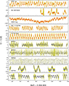 |
Fig. A.1. Continued. |
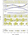 |
Fig. A.1. Continued. The last panel shows KPP26, in which Forró et al. (2022) found uncertain amplitude variations in addition to KPP23. |
Pre-whitened frequencies of the O−C diagrams.
Kepler Blazhko RR Lyrae stars to whose O−C diagrams we fitted statistical models.
All Tables
Kepler Blazhko RR Lyrae stars to whose O−C diagrams we fitted statistical models.
All Figures
|
Fig. 1. Phase-noise values for the optimal models based on the original O−C curves (σe(1)) and the residuals (σe(2)). The grey line with unit slope illustrates the overall similarity of the two sets. The red symbols correspond to Kepler’s original target stars, and blue rectangles indicate stars found in the background pixels. |
| In the text | |
|
Fig. 2. Dependence of the ση parameter characterising the C2C variation in RRab stars on the pulsation period P0 and the strength of the FM part of the Blazhko effect R. Based on the original O−C curves (left) and calculated from the residuals (right). Grey dots represent the sample of non-Blazhko stars from Benkő et al. (2025). Green lines show linear fits; r denotes the Pearson correlation coefficient. Red dots correspond to Kepler’s original targets, and blue rectangles correspond to background stars. |
| In the text | |
|
Fig. A.1. O−C diagrams of Kepler Blazhko RR Lyrae stars prepared using the template-fitting method. Red curves represent the main target stars of the Kepler mission, for which the light curves were taken from Benkő et al. (2014). The blue curves represent stars found by Forró et al. (2022) in the background pixels. There can be a difference of four orders of magnitude in the O−C values of individual stars (see vertical scales). The light yellow bars show estimated errors based on a Monte Carlo simulation. |
| In the text | |
|
Fig. A.1. Continued. |
| In the text | |
|
Fig. A.1. Continued. The last panel shows KPP26, in which Forró et al. (2022) found uncertain amplitude variations in addition to KPP23. |
| In the text | |
Current usage metrics show cumulative count of Article Views (full-text article views including HTML views, PDF and ePub downloads, according to the available data) and Abstracts Views on Vision4Press platform.
Data correspond to usage on the plateform after 2015. The current usage metrics is available 48-96 hours after online publication and is updated daily on week days.
Initial download of the metrics may take a while.