| Issue |
A&A
Volume 705, January 2026
|
|
|---|---|---|
| Article Number | A134 | |
| Number of page(s) | 11 | |
| Section | Stellar atmospheres | |
| DOI | https://doi.org/10.1051/0004-6361/202557640 | |
| Published online | 16 January 2026 | |
KOALA, a new ATLAS9 database
I. Model atmospheres, opacities, fluxes, bolometric corrections, magnitudes, and colours
1
Dipartimento di Fisica e Astronomia “Augusto Righi”, Alma Mater Studiorum, Università di Bologna,
Via Gobetti 93/2,
40129
Bologna,
Italy
2
INAF – Osservatorio di Astrofisica e Scienza dello Spazio di Bologna,
Via Gobetti 93/3,
40129
Bologna,
Italy
3
LIRA, Observatoire de Paris, Université PSL, Sorbonne Université, Université Paris Cité, CY Cergy Paris Université, CNRS,
92190
Meudon,
France
4
INAF – Osservatorio Astronomico di Trieste,
Via G.B.Tiepolo 11,
Trieste
34143,
Italy
★ Corresponding author: This email address is being protected from spambots. You need JavaScript enabled to view it.
Received:
10
October
2025
Accepted:
12
November
2025
Abstract
We present the KOALA database, a new set of local thermodynamic equilibrium line-blanketed model atmospheres calculated with the code ATLAS9, together with the corresponding opacity distribution functions and emergent fluxes. The latter were also used to calculate G-band bolometric corrections and theoretical magnitudes and colours for several photometric systems, i.e. UBVRI, 2MASS, Hypparcos-Tycho, SDSS, Galex, Euclid, and Gaia DR3. With respect to previous grids of ATLAS9 model atmospheres, we adopted the solar mixture by Caffau/Lodders, and we extend the sampling in metallicity (from −5.0 to −2.5 dex, with a step of 0.5 dex, and from −2.5 dex to +0.5 dex, with a step of 0.25 dex) and in [α/Fe] (from −0.4 to +0.4 dex, with a step of 0.2 dex). We also provide a finer sampling in Teff for Teff lower than 7000 K. This finer grid allows for more accurate interpolation of colours, and in many cases it makes computing a new model atmosphere unnecessary since the atmosphere of the grid can be used directly. We computed a total of 51 663 model atmospheres and emergent fluxes. Finally, we discuss the impact of [M/H] and [α/Fe] on the thermal and pressure structures of the model atmospheres and on theoretical colours.
Key words: stars: atmospheres
© The Authors 2026
 Open Access article, published by EDP Sciences, under the terms of the Creative Commons Attribution License (https://creativecommons.org/licenses/by/4.0), which permits unrestricted use, distribution, and reproduction in any medium, provided the original work is properly cited.
This article is published in open access under the Subscribe to Open model. This email address is being protected from spambots. You need JavaScript enabled to view it. to support open access publication.
1 Introduction
A model atmosphere describes how thermodynamic quantities (i.e. temperature, gas pressure, electron number density) vary when moving through the photosphere from outer optically thin layers to the deeper optically thick regions, where continuum photons are formed. The change of these quantities with the depth can be expressed as a function of the optical depth (in plane-parallel geometry) or of the stellar radius (in spherical geometry). The model atmospheres are the backbone of the spectral synthesis and of the spectral energy distribution modelling of stars observed at different resolutions through photometric filters or spectra. In astrophysics, model atmospheres are a fundamental element in chemical abundance analysis, in the transformation of stellar tracks and isochrones into observational planes, and in the spectral energy distribution modelling of galaxies.
The only publicly available codes to calculate model atmospheres are ATLAS9 (Kurucz 1970; Kurucz et al. 1974; Kurucz 2005) and ATLAS12 (Kurucz 2005; Castelli 2005b) as well as TLUSTY (Hubeny 1988; Hubeny & Lanz 1995; Lanz & Hubeny 2003) and TMAP (Werner & Dreizler 1999). However, there are other codes that are not publicly distributed, despite the wide use of their grids of model atmospheres, including MARCS (Gustafsson et al. 2008) and PHOENIX (Hauschildt et al. 1997; Hauschildt & Baron 1999). With respect to other codes that are suitable for specific regions of a parameter space, i.e. TLUSTY for OB stars (but usable also for cooler stars, see e.g. Hubeny et al. 2021), MARCS for FGKM stars, and PHOENIX for AFGKM stars, ATLAS9 and ATLAS12 allow reliable model atmospheres to be calculated over a large range of parameters. These models assume one-dimensional plane-parallel geometry, local thermodynamic and radiative equilibrium, and radiation and convection as the only energy transport mechanisms. The main difference between ATLAS9 and ATLAS12 is in the treatment of the line opacity. ATLAS9 handles the complex and time-consuming step of calculating the line opacity coefficient using the opacity distribution function (ODF) method (see Kurucz 1979, and references therein). In this approach, the line opacity for a given chemical mixture and microturbulent velocity (vturb) is calculated as a function of temperature and gas pressure in a number of wavelength intervals, namely, 328 intervals for the so-called big ODF (used in the model atmosphere calculation) and 1212 for the so-called little ODF (used in the emergent flux calculation).
The main advantage of the ODF method is that after a relatively time-consuming effort of calculating big and little ODFs, any model atmosphere or emergent flux with the chemical mixture and vturb of the corresponding ODF can be calculated in a very short time when adopting the appropriate Teff and log g. This approach is therefore suitable to calculate a large number of models and emergent fluxes for stars with a similar chemical composition. For stars with peculiar chemical compositions (or with specific elemental abundances that significantly impact the total opacity), the opacity sampling method (Peytremann 1974, and implemented in ATLAS12) is recommended, as it allows for proper calculation of the opacity coefficients for the parameters of the model.
The availability of extensive grids of atmospheric models (as well as ODFs and fluxes) that adequately sample the parameter space (not only Teffand log gbut also the chemical mixture) is fundamental for various aspects of astrophysics. The most used grids of ATLAS9 model atmospheres have been provided by Castelli & Kurucz (2003, hereafter CK03)1. This grid assumes a reference solar mixture by Grevesse & Sauval (1998), and it provides metallicities [M/H] between −4.0 and +0.5 dex, with a typical step of 0.5 dex, and two values of [α/Fe], +0.0 and +0.4 dex. However, the grid is not sampled in a regular way due to lacking some combination of [M/H] and [α/Fe].
With this work, we present the first paper of the KOALA project. KOALA is a new database of opacities, model atmospheres, and emergent fluxes calculated with the ATLAS9 software. In this paper we describe the new grid that substitutes the previous ones by CK03 and follows the same physical assumptions, particular those for the adopted opacities. In subsequent papers, we will discuss future grid testing and the impact of peculiar chemical composition and of some physical assumptions.
2 The new ATLAS9 grid
We present a new, wider, and more complete grid of ODFs, model atmospheres, and emergent fluxes, calculated with the gfortran version of the codes DFSYNTHE, KAPPA9 (Castelli 2005a), and ATLAS9 (Kurucz 2005). All codes are available in the F. Castelli website2. With respect to the grid by CK03, we adopted a different solar chemical composition, we increased the parameter sampling in [M/H] and [α/Fe], and we increased the sampling in Teff for the cool models (see details in Sect. 2.1). All the products of this new release (big and little ODFs, Rosseland opacity tables, model atmospheres, emergent fluxes, G-band bolometric corrections, and theoretical magnitudes) are available at a dedicated website3, where we will also provide new grids of models calculated with specific chemical mixtures or the testing of different physical assumptions. The dataset presented here has already been used to calculate the colour-temperature transformations used to transform the theoretical isochrones and tracks of the BaSTI-IAC database4 into observational planes (Hidalgo et al. 2018; Pietrinferni et al. 2021, 2024).
2.1 Main features and novelties
In this section, we summarise the characteristics of this new grid. We also discuss the main improvements with respect to the previous grid by CK03.
The reference solar chemical mixture is composed of the solar abundances by Caffau et al. (2011) for Li, C, N, O, P, S, K, Fe, Eu, Hf, Os and Th, and those by Lodders (2010) are used for the other elements. This new solar chemical mixture substitutes the one by Grevesse & Sauval (1998) adopted by CK03. For all the ODFs, we assumed a helium mass fraction of Y=0.2476, following the Planck mission results (Coc et al. 2014). We point out that the relatively small change in He abundance due to the Galactic chemical evolution has minor effects on the structure of the model atmospheres. For a detailed description on the effects of the He abundance on the spectra of late-type stars, we refer to Böhm–Vitense (1979).
We considered different chemical mixtures in terms of α-elements (O, Ne, Mg, Si, S, Ar, Ca, and Ti), namely, [α/Fe]=−0.4, −0.2, +0.0, +0.2 and +0.4 dex. The grid by CK03 included only [α/Fe]=+0.0 and +0.4 dex.
For each value of [α/Fe], we considered 18 metallicities. The adopted metallicities range from [M/H]=−5.0 dex to −2.5 dex with a step of 0.5 dex, and from −2.5 dex and +0.5 dex, with a step of 0.25 dex. This significantly extends the metallicity range and sampling of the grid by CK03, which adopted a sampling of +0.5 dex and lacked some metallicities for [α/Fe]=+0.4 dex. Therefore, for each [α/Fe] we provide a regular grid of models in terms of [M/H].
Another novelty of the new grid with respect to the grid by CK03 is the adoption of a step of 125 K in the range 3750–6000 K (for log g≤3.0) and in the range 3750–7000 K (for log g>3.0). This makes our grid finer by a factor of two with respect to the grid by CK03. This finer grid allows for more accurate interpolation of colours, and in many cases it makes computing a new model unnecessary since one of the grids can be used directly. We added as a boundary of the grid, models with Teff=3750 K, even if problems in the ATLAS9 integrated colours for Teff lower than 4000 K have been identified (see e.g. Plez 2011). For hotter Teff, we maintain the same step by CK03: 250 K for stars up to Teff =12 000 K, 500 K up to Teff =20 000 K, and 1000 K up to Teff =50 000 K. For log g we also adopted the same step (0.5 dex) by CK03. Figure 1 shows the sampling of the entire grid in the Teff-log g plane compared with the extension of the MARCS (Gustafsson et al. 2008), PHOENIX (Husser et al. 2013), and TLUSTY (Lanz & Hubeny 2003, 2007) model atmospheres.
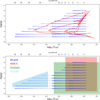 |
Fig. 1 Distribution of the ATLAS9 model atmospheres of the new grid (blue circles) in the log10(Teff)–log g plane superimposed (upper panel) to four theoretical BaSTI-IAC isochrones with 15 Myr, 100 Myr, 1 Gyr, and 13 Gyr and a solar-scaled metallicity (Hidalgo et al. 2018) and compared (lower panel) to the distribution of MARCS (Gustafsson et al. 2008), PHOENIX (Husser et al. 2013), and TLUSTY (Lanz & Hubeny 2003, 2007) model atmospheres. |
Number of computed model atmospheres and fluxes according to the metallicity and [α/Fe].
2.2 Calculation of ODFs, model atmospheres, and emergent fluxes
The ODFs were computed with DFSYNTHE and KAPPA9 codes (Castelli 2005a), adopting the same atomic and molecular line lists used by CK03 and described in Kurucz (2011). We briefly note that in the computation of the ODFs, we included all the atomic lines in the last release of the R. L. Kurucz dataset as well as the linelists for several diatomic molecules, i.e. H2, CH, NH, OH, MgH, SiH, C2, CN, CO, SiO, and TiO (we adopted the TiO linelists by Schwenke 1998). The only difference with respect to the opacities used by CK3 is related to H2O. For H2O we adopted the last version of the Partridge & Schwenke (1997) linelist as provided by R. L. Kurucz5, which has had a bug present in the previous release of the same linelist fixed. In the future releases of KOALA, we plan to provide improvements on new opacity sources not included in the last release of Kurucz’s database. For each chemical composition, specified by the metallicity [M/H] (see Appendix A) and the α-element abundance ratio [α/Fe], we calculated big and little ODFs by adopting five values of vturb: 0, 1, 2, 4, and 8 km/s.
Model atmospheres with vturb=2 km/s were calculated with ATLAS9 (Kurucz 2005), adopting the big ODFs. ATLAS9 enforces Saha–Boltzmann ionisation-excitation plus molecular dissociation equilibrium at each depth together with elemental abundance conservation and charge neutrality. The code solves a coupled set of equilibrium equations for all species (atoms and ions and selected molecules), returning number densities and the electron pressure for a given temperature, pressure, and composition. For additional details about the main physical assumptions and the calculation scheme adopted by ATLAS9, we refer to the vast literature available on this code (Kurucz 1970; Kurucz et al. 1974; Kurucz 1979; Castelli 1988).
Since a model atmosphere is calculated through an iterative numerical process starting from a guess solution, these models were obtained by choosing as the guess model the CK03 grid model closest in terms of Teff, log g, and [M/H] to the solution to be computed. The choice of a different guess model, as long as it is close to the desired solution, has a negligible impact on the computed model, whereas using guess models that are far from the required solution can slow down the calculation or compromise the convergence of the final model.
All of the models have 72 plane-parallel layers ranging from the logarithm of the Rosseland optical depth log τRoss=−6.875 to +2.00, in steps of δlog τRoss = 0.125. In the treatment of the convective flux, the classical mixing length theory (Böhm–Vitense 1953; Böhm-Vitense 1958) was adopted, with the pressure scale height equal to α times the characteristic length of a rising convective cell. We adopted a mixing length parameter α equal to 1.25, as done in previous grids of ATLAS9 models (CK03, Kirby 2011; Mészáros et al. 2012). We stress that the adoption of a different value only impacts the deepest layers of the coolest models, where continuum and very weak lines form. The approximate overshooting (Kurucz 1992) was switched off because even if it is able to better reproduce some spectral features in the solar spectrum, for most of the stars it does not provide a good description of several features (Castelli et al. 1997), and it introduces unphysical features in the thermal structure of the most metal-poor models (Bonifacio et al. 2009). For all the layers, local thermodynamical equilibrium was assumed (but this assumption can becomes progressively less realistic for temperatures hotter than ~15 000 K, see e.g. Lanz & Hubeny 2007).
For any model, a given layer was considered converged if its flux and flux-derivative errors were less than 1 and 10%, respectively. The majority of the computed models satisfy these criteria in all the layers. In some models (especially those with low Teff and log g), some layers are not converged, usually the most external ones. Sometimes, small changes in the guess model atmosphere (e.g. of the order of some tens of K) can be enough to solve the problems of the convergence of a layer. However, possible non-converged outermost layers do not significantly affect the use of the model atmosphere because in those layers, the core of the strong lines formed, which are usually not adopted for chemical analyses because of some effects (i.e. non-local thermodynamic equilibrium, chromospheric activity) are not accounted for in ATLAS models. Additionally, for some low Teff(≲4600), high log g (≥2.0–2.5), and low [M/H] models ([M/H]<−2.5 dex, i.e. models corresponding to metal-poor, low main sequence stars, such as K and M dwarfs), we found problems of convergence also in the central layers, where a significant fraction of the flux is transported by convection (in particular an unphysical discontinuity in temperature is present close to these layers). The use of different guess model atmospheres or small changes in the requested parameters were not able to fix this issue, and we decided to remove these models from the grid.
The number of model atmospheres of the final grid is summarised in Table 1, according to the adopted [M/H] and [α/Fe]. A total of 51 663 model atmospheres are provided. Finally, for each model in the grid described above, the corresponding emergent flux (i.e. a low-resolution spectrum covering the entire spectral range) was calculated as the energy per frequency unit, Hν.
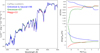 |
Fig. 2 Left panel: comparison among ATLAS9 fluxes for the Sun calculated with suitable ODFs adopting different solar chemical mixtures: Caffau-Lodders (this work, grey line), Grevesse & Sauval (1998, blue line), Grevesse et al. (2007, green line), and Magg et al. (2022, red line). Right panels: percentage difference in temperature (upper panel) and logarithm of the gas pressure (lower panel) as a function of the Rosseland optical depth of the model atmospheres with respect to that computed with Caffau-Lodders chemical mixture (same colour-code as the left panel). |
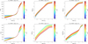 |
Fig. 3 Run of temperature (left panels), logarithm of the gas pressure (middle panels), and logarithm of the electron number density (right panels) as a function of log τRoss for the model atmospheres of a dwarf star (Teff=6500 K and log g=4.5, upper panels) and a giant star (Teff=4500 K and log g=1.5, lower panels). The colour-coding is according to the metallicity of [M/H]. We adopted [α/Fe]=+0.0 dex for all the models. |
3 Impact of the adopted solar chemical mixture
Making a comparison between the different families of the model atmospheres is not trivial because of the large number of assumptions in the recipes adopted by different codes. In order to evaluate the true impact of the different solar chemical mixtures on the model atmospheres and fluxes, we calculated additional ODFs, assuming the solar mixtures by Grevesse & Sauval (1998), used by CK03, Grevesse et al. (2007), used in the MARCS models grid by Gustafsson et al. (2008), and the recent solar chemical composition by Magg et al. (2022). The most significant differences among these four mixtures are for C, N, and O. In Fig. 2 we compare the emergent fluxes and the thermal and pressure structures of the model atmospheres for the Sun while adopting these chemical mixtures. Small differences are appreciable in the outermost regions, especially for the model adopting the mixture by Grevesse et al. (2007), characterised by the lowest C, N, and O abundances. This exercise suggests that the adoption of the solar chemical mixture does not significantly impact the structure of the model atmospheres. On the other hand, the adopted solar abundances have a significant impact on the derived fluxes in the UV/blue spectral regions dominated by strong CH, NH, and CN molecular bands. Checks we performed for other sets of metallicity and stellar parameters led to similar conclusions.
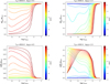 |
Fig. 4 Run of a fraction of electrons provided by H (upper panels) and Mg (lower panels) as a function of log τRoss for the model atmospheres of a dwarf (Teff=6500 K and log g=4.5, left panels) and a giant star(Teff=4500 K and log g=1.5, right panels). The colour-coding is according to the metallicity of [M/H]. We adopted [α/Fe]=+0.0 dex for all the models. |
4 Impact of the metallicity on the model atmospheres
In Fig. 3, we show how the model atmospheres for a giant star (Teff=4500 K and log g=1.5) and for a dwarf (Teff=6500 K and log g=4.5) star change by changing [M/H]. In particular, we show the run of temperature, gas pressure (log(Pgas)), and electron number density (log(XNelec)) as a function of log τRoss. Based on the figure, it is immediately clear that models with [M/H]≳−2.5/−2.0 dex become increasingly distinct from each other at a fixed optical depth, while models that are more metal poor are often indistinguishable or show only small differences. This justifies our choice of a finer sampling at higher metallicities, namely, +0.25 instead of the +0.5 adopted by CK03. As an exercise, we discuss in Appendix B the properties of a zero-metallicity ODF representative of an ideal Population III star.
The thermal structure of the model is sensitive to [M/H], especially in deeper (log τRoss≳0.5) and outer (log τRoss≲−3) layers (with the differences more pronounced in the giant model). When fixing Teff (and therefore the total flux, according to the Stefan-Boltzmann relation), a higher metallicity leads to a larger absorption from metallic lines and a higher opacity. This reduces the capability of the star to radiate energy, and the temperature of the innermost layers must therefore increase to make the total flux constant. On the other hand, the temperature of the outermost layers (where the atmosphere becomes optically thin) decreases because it is easier for the model to radiate energy (see e.g. Kurucz 1979).
The gas pressure and the electron number density are also significantly affected by [M/H], but in different and opposite ways. For [M/H]≳−3.0/−2.5 dex, log(Pgas) increases by decreasing [M/H] at each log τRoss, while log(XNelec) decreases. This occurs because as the metallicity decreases, the fraction of free electrons (provided by metals) also decreases, leading to a lower electron number density (right panels of Fig. 3) and therefore a lower number of H− atoms. This corresponds to a lower line opacity coefficient that increases the gas pressure according to the hydrostatic equilibrium (middle panels of Fig. 3) even if the electron pressure decreases.
For [M/H]≲−3.0 dex, the gas pressure and the electron number density are very similar despite different metallicities in most of the model. In the outermost layers, the metal-poor models have steeper gas pressures and a higher electron number density. This behaviour reflects the different contributor to free electrons provided by hydrogen and metals in the outermost layers of metal-poor atmospheres. As shown in Fig. 4, which shows the fraction of electrons provided by H and Mg as a function of log τRoss, in the external regions and where [M/H]<−3.0 dex, hydrogen becomes the dominant source of free electrons, while the contributor of Mg (the main electron donor for FGK stars) decreases significantly.
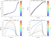 |
Fig. 5 Model atmospheres with Teff =4500 K, log g=1.5, [M/H]=+0.0 dex, and different [α/Fe]values. The panels show the behaviour of the temperature, logarithm of the gas pressure, and fractions of free electrons provided by Mg and Fe. The model with [α/Fe]=−0.4 dex, which shows a different behaviour with respect to the other models, is plotted with a thicker curve. |
5 Impact of the adopted [α/Fe] on the model atmospheres
The approach commonly used when computing a synthetic spectrum is to vary the abundance of a given element while still using an atmospheric model that was calculated with a different abundance for that species. This procedure is legitimate and does not introduce significant errors as long as the abundance variations do not have a major impact on the atmospheric opacity or the ionisation structure. Therefore, even substantial changes in the abundances of elements that contribute little to the overall opacity do not lead to inaccuracies in the resulting synthetic spectrum. On the other hand, greater caution should be exercised when varying the abundances of elements such as the α elements. Therefore, the use of model atmospheres including appropriate chemical mixtures in terms of [α/Fe] is recommended.
We checked the differences in the thermal and pressure structures of model atmospheres with different [α/Fe]. We recognised a peculiar pattern in cool models with [M/H]≳−2.0 dex and [α/Fe]=−0.4 dex. As visible in Fig. 5, the decrease of [α/Fe] at a fixed [M/H] mimics a decrease of [M/H] with the features that we discussed in Sect. 4. On the other hand, the model with [α/Fe]=−0.4 dex is discrepant in the outermost layers, where it has a higher Teff and a lower lower Pgas than the model with [α/Fe]=−0.2 dex (we would expect the opposite behaviour following Fig. 3). This run could be explained by the peculiar chemical mixture of this model, where the extremely low [α/Fe] changes the budget of the free electrons. In fact, we found that the free electrons in the outermost layers of this model arise mainly from Fe and Mg, both negligible in the external regions of the other models, where the majority of the free electrons are provided by Na and Al.
A finer sampling of [α/Fe] in the adopted model atmospheres also has an impact on the spectral synthesis, particularly on the strength of some specific features sensitive to the adopted chemical mixture of the model atmosphere. An example of possible issues arising from the use of model atmospheres with different [α/Fe] values is visible in the analysis of the Ca II triplet lines. Figure 6 shows a comparison between synthetic spectra of the second Ca II triplet line calculated with the code SYNTHE and using our new grid of model atmospheres. In particular, the three synthetic spectra were calculated with the same Ca abundance ([Ca/Fe]=+0.2 dex) but assuming three different model atmospheres in terms of [α/Fe], namely, +0.0, +0.2, and +0.4 dex. This means that in the spectral synthesis calculation, we varied the Ca abundance of +0.2, 0.0, and −0.2 dex with respect to the original abundance of the models, respectively, in order to obtain the same [Ca/Fe]. Despite the same Ca abundance of the three synthetic spectra, the wings of the Ca II line are different from each other. The broadening of these lines is dominated by van der Waals broadening and extremely sensitive to the gas pressure. The increase of [α/Fe] in the model atmosphere (despite the Ca abundance variation adopted in the spectral synthesis) leads to a decrease of the gas pressure (similar to what happens when [M/H] increases), reducing the strength of the wings. On the other hand, linear and saturated Ca lines are not affected by the assumption of the [α/Fe] of the model atmosphere.
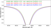 |
Fig. 6 Synthetic spectra for the second line of the Ca II triplet calculated with model atmospheres with Teff=4500 K, log g=1.5, [M/H]=+0.0 dex, and three different values of [α/Fe]. Despite the latter value, all the synthetic spectra were computed assuming [Ca/Fe]=+0.2 dex. |
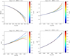 |
Fig. 7 Upper-left panel: run of the G-band bolometric correction as a function of Teff for model atmospheres with log g=1.5, [M/H]=+0.0 dex and different values of [α/Fe]. Upper-right panel: run of (V-I) as a function of Teff (log g=4.5, [M/H]=+0.0 dex). Lower-left panel: run of (B-V) as a function of Teff (log g=4.5, [M/H]=+0.0 dex). Lower-right panel: run of (J-K) as a function of Teff (log g=1.5, [M/H]=+0.0 dex). |
6 Theoretical magnitudes and colours
For each flux of the new grid described above we calculated the theoretical magnitudes and colours in different photometric systems and bolometric corrections in the Gaia DR3 G-band, BC(G). The procedure to calculate the theoretical colours is described in detail in Appendix C. The photometric systems that we considered are the UBVRI (Bessell & Murphy 2012), the 2MASS JHK (Cohen et al. 2003), the Hipparcos-Tycho (Bessell & Murphy 2012), the SDSS ugriz (Fukugita et al. 1996), the Euclid IEYEJEHE (Euclid Collaboration: Schirmer et al. 2022), the GALEX NUV and FUV (Morrissey et al. 2007), and the Gaia DR3 photometric system (Gaia Collaboration 2023).
The behaviour of bolometric corrections and colours as a function of the parameters (i.e. Teff, log g, and [M/H]) has been extensively discussed in other works (see e.g. Bessell et al. 1998; Bonifacio et al. 2018; Casagrande & VandenBerg 2018). Here we focus on their sensitivity regarding the adopted [α/Fe], the main novelty of this new dataset. The G-band bolometric correction, BC(G), is basically unaffected by the adopted [α/Fe], but for metal-rich ([M/H]≥+0.0 dex) giant models, the BC(G) decreases by increasing [α/Fe]. As an example, Fig. 7 shows the run of BC(G) as a function of Teff for [M/H]=+0.0 dex and different values of [α/Fe].
The sensitivity of BC(G) with [α/Fe] can be appreciated at a lower Teff. At lower metallicities, the difference among the models, even at low Teff, decreases and disappears entirely. Below [M/H]~−1.0 dex, BC(G) is completely independent of [α/Fe] value.
Concerning the colours, the main effects of [α/Fe] appear in general at a low Teff and a high [M/H]. The behaviour of the colours with [α/Fe] at a fixed Teff and [M/H] is not univocal, as it depends on two opposing effects that affect the emerging spectrum when [α/Fe] varies. On one hand, a decrease in [α/Fe] naturally leads to a reduction in the strength of features associated with α-elements, resulting in an increase in flux within the adopted filter profile, especially in the visual region between ~4500 and ~6500 Å and at wavelengths shorter than ~3200 Å. On the other hand, the drop in oxygen alters the molecular equilibrium of the CNO cycle, progressively enhancing the strength of CN molecular bands (see e.g. Ryde et al. 2009) at ~3800 Å and beyond 6500 Åand of the G-band CH band at ~4300 Å. This effect is significantly strong for models with [α/Fe]=−0.4 dex, and therefore the colours calculated with this chemical mixture are in almost all cases the most divergent with respect to the other colours. Figure 8 shows an example of these effects, with two emergent fluxes calculated for a K giant (Teff=4500 K, log g=1.5) and a K dwarf (Teff=4500 K, log g=4.5) star, both with [M/H]=+0.0 dex. In particular, the strong CN and CH molecular features are clearly visible in the emergent fluxes with [α/Fe]=−0.4 dex.
Depending on the filters involved, these two effects can lead to either an increase or a decrease in the flux ratio as [α/Fe] decreases. We grouped the colours into three classes according to their sensitivity on the adopted [α/Fe]:
Colours directly proportional to [α/Fe]: most of the colours become bluer when reducing [α/Fe]. Among them are (r-i), (i-z), all the Gaia colours, (V-I) and (IE-YE) both for giant and dwarf models, and (V-K) for dwarf stars. The run of (V-I) with Teff in dwarf models is shown in the lower-right panel of Fig. 7 as an example of this class of colours.
Colours inversely proportional to [α/Fe]: other colours show an opposite behaviour, becoming redder when reducing [α/Fe], such as (BT-VT), (YE-JE), and for dwarf stars (U-B), (B-V), and (u-g). The run of (B-V) with Teff in dwarf models is shown in the lower-right panel of Fig. 7. In these colours, the flux of the second filter is significantly reduced because the filter profile is dominated by the Mg b triplet (see Fig. 8).
Colours (almost or totally) insensitive to [α/Fe]: all the other colours have a negligible or lacking dependence on the adopted [α/Fe]. Almost all the Euclid colours have little or negligible variations with [α/Fe], but for the models with [α/Fe]=−0.4 dex, the colours are significantly discrepant with respect to other ones. The lower-right panel of Fig. 7 shows as example the run of (J-K) with Teff.
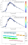 |
Fig. 8 Examples of ATLAS9 emergent fluxes calculated for a giant and dwarf star (upper and middle panel, respectively), calculated with different values of [α/Fe]. The lower panel shows the log-wavelength range of the photometric filters discussed here. |
7 Summary
We have presented a new database of ATLAS9 ODFs, model atmospheres, emergent fluxes, G-band bolometric corrections, and theoretical magnitudes and colours. The latter were calculated in different photometric filters, namely, UBVRI, 2MASS, SDSS, Hypparcos-Tycho, Euclid, Galex, and Gaia DR3. All of the products are available in the dedicated website. The new grid of ODFs includes a finer sampling in [M/H] (from −5.0 to +0.5 dex) and [α/Fe] (from −0.4 to +0.4 dex). We discussed the impact of [M/H] and [α/Fe] on model atmospheres (in terms of temperature, pressure, and electron number density), emergent fluxes, and theoretical colours. Among the features that we discussed, the most relevant are the following:
Models with [M/H]≳−2.5/−2.0 dex become increasingly distinct from each other at a fixed optical depth, in terms of both thermal and pressure structures, while more metal-poor models are often indistinguishable or show only small differences. This highlights the need for a finer sampling in [M/H] for model atmospheres with [M/H]≳−2.5/−2.0 dex.
The thermal structure of the model is sensitive to [M/H], particularly in deeper (log τRoss≳0.5) and outer (log τRoss≲−3) layers. The gas pressure and the electron number density are also significantly affected by [M/H], but in different and opposite ways.
The decrease of [α/Fe] at a fixed [M/H] impacts the thermal and pressure structures of the model atmosphere in a manner similar to the decrease of [M/H]. However, the models with [α/Fe]=−0.4 dex are discrepant in the outermost layers, having higher Teff and lower Pgas than the model with [α/Fe]=−0.2 dex. This is due to the large contribution of Fe and Mg to the budget of the free electrons in outermost layers.
The [α/Fe] in the adopted model atmosphere can affect the spectral synthesis of some features dominated by the van der Waals broadening (e.g. the wings of the Ca II triplet lines). For the spectral synthesis, adopting a model atmosphere with an appropriate chemical composition in terms of [α/Fe]is generally recommended.
-
Theoretical colours can have different sensitivities to [α/Fe]depending on the balance between two different effects affecting the involved filter profiles. A decrease in [α/Fe] leads to weaker α-element features (i.e. the Mg b triplet) and stronger CN and CH features. Again, the colours calculated with [α/Fe]=−0.4 dex are often significantly discrepant with respect to the other colours.
The new grids discussed here significantly expand the previous grid by CK03, providing an useful tool for chemical analyses, photometric studies, theoretical tracks and isochrones. In forthcoming papers, we will present new grids of model atmospheres including peculiar chemical compositions.
Acknowledgements
This work is dedicated to the memory of R. L. Kurucz, who passed away in March 2025 and whose contribution to the study of stellar atmospheres was fundamental. We are grateful to R. Lallement for explaining to us the details of building extinction maps and for reading a draft of our paper. A.M. acknowledges support from the project “LEGO – Reconstructing the building blocks of the Galaxy by chemical tagging” (PI: A. Mucciarelli) granted by the Italian MUR through contract PRIN 2022LLP8TK_001.
References
- Allard, F., & Hauschildt, P. H. 1995, ApJ, 445, 433 [NASA ADS] [CrossRef] [Google Scholar]
- Bessell, M. S. 1990, PASP, 102, 1181 [NASA ADS] [CrossRef] [Google Scholar]
- Bessell, M. S., Castelli, F., & Plez, B. 1998, A&A, 333, 231 [NASA ADS] [Google Scholar]
- Bessell, M., & Murphy, S. 2012, PASP, 124, 140 [NASA ADS] [CrossRef] [Google Scholar]
- Böhm-Vitense, E. 1953, ZAp, 32, 135 [Google Scholar]
- Böhm-Vitense, E. 1958, ZAp, 46, 108 [NASA ADS] [Google Scholar]
- Böhm-Vitense, E. 1979, ApJ, 234, 521 [CrossRef] [Google Scholar]
- Bonifacio, P., Monai, S., & Beers, T. C. 2000, AJ, 120, 2065 [Google Scholar]
- Bonifacio, P., Spite, M., Cayrel, R., et al. 2009, A&A, 501, 519 [NASA ADS] [CrossRef] [EDP Sciences] [Google Scholar]
- Bonifacio, P., Caffau, E., Ludwig, H.-G., et al. 2017, Mem. Soc. Astron. Italiana, 88, 90 [Google Scholar]
- Bonifacio, P., Caffau, E., Ludwig, H.-G., et al. 2018, A&A, 611, A68 [NASA ADS] [CrossRef] [EDP Sciences] [Google Scholar]
- Bonifacio, P., Caffau, E., Sestito, F., et al. 2019, MNRAS, 487, 3797 [CrossRef] [Google Scholar]
- Caffau, E., Ludwig, H.-G., Steffen, M., et al. 2011, Sol. Phys., 268, 255 [NASA ADS] [CrossRef] [Google Scholar]
- Casagrande, L., & VandenBerg, D. A. 2014, MNRAS, 444, 392 [Google Scholar]
- Casagrande, L., & VandenBerg, D. A. 2018, MNRAS, 479, L102 [NASA ADS] [CrossRef] [Google Scholar]
- Castelli, F. 1988, Pubblicazione Osservatorio Astronomico di Trieste, N 1164 [Google Scholar]
- Castelli, F. 1999, A&A, 346, 564 [NASA ADS] [Google Scholar]
- Castelli, F. 2005a, Mem. Soc. Astron. It. Suppl., 8, 34 [Google Scholar]
- Castelli, F. 2005b, Mem. Soc. Astron. It. Suppl., 8, 25 [Google Scholar]
- Castelli, F., & Kurucz, R. L. 2003, IAU Symp., 210, A20 [Google Scholar]
- Castelli, F., Gratton, R. G., & Kurucz, R. L. 1997, A&A, 18, 841 [Google Scholar]
- Coc, A., Uzan, J.-P., & Vangioni, E. 2014, J. Cosmology Astropart. Phys., 10, 050 [CrossRef] [Google Scholar]
- Cohen, M., Wheaton, W. A., & Megeath, S. T. 2003, AJ, 126, 1090 [Google Scholar]
- Danielski, C., Babusiaux, C., Ruiz-Dern, L., et al. 2018, A&A, 614, A19 [NASA ADS] [CrossRef] [EDP Sciences] [Google Scholar]
- Euclid Collaboration (Schirmer, M., et al.) 2022, A&A, 662, A92 [NASA ADS] [CrossRef] [EDP Sciences] [Google Scholar]
- Fitzpatrick, E. L., Massa, D., Gordon, K. D., et al. 2019, ApJ, 886, 108 [NASA ADS] [CrossRef] [Google Scholar]
- Fukugita, M., Ichikawa, T., Gunn, J. E., et al. 1996, AJ, 111, 1748 [Google Scholar]
- Gaia Collaboration (Vallenari, A., et al.) 2023, A&A, 674, A1 [NASA ADS] [CrossRef] [EDP Sciences] [Google Scholar]
- Girardi, L., Grebel, E. K., Odenkirchen, M., et al. 2004, A&A, 422, 205 [NASA ADS] [CrossRef] [EDP Sciences] [Google Scholar]
- Grevesse, N., & Sauval, A. J. 1998, Space Sci. Rev., 85, 161 [Google Scholar]
- Grevesse, N., Asplund, M., & Sauval, A. J. 2007, Space Sci. Rev., 130, 105 [Google Scholar]
- Gustafsson, B., Edvardsson, B., Eriksson, K., et al. 2008, A&A, 486, 951 [NASA ADS] [CrossRef] [EDP Sciences] [Google Scholar]
- Hauschildt, P. H., & Baron, E. 1999, J. Comput. Appl. Math., 109, 41 [NASA ADS] [CrossRef] [Google Scholar]
- Hauschildt, P. H., Baron, E., & Allard, F. 1997, ApJ, 483, 390 [Google Scholar]
- Hidalgo, S. L., Pietrinferni, A., Cassisi, S., et al. 2018, ApJ, 856, 125 [Google Scholar]
- Hill, G. 1982, Pub. Dominion Astrophys. Observ. Victoria, 16, 67 [Google Scholar]
- Hubeny, I. 1988, Comp. Phys. Commun., 52, 103 [NASA ADS] [CrossRef] [Google Scholar]
- Hubeny, I., & Lanz, T. 1995, ApJ, 439, 875 [Google Scholar]
- Hubeny, I., Allende Prieto, C., Osorio, Y., et al. 2021, arXiv e-prints [arXiv:2104.02829] [Google Scholar]
- Husser, T.-O., Wende-von Berg, S., Dreizler, S., et al. 2013, A&A, 553, A6 [NASA ADS] [CrossRef] [EDP Sciences] [Google Scholar]
- Kirby, E. N. 2011, PASP, 123, 531 [NASA ADS] [CrossRef] [Google Scholar]
- Kurucz, R. L. 1970, SAO Special Report, Atlas: a Computer Program for Calculating Model Stellar Atmospheres, 309 [Google Scholar]
- Kurucz, R. L. 1979, ApJS, 40, 1 [NASA ADS] [CrossRef] [Google Scholar]
- Kurucz, R. L. 1992, The Stellar Populations of Galaxies, Model Atmospheres for Population Synthesis (Berlin: Springer), 149, 225 [Google Scholar]
- Kurucz, R. L. 2005, Mem. Soc. Astron. It. Suppl., 8, 14 [Google Scholar]
- Kurucz, R. L. 2011, Canadian J. Phys., 89, 417 [NASA ADS] [CrossRef] [Google Scholar]
- Kurucz, R. L., Peytremann, E., & Avrett, E. H. 1974, Blanketed model atmospheres for early-type stars [Google Scholar]
- Lallement, R., Vergely, J.-L., Valette, B., et al. 2014, A&A, 561, A91 [NASA ADS] [CrossRef] [EDP Sciences] [Google Scholar]
- Lanz, T., & Hubeny, I. 2003, ApJS, 146, 417 [NASA ADS] [CrossRef] [Google Scholar]
- Lanz, T., & Hubeny, I. 2007, ApJS, 169, 83 [CrossRef] [Google Scholar]
- Lodders, K. 2010, Principles Perspectives Cosmochem., 16, 379 [Google Scholar]
- Lombardo, L., François, P., Bonifacio, P., et al. 2021, A&A, 656, A155 [NASA ADS] [CrossRef] [EDP Sciences] [Google Scholar]
- Lupton, R. H., Gunn, J. E., & Szalay, A. S. 1999, AJ, 118, 1406 [Google Scholar]
- Magg, E., Bergemann, M., Serenelli, A., et al. 2022, A&A, 661, A140 [NASA ADS] [CrossRef] [EDP Sciences] [Google Scholar]
- McCrea, W. H. 1931, MNRAS, 91, 836 [Google Scholar]
- Mészáros, S., Allende Prieto, C., Edvardsson, B., et al. 2012, AJ, 144, 120 [Google Scholar]
- Morrissey, P., Conrow, T., Barlow, T. A., et al. 2007, ApJS, 173, 682 [Google Scholar]
- Partridge, H., & Schwenke, D. W. 1997, J. Chem. Phys., 106, 4618 [NASA ADS] [CrossRef] [Google Scholar]
- Peytremann, E. 1974, A&A, 33, 203 [NASA ADS] [Google Scholar]
- Pietrinferni, A., Hidalgo, S., Cassisi, S., et al. 2021, ApJ, 908, 102 [NASA ADS] [CrossRef] [Google Scholar]
- Pietrinferni, A., Salaris, M., Cassisi, S., et al. 2024, MNRAS, 527, 2065 [Google Scholar]
- Plez, B. 2011, J. Phys. Conf. Ser., 328, 012005 [Google Scholar]
- Ryde, N., Edvardsson, B., Gustafsson, B., et al. 2009, A&A, 496, 701 [NASA ADS] [CrossRef] [EDP Sciences] [Google Scholar]
- Schlafly, E. F., & Finkbeiner, D. P. 2011, ApJ, 737, 103 [Google Scholar]
- Schlafly, E. F., Green, G., Finkbeiner, D. P., et al. 2014, ApJ, 789, 15 [NASA ADS] [CrossRef] [Google Scholar]
- Schwenke, D. W. 1998, Faraday Discuss., 109, 321 [NASA ADS] [CrossRef] [Google Scholar]
- Vergely, J. L., Lallement, R., & Cox, N. L. J. 2022, A&A, 664, A174 [NASA ADS] [CrossRef] [EDP Sciences] [Google Scholar]
- Werner, K., & Dreizler, S. 1999, J. Comput. Appl. Math., 109, 65 [NASA ADS] [CrossRef] [Google Scholar]
![Mathematical equation: $\[R(55)=\frac{A(55)}{E(44{-}55}\]$](/articles/aa/full_html/2026/01/aa57640-25/aa57640-25-eq14.png) , the value 3.02 corresponds to
, the value 3.02 corresponds to ![Mathematical equation: $\[R(V)=\frac{A_{V}}{E(B{-}V}{=}3.1\]$](/articles/aa/full_html/2026/01/aa57640-25/aa57640-25-eq15.png) .
.
Appendix A The metallicity in ATLAS9 model atmospheres
A model atmosphere is specified according to the effective temperature (Teff, which defines the total bolometric flux that traverses the photosphere through the Stefan-Boltzmann relation, ![Mathematical equation: $\[\mathrm{F}_{\text {bol }}=\sigma \mathrm{T}_{\text {eff }}^{4}\]$](/articles/aa/full_html/2026/01/aa57640-25/aa57640-25-eq1.png) ), the surface gravity (log g, which is related to the gas pressure through the hydrostatic equilibrium,
), the surface gravity (log g, which is related to the gas pressure through the hydrostatic equilibrium, ![Mathematical equation: $\[\frac{d P}{d \tau_{\nu}}=\frac{g}{k_{\nu}}\]$](/articles/aa/full_html/2026/01/aa57640-25/aa57640-25-eq2.png) ), and the chemical composition. Therefore, it is not the overall metallicity that defines the characteristics of the model, but rather the details of its chemical mixture, particularly the abundance of those elements that have a significant impact on the total opacity (for instance the α-elements).
), and the chemical composition. Therefore, it is not the overall metallicity that defines the characteristics of the model, but rather the details of its chemical mixture, particularly the abundance of those elements that have a significant impact on the total opacity (for instance the α-elements).
ATLAS9 models tabulate explicitly the fraction of H and He atoms with respect to the total number of atoms (![Mathematical equation: $\[\frac{\mathrm{N}_{\mathrm{H}}}{\mathrm{N}_{\text {TOT }}}\]$](/articles/aa/full_html/2026/01/aa57640-25/aa57640-25-eq3.png) and
and ![Mathematical equation: $\[\frac{\mathrm{N}_{\mathrm{He}}}{\mathrm{N}_{\text {TOT}}}\]$](/articles/aa/full_html/2026/01/aa57640-25/aa57640-25-eq4.png) ), while the metallic abundances are obtained by scaling the solar chemical composition (taken as reference) to a scaling factor (corresponding to the metallicity [M/H]).
), while the metallic abundances are obtained by scaling the solar chemical composition (taken as reference) to a scaling factor (corresponding to the metallicity [M/H]).
In the ATLAS9 models, the abundance of the i-th metal is provided as
![Mathematical equation: $\[\mathrm{A}_{\text {kurucz}}(\mathrm{Z}_{\mathrm{i}})=\log _{10}(\frac{\mathrm{N}_{\mathrm{Z}_{\mathrm{i}}}}{\mathrm{N}_{\mathrm{TOT}}}).\]$](/articles/aa/full_html/2026/01/aa57640-25/aa57640-25-eq5.png)
This formalism is slightly different from the traditional scale used to provide the absolute abundance of metals, namely,
![Mathematical equation: $\[\mathrm{A}_{\text {trad}}(\mathrm{Z}_{\mathrm{i}})=\log _{10}(\frac{\mathrm{N}_{\mathrm{Z}_{\mathrm{i}}}}{\mathrm{N}_{\mathrm{H}}})+12,\]$](/articles/aa/full_html/2026/01/aa57640-25/aa57640-25-eq6.png)
and we can easily translate the Kurucz scale into the traditional one as
![Mathematical equation: $\[\mathrm{A}_{\text {trad}}(\mathrm{Z}_{\mathrm{i}})=\mathrm{A}_{\text {kurucz}}(\mathrm{Z}_{\mathrm{i}})+12-\log _{10}(\frac{\mathrm{N}_{\mathrm{H}}}{\mathrm{N}_{\text {TOT}}}).\]$](/articles/aa/full_html/2026/01/aa57640-25/aa57640-25-eq7.png)
Appendix B The zero-metallicity ODFs
Additionally, we compute a set of zero-metallicity ODFs calculated without including the contribution of the metals but only hydrogen and helium. This set is useful to calculate model atmospheres and fluxes for ideal Population III stars and provide boundaries for the photometric colours reliable for the search for very metal-poor stars. We compared some model atmospheres and corresponding fluxes for giant and dwarf Population III stars, finding that these models are indistinguishable from the most metal-poor ones of our grid. This exercise suggests that the spectral characterisation of these rare, very metal-poor stars does not need additional, specific models.
Appendix C Computing theoretical magnitudes and colours
This topic has been often reviewed, and we refer the reader to Bessell (1990); Bessell et al. (1998); Castelli (1999); Girardi et al. (2004); Bessell & Murphy (2012); Casagrande & VandenBerg (2014); Bonifacio et al. (2017, 2018) for definitions and discussion. In this appendix we detail how we computed magnitudes and colours presented in this paper.
All our codes have been derived from R. L. Kurucz’s code cousins6, with one main difference, while the original code performed energy integration (eq. 3 of Bonifacio et al. 2017) we computed all colours assuming photon counting. Energy integration is appropriate for UBVRI photometry obtained with photomultiplier tubes operated in energy integration mode. In the last thirty years however all photometry in any system has been obtained using photon counting detectors, including photomultipliers operated in photon counting mode (e.g. Bonifacio et al. 2000). The magnitude is computed as
![Mathematical equation: $\[m-m_0=-2.5 ~\log \left(\frac{\int \lambda f(\lambda) R(\lambda) d \lambda}{\int \lambda R(\lambda) d \lambda}\right),\]$](/articles/aa/full_html/2026/01/aa57640-25/aa57640-25-eq8.png) (C.1)
(C.1)
where f(λ) is the flux from the star and R(λ) is the instrument response function of the photometric band, this must include not only the filter response, but also the detector quantum efficiency and the telescope throughput. For some systems like SDSS (Fukugita et al. 1996), also the transmission of the Earth’s atmosphere is included.
From Eq. C.1 it appears that two integrals have to be evaluated, however while for Vegamags, m0 is a constant and the two integrals appearing explicitly in Eq. C.1 have to be evaluated, the situation is slightly different for AB mags, like SDSS.
In this case m0 is the magnitude of an object that has a constant flux Fν = 3631 × 10−23ergs s−1 cm−2 Hz−1. Since the bandpasses of the filters are provided as a function of wavelength, it is convenient to carry out the integrations in wavelength, rather than frequency. In this case ![Mathematical equation: $\[d\nu=\frac{c}{\lambda^{2}} d \lambda\]$](/articles/aa/full_html/2026/01/aa57640-25/aa57640-25-eq9.png) , where c is the speed of light.
, where c is the speed of light.
The AB magnitudes are defined as integrals over frequency, we use the above relation to transform the integral over frequency into integral over wavelengths. We followed what is suggested in the Gaia DR3 documentation7 Eqs. 5.42 and 5.44 and m0 = 56.10:
![Mathematical equation: $\[m=-2.5 ~\log \left(\frac{\int \lambda f(\lambda) R(\lambda) d \lambda}{\int \frac{c}{\lambda} R(\lambda) d \lambda}\right)-56.10.\]$](/articles/aa/full_html/2026/01/aa57640-25/aa57640-25-eq10.png) (C.2)
(C.2)
The two integrals that appear in the numerator and denominator of the right-hand of Eq. C.2 must be evaluated. We state one warning: For SDDS we used magnitudes and not ‘luptitudes’ as provided in the SDSS catalogue (Lupton et al. 1999), the reasons for this choice are well explained in Girardi et al. (2004). Following the original approach of R. L. Kurucz the integrals are approximated by a sum of rectangles, where both theoretical flux and instrumental response function have been re-binned at a step of, typically, 0.1 nm. The instrument response function is re-binned using the polynomial interpolation subroutine PINTER from Kurucz’s original code, and the theoretical flux is linearly interpolated using the ATLAS subroutine LINTER. For some filters, like e.g. SDSS z, PINTER provides some negative values at the very edge of the response function, in this case we simply set the response function to zero. The SDSS z filter is re-binned at steps of 0.5 nm that is sufficient to recover the correct flux.
Another difference with respect to Kurucz’s original code is that we adopt the approach of Casagrande & VandenBerg (2014): we compute the magnitude for every model as if it corresponds to a star of one solar radius at a distance of 10 pc. In practice we multiply the theoretical fluxes by a dilution factor (R⊙/10)2 = 5.083267 × 10⁻¹⁸.
ATLAS fluxes are provided as Hν in units erg s−1 cm−2 Hz−1 sr−1, we transform this to Fλ so we need to insert a factor 4π and since we express wavelengths in nm, we transform the units to Wm−2nm−1 in practice for each wavelength WAVE(NU) in the theoretical flux HNU(NU) we use this fragment of FORTRAN code to perform the transformation
FREQ=2.99792458E17/WAVE(NU)
HLAM(NU)=1.e-3*HNU(NU)*FREQ/WAVE(NU) * DIL *(4*PI)
where DIL is the above-defined dilution factor, PI is π and HLAM is Fλ.
The theoretical fluxes are also useful to define the extinction coefficients in the various bands. The relationship between the intrinsic magnitude of a star and the magnitude observed by us is
![Mathematical equation: $\[m_i=m+5 ~\log \left(\frac{R_*}{d}\right)-A,\]$](/articles/aa/full_html/2026/01/aa57640-25/aa57640-25-eq11.png) (C.3)
(C.3)
where mi is the intrinsic magnitude, m is the observed magnitude, R* is the stellar radius, d is the distance of the star, and A is the total extinction. If the magnitudes are monochromatic at wavelength λ A is the extinction at that wavelength. If the magnitudes are defined over a band, A is the integral of the monochromatic extinction over the band. Equation C.3 can also be interpreted as definition of total extinction. It is clear by combining Eq. C.1 and Eq. C.3 that A is a function of the flux distribution of the star. This means that the light of stars of different Teff, log g and metallicity going through the same interstellar medium will have a different A. Since, in general, the angular diameter of stars is not known it is convenient to express extinctions as ratios with respect to extinction at a given wavelength or in a given band. The two, by far, most common choices for reference extinctions are AV, the extinction in Johnson’s V band and A0, the monochromatic extinction at 550 nm. There are many 2D (e.g. Schlafly & Finkbeiner 2011) and 3D Galactic maps (e.g Schlafly et al. 2014; Vergely et al. 2022) that provide extinction as a function of position on the sky (2D) or position on the sky and distance (3D). The map of Vergely et al. (2022) is derived from the reddening estimates of a large number of stars, obtained with different methods, both photometric and spectroscopic. In a first step the derived A0 for any of the stars is indeed a function of the stellar parameters. In a second set all the different estimates are inter-calibrated and combined with the basic assumption that for the stars in a small space volume. The third, and quite complex, step in making an extinction map is the geometric computation to convert all sun-star integrated quantities to local values, this process is called inversion (Lallement et al. 2014; Vergely et al. 2022). The properties of the dust are the same (or equivalently that this volume is homogeneous) and from this process one determines a value of A0 that is only a function of the spatial coordinates and not of the stellar type. All reddening maps need to make an assumption of this type, that is some homogeneity of the dust in a small volume of space. Once the inversion is made and maps are computed, they provide an estimate of the extinction (e.g. A0) in each point in three dimensional space that is fully independent of target star properties, provided that the individual determinations have used correct assumptions on stellar parameters/spectra. However, it is only the value of the extinction at the exact wavelength used for the mapping which is a property of the interstellar dust. If, for a given observed star, one wants to use a map value, e.g. if one wants to use A0, but would like, also, to have estimates of the extinction at other wavelengths or in a photometruc band, one should be aware that only the extinction at other wavelengths depends on the stellar properties.
If one wants to correct for the reddening of a star’s photometry, one needs to know the parameters of the star. Either a method independent of photometry can be used to determine the stellar parameters or an iterative procedure, such as the one described in Bonifacio et al. (2019) or Lombardo et al. (2021), can be used. Since in reality the extinction coefficients do not have a strong dependence on the stellar parameters (with the strongest being on the effective temperature (see e.g. Danielski et al. 2018)), it is often acceptable to use a single extinction coefficient for all the stars. This is usually the approach adopted in dereddening the photometry of star clusters and dwarf galaxies.
In this paper, for any synthetic band, X, provided we also provide the ratio AX/A0, if Teff, log g, metallicity, and [α/Fe] of the star are known, even approximately. It is straightforward to interpolate in our tables to determine the appropriate extinction, which can be combined using a value of A0 obtained from maps or otherwise. Since several maps are provided in terms of AV or E(B – V), we also provide the ratio AV/A0, which can be used to convert between the two extinctions.
In order to compute the extinction coefficients we had to assume a Galactic extinction law and we assumed that of Fitzpatrick et al. (2019) corresponding to R(55) = 3.028. The extinction cast into flux units, using
![Mathematical equation: $\[b=10^{-\frac{k+3.02}{2.5}}\]$](/articles/aa/full_html/2026/01/aa57640-25/aa57640-25-eq12.png) (C.4)
(C.4)
for any wavenumber, then the wavenumbers were transformed in wavelengths and each vector sorted. The value of b0 at 550 nm was obtained with a Hermite spline interpolation (subroutine INTEP, Hill 1982) and we then computed A0 = −2.5 log(b0) For any filter the extinction law was re-binned with PINTER on the same mesh as the filter response function. For each filter we computed
![Mathematical equation: $\[A=-2.5 ~\log \left(\frac{\int \lambda f(\lambda) R(\lambda) b(\lambda) d \lambda}{\int \lambda f(\lambda) R(\lambda) d \lambda}\right).\]$](/articles/aa/full_html/2026/01/aa57640-25/aa57640-25-eq13.png) (C.5)
(C.5)
What is provided in the tables is A/A0.
Finally, all of our synthetic photometry is provided with six significant figures (five decimal places) not because we believe that this is its accuracy, but because this helps minimise interpolation errors when using these tables.
All Tables
Number of computed model atmospheres and fluxes according to the metallicity and [α/Fe].
All Figures
|
Fig. 1 Distribution of the ATLAS9 model atmospheres of the new grid (blue circles) in the log10(Teff)–log g plane superimposed (upper panel) to four theoretical BaSTI-IAC isochrones with 15 Myr, 100 Myr, 1 Gyr, and 13 Gyr and a solar-scaled metallicity (Hidalgo et al. 2018) and compared (lower panel) to the distribution of MARCS (Gustafsson et al. 2008), PHOENIX (Husser et al. 2013), and TLUSTY (Lanz & Hubeny 2003, 2007) model atmospheres. |
| In the text | |
|
Fig. 2 Left panel: comparison among ATLAS9 fluxes for the Sun calculated with suitable ODFs adopting different solar chemical mixtures: Caffau-Lodders (this work, grey line), Grevesse & Sauval (1998, blue line), Grevesse et al. (2007, green line), and Magg et al. (2022, red line). Right panels: percentage difference in temperature (upper panel) and logarithm of the gas pressure (lower panel) as a function of the Rosseland optical depth of the model atmospheres with respect to that computed with Caffau-Lodders chemical mixture (same colour-code as the left panel). |
| In the text | |
|
Fig. 3 Run of temperature (left panels), logarithm of the gas pressure (middle panels), and logarithm of the electron number density (right panels) as a function of log τRoss for the model atmospheres of a dwarf star (Teff=6500 K and log g=4.5, upper panels) and a giant star (Teff=4500 K and log g=1.5, lower panels). The colour-coding is according to the metallicity of [M/H]. We adopted [α/Fe]=+0.0 dex for all the models. |
| In the text | |
|
Fig. 4 Run of a fraction of electrons provided by H (upper panels) and Mg (lower panels) as a function of log τRoss for the model atmospheres of a dwarf (Teff=6500 K and log g=4.5, left panels) and a giant star(Teff=4500 K and log g=1.5, right panels). The colour-coding is according to the metallicity of [M/H]. We adopted [α/Fe]=+0.0 dex for all the models. |
| In the text | |
|
Fig. 5 Model atmospheres with Teff =4500 K, log g=1.5, [M/H]=+0.0 dex, and different [α/Fe]values. The panels show the behaviour of the temperature, logarithm of the gas pressure, and fractions of free electrons provided by Mg and Fe. The model with [α/Fe]=−0.4 dex, which shows a different behaviour with respect to the other models, is plotted with a thicker curve. |
| In the text | |
|
Fig. 6 Synthetic spectra for the second line of the Ca II triplet calculated with model atmospheres with Teff=4500 K, log g=1.5, [M/H]=+0.0 dex, and three different values of [α/Fe]. Despite the latter value, all the synthetic spectra were computed assuming [Ca/Fe]=+0.2 dex. |
| In the text | |
|
Fig. 7 Upper-left panel: run of the G-band bolometric correction as a function of Teff for model atmospheres with log g=1.5, [M/H]=+0.0 dex and different values of [α/Fe]. Upper-right panel: run of (V-I) as a function of Teff (log g=4.5, [M/H]=+0.0 dex). Lower-left panel: run of (B-V) as a function of Teff (log g=4.5, [M/H]=+0.0 dex). Lower-right panel: run of (J-K) as a function of Teff (log g=1.5, [M/H]=+0.0 dex). |
| In the text | |
|
Fig. 8 Examples of ATLAS9 emergent fluxes calculated for a giant and dwarf star (upper and middle panel, respectively), calculated with different values of [α/Fe]. The lower panel shows the log-wavelength range of the photometric filters discussed here. |
| In the text | |
Current usage metrics show cumulative count of Article Views (full-text article views including HTML views, PDF and ePub downloads, according to the available data) and Abstracts Views on Vision4Press platform.
Data correspond to usage on the plateform after 2015. The current usage metrics is available 48-96 hours after online publication and is updated daily on week days.
Initial download of the metrics may take a while.