| Issue |
A&A
Volume 706, February 2026
|
|
|---|---|---|
| Article Number | A96 | |
| Number of page(s) | 18 | |
| Section | Planets, planetary systems, and small bodies | |
| DOI | https://doi.org/10.1051/0004-6361/202452890 | |
| Published online | 04 February 2026 | |
The quest for Magrathea planets
II. Orbital stability of exoplanets formed around double white dwarfs
1
Observatoire astronomique de l’Université de Genève,
Chemin Pegasi 51,
1290
Versoix,
Switzerland
2
INAF – Osservatorio Astrofisico di Torino,
via Osservatorio 20,
10025
Pino Torinese,
Italy
3
ICSC – National Research Centre for High Performance Computing, Big Data and Quantum Computing,
Via Magnanelli 2,
Casalecchio di Reno
40033,
Italy
4
Departament d’Astronomia i Astrofísica, Universitat de València,
C. Dr. Moliner 50,
46100
Burjassot,
Spain
5
INAF – Osservatorio Astrofisico di Arcetri,
Largo E. Fermi 5,
50125
Firenze,
Italy
6
Carnegie Institution for Science, Earth and Planets Laboratory,
2541 Broad Branch Road NW,
Washington, DC
20015,
USA
★ Corresponding author: This email address is being protected from spambots. You need JavaScript enabled to view it.
Received:
5
November
2024
Accepted:
11
December
2025
Abstract
Context. Planetary formation might occur at different stages of the stellar evolution. In particular, theoretical studies have been focusing on addressing whether formation can occur around compact binaries that evolved beyond the main sequence. Formation of second-generation planets has been tested in circumbinary disks formed by the ejection of stellar material from binaries composed of either a main-sequence star and a white dwarf or a double white dwarf (DWD). In the latter case, formation appears to be common and to create sub-Neptunian, Neptunian, and giant planets that can migrate within 1 au of the central binary. Nevertheless, the orbital stability of these systems has yet to be studied.
Aims. We investigate whether planetary systems that formed around compact DWDs in nonresonant and resonant configurations can be dynamically stable over a timescale of a few million years.
Methods. We performed N-body simulations of circumbinary multiplanetary systems that initially hosted two, three, four or five planets by employing a hybrid symplectic integrator made specifically for circumbinary systems. We recorded the catastrophic events that planetary systems experience and employed a variety of metrics, such as orbital spacing, variation in the center of mass, and normalized angular momentum deficit, to explore the outcomes of their long-term evolution. Furthermore, we evaluated the potential for detecting these systems in their final configurations with the Laser Interferometer Space Antenna mission by measuring the overall amplitude shift in the gravitational-wave frequency induced by their planets.
Results. Our results show that planets orbiting DWDs can be stable over the studied timescales. While planetary systems starting with two planets are more likely to survive unaltered, planetary systems with three, four, or five planets experience catastrophic events that cause them to lose some of their original planets. At the end of their phases of dynamical instability, the five-planet population is completely disrupted, and most of the systems host only two surviving planets. This increases the number of two-planet systems by 122% with respect to their initial abundance and creates a single-planet population of 7% of all systems. Additionally, the four-planet population decreases by 56.1% and the three-planet population by 22.5%. Finally, 7.7% of the systems are disrupted; they initially hosted more than two planets. Most of the systems that in the end only host a single planet are potential candidates for the Laser Interferometer Space Antenna mission. A handful of multiplanet systems might be detected. Finally, we provide a formula for estimating the amplitude shift in the gravitational-wave frequency for multiplanet systems orbiting DWDs.
Conclusions. Throughout our analysis, we highlight the importance of characterizing the system orbits and estimating their normalized angular momentum deficit in order to distinguish between the different dynamical scenarios presented above. Ultimately, second-generation systems might represent crucial targets for the Laser Interferometer Space Antenna mission because they reside within its observability range.
Key words: planets and satellites: dynamical evolution and stability / planet-star interactions / binaries: close / white dwarfs
© The Authors 2026
 Open Access article, published by EDP Sciences, under the terms of the Creative Commons Attribution License (https://creativecommons.org/licenses/by/4.0), which permits unrestricted use, distribution, and reproduction in any medium, provided the original work is properly cited.
This article is published in open access under the Subscribe to Open model. This email address is being protected from spambots. You need JavaScript enabled to view it. to support open access publication.
1 Introduction
The current observational biases only allow the detection of a small number of circumbinary planets (or P-type planets), but the occurrence rate of this population is theorized to be comparable to or higher than the occurrence rate of planets orbiting single main-sequence stars (Armstrong et al. 2014). So far, 16 fully confirmed circumbinary planets are located in 13 binary systems. While most of them were discovered with the transit method based on data from the Kepler and Transiting Exoplanet Survey Satellite (TESS) missions (e.g., Doyle et al. 2011; Triaud et al. 2022; Martin 2018; Kostov et al. 2020, 2021; Socia et al. 2020), three planets (TOI-1338 b and c, also called BEBOP-1 b and c, and BEBOP-3 b, Standing et al. 2023; Baycroft et al. 2025) were detected with the radial velocity method through the survey called Binaries Escorted By Orbiting Planets (BEBOP; Martin et al. 2019).
Kostov et al. (2016) and Columba et al. (2023) showed that circumbinary planets present a higher probability of survival throughout the evolution of their stellar hosts than their single-host siblings, and that a percentage (23–32%) of planets around close binaries composed of main-sequence stars (whose separation is shorter than 10 au) can survive the evolution of the two binary components until the white dwarf stage (Columba et al. 2023). Among the detected systems, planets have been found to orbit binaries at different evolutionary stages: from main-sequence binaries (e.g., Doyle et al. 2011; Kostov et al. 2020, 2021) to binaries composed of one white dwarf and one low-mass star (e.g., Beuermann et al. 2010; Potter et al. 2011); exoplanets around double white dwarfs (DWDs) are yet to be observed (Danielski et al. 2019; Katz et al. 2022).
An interesting aspect concerning systems that contain evolved stars is that throughout the evolution of the inner binary, a disk might form from the material that is ejected from the common-envelope phase (Van Winckel 2018; Gallardo Cava et al. 2021). In particular, Kashi & Soker (2011) showed that 1–10% of the ejected envelope remains bound to the binary and falls back to form a circumbinary disk through angular momentum conservation. This portion of common-envelope- ejected material that forms the circumbinary disk, also called second-generation disk, is gas rich and contains dust (Kluska et al. 2022). As a result, the masses of these second-generation disks can be comparable to those of first-generation pre-main- sequence disks. This provides favorable conditions for the formation of second-generation massive exoplanets (Perets 2010). The presence of a giant planet might also explain the observed depletion of refractory elements in the circumbinary disk compared to the volatile abundances (Kluska et al. 2022). More recently, Ledda et al. (2023) explored the possibility of planetary formation around DWDs and showed that in this type of environment, giant planets can form with a planetary mass of at least Mp ~ 0.27 MJ. These planets are identified as second-generation planets because they form within second-generation disks1.
We argue that planets around DWDs, also identified as Magrathea planets (Tamanini & Danielski 2019), should exist either because (i) they are first-generation exoplanets that survived the binary evolution (Kostov et al. 2016; Columba et al. 2023), or because (ii) they formed afterward from a second-generation disk that surrounded a DWD (Ledda et al. 2023).
Studies of the stability of circumbinary planets around binaries highlighted that the gravitational field of the binary creates a network of mean motion resonances2 In these regions, existing planets would be ejected and no new planets would form. Therefore, the final distribution of planets depends on the gravitational effect of the binary companion on them, but also on dynamical processes such as migration, tidal interactions, and/or planet-planet scattering (Marzari & Thebault 2019).
The unstable region in P-type systems is located closer to the inner stars, where the perturbations are stronger (Marzari & Thebault 2019). A widely used analytical expression for the limit of this region was found by Holman & Wiegert (1999) in the framework of the restricted three-body problem. Their work was then extended by Quarles et al. (2018) and Adelbert et al. (2023), who widened the range of the sampled parameter space. Georgakarakos et al. (2024) recently addressed hierarchical triple systems and provided a different framework for studying the stability of circumbinary planets.
The stability limit, identified by acrit, represents the semimajor axis beyond which planetary orbits are stable with respect to the stellar perturbations. In the case of multiplanet systems, however, the perturbations among planets can excite their orbits and destabilize the system, which leads to catastrophic events such as planetary collisions or ejections.
Stability and dynamical excitation studies of exoplanetary systems showed that a large fraction of them already experienced or will experience a chaotic evolution (Limbach & Turner 2015; Laskar & Petit 2017; Zinzi & Turrini 2017; Turrini et al. 2020, 2022; Gajdoš & Vaňko 2023). Observations of the circumbinary extrasolar planets found by Kepler showed that their orbits are eccentric in most cases and suggested that the secular evolution of the system was affected by planet-planet scattering (Gong & Ji 2017). When many close encounters occur, the planetary orbits can become highly eccentric and inclined (Gong & Ji 2017) and can trigger more violent phases of dynamical instability and chaotic evolution. As a result, even if second-generation planetary systems might form, it is currently unclear whether they would survive long enough to be observable or if they should be expected to become unstable and be destroyed.
We build on the results of Ledda et al. (2023) and focus on studying the stability of giant exoplanets orbiting the center of mass of various DWD systems. Over the past few years, several studies have demonstrated the potential of the European Space Agency (ESA) Laser Interferometer Space Antenna (LISA) to detect these Magrathea exoplanets across the Milky Way (Seto 2008; Tamanini & Danielski 2019; Danielski et al. 2019; Katz et al. 2022) and even in the Large Magellanic Clouds (Danielski & Tamanini 2020). Our work was carried out within the framework of the LISA science preparation activities (Amaro-Seoane et al. 2017, 2023a), specifically, we contribute to the development of the planetary detection science case. Moreover, the results presented here are also relevant for the scientific planning of other space-borne gravitational-wave observatories, such as Taiji (Kang et al. 2021) and TianQin (Huang et al. 2020; Hu 2025).
The paper is organized as follows: We describe in Sect. 2 the method of the study, the N-body algorithm we used in the simulations, and the metrics we employed to analyze their output. In Sect. 3 we present our results by identifying four populations (A, B, C, and D) and by analyzing their differences in terms of the parameter space defined by the metrics. Finally, we discuss our results in Sect. 4 and draw our conclusions in Sect. 5.
2 Methods
In this section, we describe the symplectic algorithm for integrating the equations of motion of P-type planetary systems, the setup of the N-body simulations, and the metrics we used to analyze their output.
2.1 Symplectic mapping of P-type binary systems
The symplectic mapping method, first introduced by Wisdom & Holman (1991), is based on solving an approximated version of Hamilton’s equations of motion that describe the evolution of an N-body system. In its simplest implementation, the symplectic mapping splits the Hamiltonian H into two components: one describing the pure Keplerian evolution of the planetary bodies around the star, while the other accounts for the perturbations due to the interactions between the planetary bodies (e.g., Chambers 1999). As long as the perturbation term is smaller than the Keplerian one, the symplectic mapping method is characterized by the desirable properties of being fast while guaranteeing the long-term energy conservation of the simulated system.
Symplectic integrators are not suitable for simulating systems where planets can undergo collisions or close encounters. The solution given by Chambers (1999) to this limitation is to numerically integrate the term that becomes dominant during the close encounter so that the integration accuracy does not get compromised. Following Chambers (1999), the integration for those time steps when a close encounter takes place is done with the Bulirsh-Stoer integrator implemented in the mercury package (Chambers 1999). This class of modified algorithms is known as hybrid symplectic integrators and proves to be an optimal choice for planet formation simulations. While the symplectic mapping and the hybrid algorithm we describe here were designed for single-star systems, Chambers et al. (2002) introduced a new set of coordinates and equations that were adapted to study binary systems and were also able to handle close encounters (for a detailed description of this algorithm and its related equations, we refer to Chambers et al. 2002). In the following we will focus on equations not explicitly described in Chambers et al. (2002), but that are integral part of the algorithm.
The positions X and conjugate momenta P are defined by Eqs. (16) and (17) of Chambers et al. (2002). The momenta P are related to pseudo-velocities V rather than the real velocities Ẋ, and these quantities are connected by the equations
 (1)
(1)
 (2)
(2)
The inverse transformation from P-type coordinates (X, V) to inertial coordinates (x, υ), is given by Verrier (2008)
 (3)
(3)
 (4)
(4)
One important point in implementing the algorithm is that while the effects of the interaction and the jump Hamiltonians, defined by Eqs. (19) and (22) of Chambers et al. (2002), are treated in terms of the coordinates from Eqs. (16) and (17) of Chambers et al. (2002), the evolution of the Keplerian Hamiltonian should be computed using the velocities X from Eq. (2) in place of the pseudo-velocities. This can be achieved by converting back and forth the pseudo-velocities using Eq. (2) but numerical tests showed that, when these frequent conversions are applied to the binary companion, they significantly degrade the accuracy of the symplectic algorithm. This issue can be avoided with a computationally efficient solution that consists of using the coordinates from Eqs. (16) and (17) of Chambers et al. (2002) while adopting the modified central mass  /mbin and the modified time step (mbin/mA) τ/2Nbin for the binary companion (J.E. Chambers, priv. comm.). The integration of the planetary Keplerian motion is not affected by this issue, and we therefore used the coordinates X and velocities Ẋ with a gravitational central mass mbin and a time step τ.
Stellar masses, periods, binary separations, and critical semimajor axis of the three analyzed DWDs.
2.2 Simulation setup
In our simulations we analyze the stability of orbits around the stellar binaries reported in Table 1, where the systems marked with the * are drawn from the LISA DWD population (Korol et al. 2019). These specific binaries were selected because they were used by Ledda et al. (2023), whose simulated planet formation outcomes provide the input parameters for our study. M1 and M2 are the stellar masses, Pbin is the period of the binary orbit, abin is the binary separation, and acrit is the critical semimajor axis introduced in Section 2.2.1 and defined by Equation (5). The binary eccentricity is set to zero in all simulated systems (see Table 1 of Ledda et al. 2023 for more details), and the inclinations are set to zero for simplicity. In each simulation, we randomly draw the argument of pericenter and mean anomaly between 0° and 360°, while the longitude of the ascending node is drawn randomly between 0° and 180°. We define the planetary system priors as described in the following subsections.
2.2.1 Critical semimajor axis
The gravitational influence of a binary system is responsible for regions of instability for a planet orbiting in a P-type architecture.
In the context of the restricted three body problem, an analytical expression of the critical semimajor axis acrit that delimits the unstable area was formulated by Holman & Wiegert (1999) with their Equation (3). They considered mass-less particles on initially circular and prograde orbits in the binary plane of motion. The binary mass ratio µ = M2/(M1 + M2) was taken between 0.1 and 0.9, the binary eccentricity ebin ranged from 0 to 0.7, and their simulations lasted 104 binary periods. The results of Holman & Wiegert (1999) were later extended by Quarles et al. (2018), who expanded the parameter space by considering binary mass ratios down to 0.01, binary eccentricities up to 0.8, and increasing the integration time to 105 binary periods. Furthermore, the planetary bodies were not considered mass-less, and their mean anomaly was also sampled. The expression found by Quarles et al. (2018) for the critical semimajor axis is (fit 2 from their Table 2)
![Mathematical equation: $\matrix{ {{a_{{\rm{crit}}}}} \hfill & = \hfill & {{a_{{\rm{bin}}}} \cdot {\rm{[(0}}{\rm{.93}} \pm 0.02) + (2.67 \pm 0.08)\,{e_{{\rm{bin}}}}} \hfill \cr {} \hfill & {} \hfill & { + ( - 0.25 \pm 0.06)\,e_{{\rm{bin}}}^2 + (3.72 \pm 0.06)\,{\mu ^{1/3}}} \hfill \cr {} \hfill & {} \hfill & { + (2.25 \pm 0.12)\,{\mu ^{1/3}}{e_{{\rm{bin}}}} + ( - 2.72 \pm 0.05)\,{\mu ^{2/3}}} \hfill \cr {} \hfill & {} \hfill & { + ( - 4.17 \pm 0.15){\mu ^{2/3}}e_{{\rm{bin}}}^2],} \hfill \cr } $](/articles/aa/full_html/2026/02/aa52890-24/aa52890-24-eq8.png) (5)
where abin is the orbital separation between the two stars. Orbits with a semimajor axis a larger than acrit are stable with respect to the stellar perturbations.
(5)
where abin is the orbital separation between the two stars. Orbits with a semimajor axis a larger than acrit are stable with respect to the stellar perturbations.
The later work by Adelbert et al. (2023) simulated binaries with the same mass ratios as Holman & Wiegert (1999) while considering planetary eccentricities up to 0.9. Their Equation (4) gives their best fit for the critical semimajor axis (which is defined rc,peri by the authors). They did not sample different initial mean or true anomalies, however, because the planet was always initialized at the same position with respect to the binary star.
In their recent paper, Georgakarakos et al. (2024) introduced a new framework for studying the stability of P-type planets in hierarchical triple systems, significantly expanding the sampled parameter space. Unlike previous works, they considered coplanar and noncoplanar configurations, including cases such as perpendicular orbits, and simulating prograde and retrograde orbits. Additionally, they investigated the dependence of the stability boundary from the planet mass, considering planets with masses up to 1% of the mass of the binary. They also investigated a wide range of orbital eccentricities, from nearly circular to highly elliptical (up to e = 0.9), and extended the simulations to a duration of 106 planetary orbital periods. When addressing the stability of their simulated systems, they consider three different regimes: (i) stable motion, (ii) mixed stable-unstable motion, and (iii) unstable motion. As a result, they define two critical semimajor axes: one corresponding to the transition between regimes (i) and (ii), and the other corresponding to the transition between regimes (ii) and (iii). For further details and clarifications we refer to Section 2.2 of Georgakarakos et al. (2024). Their empirical fits for the two said stability limits are given by their Equation (10). The parameter that had the greatest effect on the stability of the systems proved to be the planetary eccentricity. Specifically, higher planetary eccentricity values yield higher values for the two critical borders.
Since the parameter that produces the largest difference between the formulations of Quarles et al. (2018) and Georgakarakos et al. (2024) is the planetary eccentricity, and given that the initial eccentricity values of the planetary orbits in our simulations are quite small (e < 0.01), we adopted the simplest formulation of Eq. (5) to set our initial conditions.
Percentage of systems with two, three and four planets initially.
2.2.2 Initial conditions for the planetary systems
In initializing the planetary systems of our simulations we consider nonresonant and resonant architectures, with the nonresonant ones representing the nominal setup.
Nominal setup
The planets that formed in the work of Ledda et al. (2023) have masses Mp that range between [0.4,0.5] MJ, [2.5,15] MJ and [0.12,1.2] Mj, for DWD2,  , and
, and  respectively. Given that our focus is exploring the survivability of systems hosting second-generation giant planets from Ledda et al. (2023), we extracted the planet masses from uniform distributions in these ranges. For each binary system, we ran 500 simulations with a time step of 2.5% of the orbital period of the innermost planet. The initial multiplicity Ns is drawn between two and four, and the percentage of systems with Ns = 2, 3, 4 is given in Table 2. When the orbital distance of a planet exceeds 100 au from the center of mass of the binary during the evolution, this planet was considered to be scattered or ejected. This means that the planet is expected to either be ejected over longer timescales than those we simulated, or to survive on a far-out orbit that we are not able to observe. For this reason we remove the planet from the simulation. Furthermore, when a planet approaches the central binary within a distance equivalent to the binary separation, determined using the planet’s interpolated trajectory during the time step, we did not resolve the physical collision, as it is beyond the scope of this study. Instead, these cases are reclassified as unstable due to a “close approach to the binary”, and the planet is subsequently removed from the system. In the
  and
and  study cases, the integration lasted for 107 years and the orbital parameters are recorded every 104 years. In the DWD2 case, the integration lasted 3 × 10⁶ years with the same output interval as the previous cases. The difference is motivated by the fact that DWD2 is more compact (see Table 1), and therefore the innermost planet can reside on a closer orbit compared to the other binary configurations. Depending on the actual period of the planet, Nbin can grow to a very large number and mimic the effect of a much larger multiplicity of the system, which substantially increases the computational cost and leads to a slower integration. To overcome this fact, the system is studied for a comparable number of time steps, hence the shorter duration. These timescales remain fully appropriate for our purposes, as recent dynamical studies (e.g., Izidoro et al. 2017) indicate that major dynamical instabilities typically occur early in planetary system evolution, shortly after disk dispersal.
The planetary separation a of the first planet is always drawn between acrit and 1 au, in order to have at least one planet within 1 au from the binary. The other planets are positioned between acrit and aL = (G · P2(Mbin + Mp)/4π2)1/3 where Mbin is the total mass of the binary and the period P = 8 years accounts for a possible extension of the nominal mission of LISA. We note that acrit lies well beyond the radius where tides and general relativity effects are being exerted. When initializing the semimajor axis of each planet, we imposed the separation from all other planets to be greater than the minimum mutual separation for the stability of each pair ( , Chambers et al. 1996; Obertas et al. 2017). Given ai,i+1, the planetary semimajor axes for planet i and planet i + 1, this separation is expressed in units of mutual Hill radii as (Obertas et al. 2017).
 (6)
where
(6)
where
 (7)
(7)
The initial inclination among planetary orbital planes is randomly initialized within 1°–3° range, while the eccentricity is randomly drawn between e = 0–0.01, justified by the fact that newly formed planetary systems are expected to be dynamically cold (Turrini et al. 2019; Turrini et al. 2021). The adopted ranges are equivalent to assuming the equipartition of dynamical excitation (Laskar & Petit 2017; Turrini et al. 2020). We simulated 50 architectures that differ in terms of Mp, Ns, a, e, i, sampled as described above. For each architecture we simulated 10 realizations adopting different argument of pericenter, mean anomaly, and longitude of the ascending node. The first two phase angles are drawn randomly between 0° and 360°, while the longitude of the ascending node is drawn randomly between 0° and 180°. Our simulations do not include Kozai-Lidov effects or any relativistic effect (e.g., production of gravitational waves) that can cause changes in the orbit of the inner binary (e.g., Nelemans et al. 2001; Lipunov & Postnov 1988; Tutukov & Yungelson 1979).
Resonant setup
In our resonant setup, we simulated two types of systems. First, systems with initially two, three, or four planets, with each adjacent pair in a 2:1 resonance, orbiting the  binary. Second, five-planet systems in one of the resonant cases of Przyłuski et al. (2025), which in turn are based on one of the resonant systems from Nesvorný & Morbidelli (2012). The adopted architecture is a combination of 4:3 and 5:3 resonances. Following Przyłuski et al. (2025) we will label this setup as NMS resonance. We simulated these systems around the
  binary.
In the first case we randomly extracted the initial number of planets, their initial mass, eccentricity, inclinations, and phase angles as described for the nominal setup. For the initial semimajor axis, we randomly drew the location of the innermost planet between acrit and 1 au, and then we placed the remaining planets by imposing that adjacent pairs are in a 2:1 resonance.
For the second scenario, we simulated the evolution of the planetary system with masses and semimajor axes as reported in Table 3. They correspond to the setup of Przyłuski et al. (2025), where the planet semimajor axes are scaled down by a factor 15. We chose this scaling factor to have all five planets initially within an orbital period of4 years (i.e., the duration of the nominal LISA mission) and, given that the planet masses fall only in the range of the  system, we employed this specific binary. We then sampled the eccentricity, inclination, and phase angle values as in the other cases presented above.
In total, for the two resonant scenarios, we simulated 500 systems, that is, 50 architectures that differed in terms of Mp, Ns, a, e, and i for the former case and in terms of e and i for the latter, each characterized by ten sets of phase angle values. As for the nominal  and
and  binaries, the integration lasted 107 years and the time step is set to 2.5% of the orbital period of the innermost planet. Furthermore, we applied the same conditions of planet removal due to ejection and/or close approach to the binary as described before.
Initial planet mass and semimajor axes for the resonant five- planet systems orbiting the  binary.
2.3 Metrics
In order to characterize the stability and evolution of each DWD planetary system we used four dimensionless quantities: the normalized angular momentum deficit (NAMD, Chambers 2001; Turrini et al. 2020), the number of bodies in the system (N), the fraction of the total mass that is retained in the largest object (Sm), and the orbital spacing statistics (Ss) from Chambers (2001).
The NAMD value does not directly indicate whether a planetary system is currently stable or unstable, but rather quantifies its overall dynamical excitation as a consequence of its past evolution, in a normalized form that allows comparison across different architectures. As discussed by Turrini et al. (2020, 2022), the NAMD value of the Solar System (1.3 × 10⁻³) can be considered a boundary between orderly and chaotic evolutionary histories, since the Solar System’s current architecture has been proposed (though not definitively confirmed) to have resulted from a past dynamical instability. Systems with NAMD values higher than that of the Solar System are therefore more likely to have experienced instability phases and catastrophic events, while those with lower values likely underwent a more ordered, stable evolution. The stability analysis by Rickman et al. (2023) further supports the validity of this approach.
Intuitively, the NAMD value can be interpreted as a dynamical temperature (Turrini et al. 2022): the bigger the NAMD, the more excited the system is and, adopting a thermodynamic analogy, the resulting dynamical temperature is higher, that is, the system is dynamically hotter. The NAMD is defined as
 (8)
where mk, ak, and ek are the masses, semimajor axes, and eccentricities of the planetary bodies in the system. The NAMD provides a uniform measure of dynamical excitation to compare systems with different architectures. We note that the NAMD does not provide information regarding collisions among bodies or their ejection from the system, for such we separately track the occurrences of these events (see Section 3).
(8)
where mk, ak, and ek are the masses, semimajor axes, and eccentricities of the planetary bodies in the system. The NAMD provides a uniform measure of dynamical excitation to compare systems with different architectures. We note that the NAMD does not provide information regarding collisions among bodies or their ejection from the system, for such we separately track the occurrences of these events (see Section 3).
The parameters Sm and Ss (Chambers 2001) are defined as
 (9)
(9)
 (10)
where MMP is the mass of the most massive planet in the system, mi is the mass of each planet i,
(10)
where MMP is the mass of the most massive planet in the system, mi is the mass of each planet i,  is the mean mass of the planetary system, and finally amax and amin are the semimajor axes of the outermost and innermost planets, respectively.
We computed the normalized ratios  and
and  between the start (i.e., superscript s) and at the end (i.e., superscript f) of the simulations. The first ratio measures whether the most massive object retains the biggest mass fraction of the system, whereas the
  gives the information of whether the system undergoes an expansion or becomes more compact. Furthermore, with the initial and final number of planets present in each system, Ns and Nf respectively, we compute the number of lost planets in each systems Ns–Nf. Finally, we also compute where the center of mass (CoM) of the planetary system is at the beginning and the end of the simulation,
 (11)
(11)
Evaluating the difference ∆CoM, we can assess whether the barycenter of the planetary system, without considering the binary, shifts inward or towards the outer regions. This is informative on which planets are removed from the systems: whether outer planets (i.e., ∆CoM < 0), or the inner ones (i.e., ∆CoM > 0).
3 Results
We simulated the evolution of four different populations, two coming from the nominal nonresonant setup and two from the resonant one:
Population A: systems with planets that have initial mass Mp ≤ 1.2 MJ and that orbit a binary with mass Mbin < 0.6 M⊙. These correspond to the DWD2 and
 planetary systems, and population A therefore consisted of 1000 simulations, 500 for each binary system.
Population B: systems with planets that have initial mass Mp ≥ 2.5 MJ that orbit a binary with Mbin ∼ 1 M⊙. These correspond to the 500
 planetary systems.
Population C: resonant counterpart of population B. These correspond to the 500
 planetary systems that are initially in a 2:1 resonance.
Population D: five-planet systems that are initially in an NMS resonance. These correspond to the 500
 resonant planetary systems.
for which we summarize our results in Tables 4, 5, and 6. In the following we will discuss the evolution of these populations in terms of whether their final state is dynamically excited or not, and whether they underwent catastrophic events resulting in the loss or removal of planets. When discussing catastrophic collisions, we will identify planet-planet collisions with “collisionsp–p”. Additionally, when a planet is removed due to a close approach with the binary, we will write “close approach to the binary”, while if it is removed because its orbital distance exceeds 100 au then we will write “ejections or scatterings”.
3.1 Population A
Population A accounts for the least-massive, nonresonant, planetary systems. Among these systems, over the simulated timescales, 84.4% remain dynamically cold (NAMD < 1.3×10⁻³) while 15.6% become dynamically hot (NAMD > 1.3×10⁻³). In terms of catastrophic events, we find that 82.5% of planetary systems conserve their initial number of planets (Tables 4 and 5) while 17.5% of systems go through a violent chaotic phase that causes them to experience the loss of planets during their evolution. Only 1.5% of systems end up dynamically excited without undergoing planet loss (see Figure 1 for a schematic representation). Furthermore, 0.2% of planetary systems end up being completely disrupted, that is, losing all planets from the observational window of LISA. With the adopted priors, the most common catastrophic event is planetary ejection (or scatter to extremely wide orbits), which takes place alone in 8.6% of cases, while in combination with other catastrophic events in 2% of the cases (Table 4).
When we normalize the occurrence rates of catastrophic events to the frequency of dynamically excited systems (i.e., those with NAMD > 1.3 × 10⁻³, representing 15.6% of the population A systems), 55.1% of the excited planetary systems experience ejections or scatterings only, while in 12.7% of cases ejections take place in combination with other catastrophic events (Table 6). Only 9.8% of the dynamically excited systems do not lose any planet, meaning they cross a phase of instability but do not experience catastrophic events.
When we focus on the metrics  and
and  , we see that systems that do not undergo catastrophic events within the simulated timescales are characterized by negligible changes. As can be expected for systems undergoing instabilities, the systems that experience the loss of planets have larger mass concentration in the most massive planet and generally become less packed (i.e., their orbital spacing increases and
  ) as illustrated by the top left panel in Figure 2. While the loss of planets is expected to reduce the NAMD (Chambers 2001), we find that this effect is not strong enough to erase the dynamical signatures of the instability on the dynamical excitation of the planetary systems. This result is consistent with the multiplicity-NAMD anti-correlation observed by Turrini et al. (2020) for multiplanet systems around main-sequence stars. All systems with
  are either systems with only one surviving planet for which the
  , or stable systems that experienced small variations in their orbital configuration due to secular evolution (top right panel in Figure 2).
Comparing the  ratio to the variation of the CoM, ∆CoM, systems with
  close to unity have ∆CoM close to zero (bottom right panel in Figure 2). This result is expected since systems that are dynamically colder usually do not experience catastrophic events and do not change significantly their orbital separation. Instead, planets that increase their orbital separation during the simulation can experience either a positive shift in the CoM or a negative one. An illustrative example of a system with
  and ∆CoM > 0, is provided in the top left panel of Figure 3 by system 338, which initially has four planets. The two innermost ones are ejected, while the two surviving ones increase their orbital distance. Alternative scenarios are shown in the top panel (system 331) and in the bottom panel (system 441), where the outermost planet shifts markedly outward compared to its initial position, consequently causing an outward shift of the CoM. Illustrative examples of systems with
  and ∆CoM < 0 are shown in the bottom panel of the same Figure 3, where the system 443–447 show that while the outermost planet is ejected, the surviving outer planet moves closer to the binary compared to its original position. In the same panel we also show examples of dynamically cold systems (system 442 and 449).
Percentage of population A, B, C, and D planetary systems that experienced catastrophic events.
Percentage of population A, B, C, and D planetary systems that loose none, one, two, three, four, or five planets.
Percentage of systems that experienced catastrophic events over the subsample of excited population A, B, C, and D systems (i.e., NAMD>1.3×10⁻³).
 |
Fig. 1 Population A. Schematic representation of the percentage of simulated planetary systems (1000 simulations in total for DWD2 and DWD∗4) based on two specific properties: whether they experience at least one catastrophic event (ejection, scattering, or collision), and whether they are dynamically cold or hot. The number in each box is related to the percentage of systems whose combination of parameters is specified on the x- and y-axes. In the upper right corner, we show 14.1% of systems that include the 0.2% of systems that are disrupted (see text for details). |
3.2 Population B
When we shift our focus to the more massive, nonresonant, planetary population B, we find that comparatively fewer planetary configurations remain stable and dynamically cold over the simulated timescales (28% of the total, see Figure 4). Planetary systems that evolve into dynamically hot architectures represent 72% of the total, with 47% of these simulated systems experiencing catastrophic events during their evolutions and 9% of the simulated systems ending up completely disrupted. As in the case of population A, we find that a small fraction of systems (4% in this case) ends up remaining dynamically cold even if experiencing catastrophic events.
For the adopted priors, we find that 49% of the simulated systems do not lose any planet (Table 4) while about five out of ten systems whose planetary multiplicity decreases, experienced the loss of more than one planet (Table 5). About two out of five systems that experienced catastrophic events are affected by ejections, which in three cases out of five occur in combination with other catastrophic events. When we normalize the occurrence rates of catastrophic events to the number of dynamically excited systems in population B, we find that two out of three of those systems that undergo instabilities experience multiple catastrophic events.
The systems in population B that do not experience any catastrophic event (49% of the simulated architectures) have  and
and  (top right panel in Figure 5). These systems remain dynamically cold, experience an ordered evolution, and their final architectures do not change significantly from the initial ones. The systems that are dynamically hot have both
  and
and  higher than unity because the planets increase their mutual distance during the phase of instability, and either the total mass of the planetary system decreases or the most massive planet accretes one of the smaller planets. Excluding the cases with only one surviving planet, which translates in
  , all dynamical hot cases except one have
  . The system in question is system 345, which has a more compact final architecture (bottom panel in Figure 6).
When we focus on the information given by the ∆CoM, we immediately see that the stable systems, which have  , do not experience a significant CoM shift (i.e., |∆CoM| < 0.3, bottom right panel in Figure 5). The majority of systems with
  , on the other hand, have ∆CoM > 0. As an illustrative example, system 222 and 230 both experienced one ejection, which increased the orbital separation among the surviving planets (top panel in Figure 6). The CoM of these systems shifts outward since one of the surviving planets moves on a significantly wider orbit. Systems with only one surviving planet have
  and the shift in the CoM is inward if the surviving planet ends up orbiting closer to the binary, or outward if it moves to a wider orbit compared to its initial one. Figure 6 also shows an example of a system (system 227) that is completely disrupted by the combination of instabilities and catastrophic events and for which the NAMD cannot be computed.
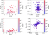 |
Fig. 2 Population A. |


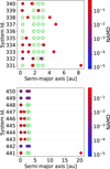 |
Fig. 3
|

3.3 Population C
Population C corresponds to the resonant counterpart of population B. Compared to population B, here we find that a larger fraction of systems remains dynamically cold over the simulated timescales (Figure 7), with only 41.6% of systems ending up dynamically hot, compared to the 72% of population B. Compared to population B, however, the fraction of disrupted systems is slightly higher (12.2% compared to 9%), which in all but one case experienced at least a close approach with the central binary. In the sampled parameter space, the majority (65.6%) of the systems do not experience catastrophic events, 27.2% of systems experience ejections or scatterings: in 11.2% of cases alone, while in 16% of cases in combination with other catastrophic events (Table 4). Normalizing the occurrence rates of catastrophic events to the frequency of dynamical hot systems, we find that 81.4% end up losing planets through catastrophic events (Table 6). In terms of the metrics  ,
,  , and ∆CoM, we find an equivalent behavior as in population B. The systems that become dynamically excited and experience planet loss end up with an increased mass concentration in the most massive planet and with an increased orbital spacing among survived planets (left panels in Figure 8). Dynamically cold systems, instead, have
  ,
,  , and ∆CoM ≃ 0 (right panels in Figure 8), meaning they preserve their initial 2:1 resonance.
 |
Fig. 4 Population B. Schematic representation of the percentage of simulated population B planetary systems (500 simulations) based on two specific properties: whether they experience at least one catastrophic event (ejection, scattering, or collision), and if they are dynamically cold or hot. The number in each box is related to the percentage of systems whose combination of parameters is specified on the x- and y-axes. In the upper right corner, we show 47% of systems that include the 9% of systems that are disrupted (see text for details). |
3.4 Population D
With population D we investigate the stability of five-planet systems in the NMS resonance (i.e., combination of 4:3 and 5:3 resonances). Compared to all the other populations, we find that all planetary systems undergo catastrophic events under the adopted priors, and the majority of systems (96.4%) end up dynamically hot (Figure 9). Nevertheless, 82.8% of planetary systems have at least one surviving planet. The most common outcome for population D planetary systems is to undergo combinations of different catastrophic events (Table 8) and lose, in the majority of cases (58%), two of their initial planets (Table 5).
All planetary systems with more than one surviving planet have  ,
,  (Figure 10), and the center of mass experiences both positive or negative shifts. All the planetary systems that end up with only one surviving planet have ∆CoM < 1 (Figure 11, the points with
  ), meaning that the surviving planet does not get scattered outward, as it happened instead with the other three populations. Depending on which one of the initial planets survived and whether it accreted other planets, its final mass is always between 1 MJ and 1.053 MJ, hence the
  metric gives similar values, and the points are overlapping in Figure 10. Illustrative examples of these scenarios are shown by system 275, 279, and 280 in Figure 12.
3.5 Dependence of the dynamical evolution on the initial multiplicity
When we divide the planetary systems based on their initial number of planets, the NAMD value of the planetary systems shows a dependence on the multiplicity (Table 7, where we report populations A, B, and C only, for which we sampled the initial number of planets). Systems initially hosting two planetary companions are more likely to remain in a stable configuration and preserve their original architectures over the simulated timescales. These systems preserve their multiplicity even when going through an excited phase, as showcased by population B in Table 7.
A large fraction of planetary systems born with more than two planets (e.g., system 222, 226, 229, and 230 in Figure 6 and system 442, 449, and 450 in Figure 3) can still experience an ordered evolution, yet the more planets initially populate a system, the more probable it is for it to go through an unstable phase, which could also disrupt it in the most catastrophic scenarios (Table 7). Under the adopted priors, the fraction of systems undergoing catastrophic events grows from 12.9% to 45.2% when going from three-planet to four-planet systems for population A, from 54.2% to 79.1% for population B, and from 51.6% to 95% for population C (Table 8). Likewise, in the case of population A, the frequency of disrupted systems grows from 0% to 0.9%, while in the case of population B and C this frequency grows from 8.1% to 18.2% and from 17.7% to 40%, respectively (Table 7).
Consistently with the explanation proposed by Turrini et al. (2020) for the NAMD-multiplicity anti-correlation in multiplanet systems around main-sequence stars, our results clearly show that, when the multiplicity of the planetary system increases so does the likelihood that the system enters an excited phase and, as a consequence, experiences ejections or scatterings and/or collisions. Reinforcing this trend, we find that all the five-planet systems, which belong to population D, experience planet loss.
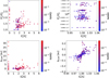 |
Fig. 5 Population B. |


4 Discussion
4.1 Observational implications of this stability study
Our results provide insight on the survival likelihood of second-generation multiplanet systems and, consequently, on the prospective gravitational-wave (GW) detection of systems possessing architectures similar to those explored in this study. Specifically, over the sampled parameter space and simulated timescales, the joint analysis of all the populations shows that 92.3% of the 2500 simulated planetary systems (i.e., 500 systems for each DWD binary) are not disrupted during their evolution. Furthermore, 39.4% of these 2500 systems preserve their initial multiplicity, while 52.9% lose at least one planet without being disrupted. Excited systems, that is, those with NAMD>1.3 × 10⁻³, are more likely to have undergone unstable phases and to have experienced catastrophic events, which in the majority of cases are ejections (Table 4; Figures 1, 4, 7, and 9 for population A, B, C, and D, respectively). When we combine the four populations and analyze them as a single one, we see that in 15.9% of cases the planetary systems experienced scatterings or ejections, while in 17.8% of cases the systems underwent multiple catastrophic events. In these extreme scenarios, where multiple catastrophic events take place, the planetary systems are generally disrupted. Disruptions, however, affect 0.2% of the systems in population A, 9% of the systems in population B, 12.2% of systems in population C, and 17.2% of systems in population D, corresponding to 7.7% of the total 2500 simulated systems. The reason why disruptions are more frequent in population B and C rather than population A is that population B and C have more massive planets orbiting around a more massive binary, resulting in stronger gravitational perturbations between the bodies in the systems. The higher disruption fraction in population D instead reflects the initial higher multiplicity, which is five for all these simulated systems, and the effects of the perturbations are enhanced by the more packed architecture.
Concerning the difference between initial nonresonant architectures and resonant ones, we can compare population B with population C, which employ the same binary system and sample the same range of planet masses, with the difference that in population C the planets are initially in a 2:1 resonance. Under the adopted priors, more orbital architectures remain dynamically cold when they are in resonance (Figures 4 and 7). When dividing the systems based on their initial multiplicity we also see that the fraction of stable two- and three-planet systems is higher when such systems are in resonance (Table 6). In both populations B and C, however, the majority of three- and four-planet systems experience catastrophic events, and actually the fraction of four-planet systems that are disrupted is larger when these systems are in resonance. Moreover, in population D, where we employ five-planet systems that are initially in the NMS resonance, we find that the majority (96.4%) of systems end up dynamically hot and all systems lose at least one planet, breaking the resonant chain (Tables 4 and 5).
The resonant and the nonresonant scenarios show that NAMD and the catastrophic events that a system experiences are linked to its initial multiplicity. Systems with higher multiplicity are more likely to undergo unstable phases after being excited (Tables 7 and 8). Systems with an initial planet multiplicity of two never experience catastrophic events, even the 26.3% of population B and the 7% of population C two-planet systems that end up in excited architectures. Among all simulated two-planet systems, this scenario happened 7% of times. Furthermore, 30.5% of planetary systems with initially three, four, or five planets end up with two surviving ones, increasing our initial two-planet population by 122% and creating a degeneracy in knowing the past of potentially observed two-planet systems.
To this regard, in Figure 13 we show the NAMD as a function of the final number of planets, Nf, represented as circles and color-coded by the number of lost planets. The gray squares indicate the mean NAMD value for each Nf bin. We find an anti-correlation between the NAMD and the final system multiplicity, in agreement with the results of Turrini et al. (2020).
Furthermore, as proposed also by Turrini et al. (2020) for main-sequence stars, our results suggest that we can assess the likelihood that such observed two-planet systems had higher primordial multiplicity by quantifying their NAMD values after we characterize the orbits of their planets. If the NAMD > 1.3 × 10⁻³, that is, the system is more dynamically excited than the Solar System, it is plausible that the system itself was originally more populated since in the majority of cases the two-planet systems that do not experience catastrophic events remain dynamically colder than this threshold value. This insight opens up the possibility to infer the loss of planets within second-generation systems hosting giant planets. As the results of Ledda et al. (2023) highlight that giant planets can form only over limited temporal intervals in second-generation disks, constraining how frequent these giant planets are can provide independent constraints on the timescale and efficiency of the planet formation process. It must be pointed out, however, that this observational outlook does not account for the possible presence within the system of first-generation planets that survived the evolution of the inner binary (Columba et al. 2023). Disentangling this possible source of degeneracy will require dedicated studies of planet formation within second-generation disks in the presence of a wide orbit planet (Columba et al. 2023), and of the orbital stability of the newly formed systems, which are beyond the scope of this paper.
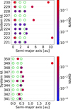 |
Fig. 6
|

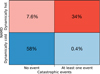 |
Fig. 7 Population C. Schematic representation of the percentage of simulated planetary systems (500 simulations) based on two specific properties: whether they experience at least one catastrophic event (ejection, scattering, or collision), and if they are dynamically cold or hot. The number in each box is related to the percentage of systems whose combination of parameters is specified on the x- and y-axes. In the upper right corner, we show 34% of systems that include the 12.2% of systems that are disrupted (see text for details). |
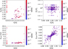 |
Fig. 8 Population C. |


 |
Fig. 9 Population D. Schematic representation of the percentage of simulated planetary systems (500 simulations) based on two specific properties: whether they experience at least one catastrophic event (ejection, scattering, or collision), and if they are dynamically cold or hot. The number in each box is related to the percentage of systems whose combination of parameters is specified on the x- and y-axes. In the upper right corner, we show 96.4% of systems that include the 17.2% of systems that are disrupted (see text for details). |
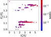 |
Fig. 10 Population D. |


Percentage of population A, B, and C planetary systems with the NAMD value in a given range.
Percentage of the population A, B, and C planetary systems that experienced catastrophic events.
4.2 The LISA framework
In the context of the future ESA-LISA space mission, we now focus on  and
and  , as they belong to the LISA DWD synthetic population. This means that, when such systems are placed within the context of the Milky Way’s history, the frequency fGW of their GW falls within the LISA band (Korol et al. 2017, 2019; Amaro-Seoane et al. 2023a). For such, any substellar object orbiting these binaries might have the potential to be detected, provided that the signal-to-noise of the binary S DWD is larger than around 10 (Danielski et al. 2019, their Figure A.1) and that the orbital period and mass of the companion are optimal for causing a detectable modulation of the GW signal. We note that the considerations we draw in the following, concerning the possible GW detection of our simulated systems, are purely qualitative and model dependent, since detailed assessment of their detectability is beyond the scope of this article. Dedicated studies would need to be performed to test whether LISA can hear the systems here studied. Multiplanet detection with LISA is a topic that has yet to be investigated: the presence of more than one planet would change the gravitational perturbation on the binary, and consequently also the final waveform compared to what presented in Danielski et al. (2019) and Katz et al. (2022), based on a single-planet approach.
For what it concerns those systems that end up with only one substellar object, most of the bodies (i.e., a total of 121 planets and 28 brown dwarfs, Figure 14) have masses Mp greater than 4 MJ and a period shorter than half the observing time of the nominal mission of LISA (4 years, assuming 100% duty cycle). Following the results by Katz et al. (2022) these single-planet systems have the potential to be detected, pending their distance, sky-location, and polarization angle (Robson et al. 2018). Overall, the GW signal-to-noise ratio of a DWD is determined by these parameters, together with the binary’s chirp mass, orbital period, and eccentricity, if any. Since the detection of Magrathea planets relies on the perturbation of the binary’s center of mass, their detectability primarily depends on the planetary mass and orbital separation. We refer the reader to Danielski et al. (2019), their Appendix A, for a detailed study of the parameter space covered by Magrathea planets and brown dwarfs.
Concerning those systems with more than one planet, we can assess as a first approximation the detectability of each planetary system around  and
and  , by measuring the GW frequency shift amplitude produced by the planets in their systems. Following the syntax of Danielski et al. (2019), the motion of the DWD around the center of mass of a three body system modulates the GW frequency through the Doppler effect where the resulting frequency observed by LISA is
 (12)
(12)
v∥ = −K cos φ(t) is the line-of-sight velocity of the DWD with respect to the common center of mass, fGW = 2 · forb is the GW frequency in the reference frame at rest with respect to the DWD center of mass, and forb is the orbital frequency of the binary (Maggiore 2008; Postnov & Yungelson 2014). The parameter c is the speed of light, φ(t) is the orbital phase (see Danielski et al. 2019, their Eq. (5)), and K is the amplitude of the radial velocity signal caused by the presence of the third object orbiting the binary and it is defined as
 (13)
where P, M, and i are the third body period, mass, and inclination, respectively. Mbin is the DWD total mass, and G the gravitational constant. Given that the average cos φ(t) ∼ 1 the GW frequency shift amplitude for a system with one planet can be approximated from Eq. (12) as
(13)
where P, M, and i are the third body period, mass, and inclination, respectively. Mbin is the DWD total mass, and G the gravitational constant. Given that the average cos φ(t) ∼ 1 the GW frequency shift amplitude for a system with one planet can be approximated from Eq. (12) as
 (14)
(14)
Yet, in the event of a multiplanet system with N planets, assuming that their orbital angular momentum vectors are isotropically distributed, that is, the average of sin i = π/4, we can then approximate the global shift as
 (15)
(15)
For all systems we analyzed, this shift is smaller than LISA frequency resolution of ∼7.92 × 10⁻⁹ Hz for a 4-year mission. The majority of systems are also below the frequency resolution of 3.96 × 10⁻⁹ Hz (8-year mission), except for a handful of population C systems (bottom left panel in Figure 15).
The GW frequency emitted by the  and
and  binaries ( fGW = 0.36 mHz, 0.32 mHz respectively) lies within the LISA band (i.e., 0.1 mHz–1 Hz, Amaro-Seoane et al. 2023b), meaning that their detection is possible, provided that the distance to the binaries is favorable. However, the GW shift induced by the planets in each system would be too small to be detected by LISA in the majority of the cases. The conclusions we can draw based on these results are two: (i) a specific waveform study, such as the one by Katz et al. (2022), done for a single-planet system case, is needed to definitively test whether each system is realistically detectable; (ii) the shift was computed using the binary parameters right after the second common envelope phase. Yet, the binary will shrink over time, shortening the orbital period and hence increasing the orbital frequency. An increase in the orbital frequency would allow for a higher probability of detection of a third body perturbing the DWD (Danielski et al. 2019). For instance, in the case of a two-planet system (like system 219 from population B, characterized by ∆f = 1.50 × 10⁻⁹ Hz), the binary period should shrink by a factor of six or three to make the frequency shift amplitude caused by the planets detectable for an 8- or 4-year mission, respectively. We note that we studied the stability of the systems formed around
  and
and  over 10 Myr after the formation of the DWD itself. On this timescale, the period of the binary itself would have shortened by only ∼2.3 minutes and ∼1 minute for
  and
and  , respectively3. Each DWD is expected to merge in 150 Myr and 430 Myr (Table 9).
Another way to test the possibility of planetary system detection by LISA is to check the acceleration of the CoM. When the acceleration is non negligible, it will leave an imprint on the GW signal; an apparent acceleration along the line of sight will cause each DWD to exhibit an apparent GW frequency chirp (e.g., Xuan et al. 2023; Ebadi et al. 2024). To qualitatively illustrate this point, we selected two systems from population B (system 126 and 235, Table 9) with the largest CoM shift, and we measured the average acceleration over a 8 years timescale (i.e., the duration of the LISA extended mission). The acceleration increases for both systems as a consequence of planetary ejections from the system (see Figure 16 for system 235; the CoM acceleration of system 126 reaches a similar average acceleration but earlier in time). The average acceleration was aCoM ∼ 0.4 au/yr2 for both systems, followed by an average acceleration of 0.9 au/yr2 after ejections happened. Furthermore, the dispersion of the acceleration also increased, passing from ∆aCoM = 0.6 au/yr2 to ∆aCoM = 1.0 au/yr2. In terms of timescales, ejections began at 2.00×10³ yr and 9.22×10⁵ yr, and occurred over a timeframe of 1.80×10⁴ yr and 1.99×10⁵ yr for system 126 and 235, respectively. At the time of writing the minimum aCoM for a system to be detected by LISA has not been defined yet. Future studies focusing on the planetary induced accelerations are to be developed, and will be able to address whether the acceleration of the CoM of the systems presented here is sufficient or not to improve the planetary detection rates of LISA.
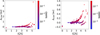 |
Fig. 11 Population D. ∆CoM as a function of |

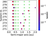 |
Fig. 12
|

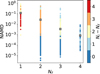 |
Fig. 13 Final multiplicity vs. NAMD for all the planetary systems we considered (colored circles) and for the average values of each multiplicity bin (gray squares). The color bar indicates the number of lost planets for each system. |
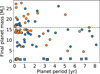 |
Fig. 14 Population B (blue circles), population A (blue squares), population C (orange circles), and population D (orange squares) systems. Final planet mass vs. final planet period. The dashed red line at Mp = 16 MJ represents the threshold that separates planets from brown dwarfs as discussed in Spiegel et al. (2011). We end up with brown dwarfs because some planets undergo collisional merge, and the resulting total planet mass is greater than 16 MJ. We note that some points are overlapping with each other, especially the ones relative to population D. |
Shortest and longest times needed for  and
and  systems to form giant planets and to reach a stable orbital configuration, and time needed for the stars in the binary to merge.
4.3 Caveats and model limitations
Before drawing our conclusions, we want to emphasize that, due to the computational cost of the simulations, our integration times probe the early phases of dynamical evolution of DWD systems, whose lifetime is significantly longer than what modeled in this study. Furthermore, we stress that stability studies are in general sensitive to the assumed initial conditions, and our results are therefore valid within the limits of the assumed priors and sampled parameter space. In terms of physical assumptions, we note that our simulations do not account for general relativity effects, tidal interaction, binary period shrinkage, secular resonances, and radiation forces, as the addition of such physical processes is beyond of the scope of the current work. Finally, the discussion on the prospective detectability of similar systems with LISA should be regarded as illustrative, since it relies on possible synthetic architectures of second-generation multiplanet systems.
 |
Fig. 15 Population B (top left), population A (top right), population C (bottom left), and population D (bottom right) systems. Global frequency shift ∆ f computed with Eq. (15). |
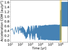 |
Fig. 16 Acceleration of the planetary center of mass vs. time for system 235, which experienced one of the largest |∆CoM|. The yellow shaded region indicates when ejections took place in the simulation. |
5 Conclusions
This work has been developed within the framework of the planetary detection science case of the LISA mission, which will greatly advance our understanding of the Universe via GW astronomy. The mission will shed light on a variety of unanswered questions, and one of these is whether planets can form and/or survive around binary systems in which both stars evolved into white dwarfs. Although circumbinary planets have been found around evolved systems, to date, none of these is orbiting a DWD. The most probable reason for the lack of detection is the selection bias in the observations that arises from the faintness of the stellar hosts. Kostov et al. (2016), and more recently, Columba et al. (2023), proved that planets can survive the catastrophic events that occur during the evolution of a binary system. At the same time, Ledda et al. (2023) showed that a second generation of giant planets can form from the ejected material that remains bound to the binary. The research work we performed takes us a step ahead. We investigated the orbital evolution of giant planets around DWDs with N-body simulations to determine whether the planets that formed within a second-generation circumbinary disk are dynamically stable and can survive for us to observe them, or if they are destabilized.
Our study showed that when giant planets form around DWDs, these planets can survive over multiple million years after disk dispersal (see Tables 4, 5, and 6 for a summary of the results). In the sampled parameter space, we found that more massive binaries hosting more massive planets, our populations B and C, are more likely to experience unstable phases and catastrophic events compared to the less massive counterpart, our population A (Figures 1, 4, and 7). The most common catastrophic event experienced by our systems is the scattering or ejection of planets. In the most extreme scenarios, in which multiple catastrophic events occur, and especially when planets experience close encounters with the binary, the planetary systems are disrupted. Of all the 2500 simulated planetary systems, 7.7% are disrupted, while 92.3% have at least one planet that survives the dynamical evolution. Dynamically hot systems, which are the product of chaotic evolution, always evolve toward less compact architectures, and the most massive planet contains larger fractions of the final planetary mass. In addition, dynamically hot systems can experience strong shifts in the center of mass, even up to ∼30 au (Figure 11 and bottom panels of Figures 2, 5, and 8). In contrast, dynamically cold systems, which experience an ordered evolution, preserve their initial orbital architecture and loose no mass.
In the comparison of the nonresonant with the initially resonant configurations, our results indicate that planetary systems born in resonance tend to preserve dynamically cold configurations over time. Resonant setups, in contrast, enhance the stability of low-multiplicity systems overall (two or three planets), and higher-multiplicity resonant systems instead prove more prone to instability and planet loss. In particular, nearly all four-planet systems and all five-planet systems that started in resonant chains ultimately broke the resonance by losing at least one planet.
Considering all four populations as a whole, we found that systems with a higher initial multiplicity are more likely to undergo unstable phases, in which ejections and collisions can take place. We also found that the final planetary multiplicity is anticorrelated with their dynamical excitation (recorded by their NAMD value), which agrees with the findings of Turrini et al. (2020) for observed multiplanetary systems (Figure 13). Two-planet systems remain dynamically cold in the majority of cases and preserve all their original planets. On the other hand, the five-planet population proved highly prone to disruption, while the four-planet population decreased by 56.1% and the three-planet population decreased by 22.5%. These decreases led to an increase (122%) in the two-planet population and created a new single-planet population (7.1% of all the systems). Our findings are consistent with the interpretation of Turrini et al. (2020), who suggested that low-multiplicity systems are often the outcome of dynamical instabilities that removed some of their primordial planets.
Furthermore, most of the single-planet systems, given their planet mass and period, might be detected by LISA, provided that the GW signal-to-noise ratio of the system based on their distance, sky location, polarization, and inclination is high enough for the systems to be detected. We provided a formula (Eq. (15)) for the GW detection of multiplanet systems to approximate the global frequency shift that the planets would exert on the GW produced by the DWD. For the systems we studied, this frequency shift is weaker for most systems than the frequency resolution of LISA, which indicates that these multiplanet systems are probably not detectable by LISA. For a handful of resonant systems (population C), the frequency shift caused by planets in the same system is strong enough to be detected within 8 years of LISA observations. Nevertheless, specific Bayesian studies that account for a multibody waveform and the orbital shrinking of the binary, should be performed to confirm or refute the detectability (e.g., Katz et al. 2022 for single-planet systems). It is important to approach these detectability considerations as illustrative of the potential capabilities of LISA for planetary detection and not as predictions, in particular, because they are based on synthetic architectures. Finally, we studied the acceleration of the center of mass of two systems that presented the strongest inward and outward CoM shift during their evolution. An acceleration of the CoM can leave an imprint on the GW signal that can improve the system detectability. No acceleration threshold value has been studied for the LISA planetary system case so far, but the average acceleration of our two systems is 0.9 au/yr2. If the LISA threshold value were proved to be lower than 0.9 au/yr2, Magrathea planets would have one more chance to be found by GW astronomy.
Acknowledgements
We thank N. Tamanini for the helpful discussions. This work has been developed within the framework of the “LISA Triple and CBPs” project of the LISA Astrophysical WG of the ESA LISA mission Consortium. A.N. acknowledges support from the Swiss National Science Foundation (SNSF) under grant PZ00P2_208945. D.T. and D.P. acknowledge support by the Fondazione ICSC, Spoke 3 “Astrophysics and Cosmos Observations”, National Recovery and Resilience Plan (Piano Nazionale di Ripresa e Resilienza, PNRR) Project ID CN_00000013 “Italian Research Center on High-Performance Computing, Big Data and Quantum Computing” funded by MUR Missione 4 Componente 2 Investimento 1.4: Potenziamento strutture di ricerca e creazione di “campioni nazionali di R&S (M4C2-19)” – Next Generation EU (NGEU). D.T. and D.P. also acknowledge support from the ASI-INAF grant no. 2021-5-HH.0 plus addenda nos. 2021-5-HH.1-2022 and 2021-5-HH.2-2024, the COST Action CA22133 PLANETS. D.T. also acknowledges the European Research Council via the Horizon 2020 Framework Programme ERC Synergy “ECO-GAL” Project GA-855130. C.D. acknowledges financial support from the grant RYC2023-044903-I funded by MCIU/AEI/10.13039/501100011033 and by the ESF+, and from the INAF initiative “IAF Astronomy Fellowships in Italy”, grant name GExoLife.
References
- Adelbert, S., Penzlin, A. B. T., Schäfer, C. M., et al. 2023, A&A, 680, A29 [NASA ADS] [CrossRef] [EDP Sciences] [Google Scholar]
- Amaro-Seoane, P., Audley, H., Babak, S., et al. 2017, arXiv e-prints [arXiv:1702.00786] [Google Scholar]
- Amaro-Seoane, P., Andrews, J., Arca Sedda, M., et al. 2023a, Liv. Rev. Relat., 26, 2 [NASA ADS] [CrossRef] [Google Scholar]
- Amaro-Seoane, P., Andrews, J., Arca Sedda, M., et al. 2023b, Liv. Rev. Relat., 26, 2 [NASA ADS] [CrossRef] [Google Scholar]
- Armstrong, D. J., Osborn, H. P., Brown, D. J. A., et al. 2014, MNRAS, 444, 1873 [CrossRef] [Google Scholar]
- Baycroft, T. A., Santerne, A., Triaud, A. H. M. J., et al. 2025, MNRAS, 541, 2801 [Google Scholar]
- Beuermann, K., Hessman, F. V., Dreizler, S., et al. 2010, A&A, 521, L60 [NASA ADS] [CrossRef] [EDP Sciences] [Google Scholar]
- Chambers, J. E. 1999, MNRAS, 304, 793 [Google Scholar]
- Chambers, J. E. 2001, Icarus, 152, 205 [Google Scholar]
- Chambers, J. E., Wetherill, G. W., & Boss, A. P. 1996, Icarus, 119, 261 [Google Scholar]
- Chambers, J. E., Quintana, E. V., Duncan, M. J., & Lissauer, J. J. 2002, AJ, 123, 2884 [NASA ADS] [CrossRef] [Google Scholar]
- Columba, G., Danielski, C., Dorozsmai, A., Toonen, S., & Lopez Puertas, M. 2023, A&A, 675, A156 [NASA ADS] [CrossRef] [EDP Sciences] [Google Scholar]
- Danielski, C., & Tamanini, N. 2020, Int. J. Mod. Phys. D, 29, 2043007 [NASA ADS] [CrossRef] [Google Scholar]
- Danielski, C., Korol, V., Tamanini, N., & Rossi, E. M. 2019, A&A, 632, A113 [NASA ADS] [CrossRef] [EDP Sciences] [Google Scholar]
- Doyle, L. R., Carter, J. A., Fabrycky, D. C., et al. 2011, Science, 333, 1602 [NASA ADS] [CrossRef] [Google Scholar]
- Ebadi, R., Strokov, V., Tanin, E. H., Berti, E., & Walsworth, R. L. 2024, arXiv e-prints [arXiv:2405.13109] [Google Scholar]
- Gajdoš, P., & Vaňko, M. 2023, MNRAS, 518, 2068 [Google Scholar]
- Gallardo Cava, I., Gómez-Garrido, M., Bujarrabal, V., et al. 2021, A&A, 648, A93 [NASA ADS] [CrossRef] [EDP Sciences] [Google Scholar]
- Georgakarakos, N., Eggl, S., Ali-Dib, M., & Dobbs-Dixon, I. 2024, AJ, 168, 224 [Google Scholar]
- Gong, Y.-X., & Ji, J. 2017, AJ, 154, 179 [Google Scholar]
- Holman, M. J., & Wiegert, P. A. 1999, AJ, 117, 621 [Google Scholar]
- Hu, Y.-M. 2025, in Proceedings of the 7th International Workshop on the Tian-Qin Science Mission, 25–26 April 2024, Hong Kong SAR, China, eds. J. Luo, V. Milyukov, Z.-B. Zhou, H.-C. Yeh, & J. Mei (Singapore: Springer Nature Singapore), 25 [Google Scholar]
- Huang, S.-J., Hu, Y.-M., Korol, V., et al. 2020, Phys. Rev. D, 102, 063021 [NASA ADS] [CrossRef] [Google Scholar]
- Izidoro, A., Ogihara, M., Raymond, S. N., et al. 2017, MNRAS, 470, 1750 [Google Scholar]
- Kang, Y., Liu, C., & Shao, L. 2021, AJ, 162, 247 [Google Scholar]
- Kashi, A., & Soker, N. 2011, MNRAS, 417, 1466 [NASA ADS] [CrossRef] [Google Scholar]
- Katz, M. L., Danielski, C., Karnesis, N., et al. 2022, MNRAS, 517, 697 [NASA ADS] [CrossRef] [Google Scholar]
- Kluska, J., Van Winckel, H., Coppée, Q., et al. 2022, A&A, 658, A36 [NASA ADS] [CrossRef] [EDP Sciences] [Google Scholar]
- Korol, V., Rossi, E. M., Groot, P. J., et al. 2017, MNRAS, 470, 1894 [NASA ADS] [CrossRef] [Google Scholar]
- Korol, V., Rossi, E. M., & Barausse, E. 2019, MNRAS, 483, 5518 [NASA ADS] [CrossRef] [Google Scholar]
- Kostov, V. B., Moore, K., Tamayo, D., Jayawardhana, R., & Rinehart, S. A. 2016, ApJ, 832, 183 [NASA ADS] [CrossRef] [Google Scholar]
- Kostov, V. B., Orosz, J. A., Feinstein, A. D., et al. 2020, AJ, 159, 253 [Google Scholar]
- Kostov, V. B., Powell, B. P., Orosz, J. A., et al. 2021, AJ, 162, 234 [NASA ADS] [CrossRef] [Google Scholar]
- Laskar, J., & Petit, A. C. 2017, A&A, 605, A72 [NASA ADS] [CrossRef] [EDP Sciences] [Google Scholar]
- Ledda, S., Danielski, C., & Turrini, D. 2023, A&A, 675, A184 [NASA ADS] [CrossRef] [EDP Sciences] [Google Scholar]
- Limbach, M. A., & Turner, E. L. 2015, PNAS, 112, 20 [NASA ADS] [CrossRef] [Google Scholar]
- Lipunov, V. M., & Postnov, K. A. 1988, Ap & SS, 145, 1 [Google Scholar]
- Lissauer, J. J., & de Pater, I. 2019, Fundamental Planetary Science: Physics, Chemistry and Habitability (Cambridge University Press) [Google Scholar]
- Maggiore, M. 2008, Gravitational Waves, 2 (Oxford University Press) [Google Scholar]
- Martin, D. V. 2018, in Handbook of Exoplanets, eds. H. J. Deeg, & J. A. Belmonte, 156 [Google Scholar]
- Martin, D. V., Triaud, A. H. M. J., Udry, S., et al. 2019, A&A, 624, A68 [NASA ADS] [CrossRef] [EDP Sciences] [Google Scholar]
- Marzari, F., & Thebault, P. 2019, Galaxies, 7, 84 [NASA ADS] [CrossRef] [Google Scholar]
- Nelemans, G., Yungelson, L. R., Portegies Zwart, S. F., & Verbunt, F. 2001, A&A, 365, 491 [NASA ADS] [CrossRef] [EDP Sciences] [Google Scholar]
- Nesvorný, D., & Morbidelli, A. 2012, AJ, 144, 117 [Google Scholar]
- Obertas, A., Van Laerhoven, C., & Tamayo, D. 2017, Icarus, 293, 52 [NASA ADS] [CrossRef] [Google Scholar]
- Perets, H. B. 2010, arXiv e-prints [arXiv:1001.0581] [Google Scholar]
- Postnov, K. A., & Yungelson, L. R. 2014, Liv. Rev. Relat., 17, 3 [NASA ADS] [CrossRef] [Google Scholar]
- Potter, S. B., Romero-Colmenero, E., Ramsay, G., et al. 2011, MNRAS, 416, 2202 [NASA ADS] [CrossRef] [Google Scholar]
- Przyłuski, R., Rickman, H., Wajer, P., et al. 2025, Universe, 11, 240 [Google Scholar]
- Quarles, B., Satyal, S., Kostov, V., Kaib, N., & Haghighipour, N. 2018, ApJ, 856, 150 [NASA ADS] [CrossRef] [Google Scholar]
- Rickman, H., Wajer, P., Przyłuski, R., et al. 2023, MNRAS, 520, 637 [NASA ADS] [CrossRef] [Google Scholar]
- Robson, T., Cornish, N. J., Tamanini, N., & Toonen, S. 2018, Phys. Rev. D, 98, 064012 [NASA ADS] [CrossRef] [Google Scholar]
- Seto, N. 2008, ApJ, 677, L55 [Google Scholar]
- Socia, Q. J., Welsh, W. F., Orosz, J. A., et al. 2020, AJ, 159, 94 [Google Scholar]
- Spiegel, D. S., Burrows, A., & Milsom, J. A. 2011, ApJ, 727, 57 [Google Scholar]
- Standing, M. R., Sairam, L., Martin, D. V., et al. 2023, Nat. Astron., 7, 702 [NASA ADS] [CrossRef] [Google Scholar]
- Tamanini, N., & Danielski, C. 2019, Nat. Astron., 3, 858 [NASA ADS] [CrossRef] [Google Scholar]
- Triaud, A. H. M. J., Standing, M. R., Heidari, N., et al. 2022, MNRAS, 511, 3561 [NASA ADS] [CrossRef] [Google Scholar]
- Turrini, D., Marzari, F., Polychroni, D., & Testi, L. 2019, ApJ, 877, 50 [NASA ADS] [CrossRef] [Google Scholar]
- Turrini, D., Zinzi, A., & Belinchon, J. A. 2020, A&A, 636, A53 [NASA ADS] [CrossRef] [EDP Sciences] [Google Scholar]
- Turrini, D., Schisano, E., Fonte, S., et al. 2021, ApJ, 909, 40 [Google Scholar]
- Turrini, D., Codella, C., Danielski, C., et al. 2022, Exp. Astron., 53, 225 [CrossRef] [Google Scholar]
- Tutukov, A. V., & Yungelson, L. R. 1979, Acta Astron., 29, 665 [NASA ADS] [Google Scholar]
- Van Winckel, H. 2018, arXiv e-prints [arXiv:1809.00871] [Google Scholar]
- Verrier, P. 2008, The Dynamics of Planets in Multistellar Systems, PhD thesis, Institute of Astronomy University of Cambridge Wisdom, J., & Holman, M. 1991, AJ, 102, 1528 [Google Scholar]
- Xuan, Z., Naoz, S., & Chen, X. 2023, Phys. Rev. D, 107, 043009 [Google Scholar]
- Zinzi, A., & Turrini, D. 2017, A&A, 605, L4 [NASA ADS] [CrossRef] [EDP Sciences] [Google Scholar]
A more appropriate denomination of disks and planets that form in the last stage of the binary evolution would be third-generation disks.
An orbital mean motion resonance between two planets occurs when their orbital periods are nearly commensurate, that is, they can be expressed as a ratio of two small integers (Lissauer & de Pater 2019), that cause chaotic dynamical regions that surround the inner binary (see Marzari & Thebault 2019 for a review on the topic).
This example is meant only to provide an order of magnitude of the binary frequency change. It is computed based on Eq. (9) of Danielski et al. (2019) and it is meant for a DWD alone, excluding the dynamical contribution of planetary companions.
All Tables
Stellar masses, periods, binary separations, and critical semimajor axis of the three analyzed DWDs.
Initial planet mass and semimajor axes for the resonant five- planet systems orbiting the binary.
Percentage of population A, B, C, and D planetary systems that experienced catastrophic events.
Percentage of population A, B, C, and D planetary systems that loose none, one, two, three, four, or five planets.
Percentage of systems that experienced catastrophic events over the subsample of excited population A, B, C, and D systems (i.e., NAMD>1.3×10⁻³).
Percentage of population A, B, and C planetary systems with the NAMD value in a given range.
Percentage of the population A, B, and C planetary systems that experienced catastrophic events.
Shortest and longest times needed for and systems to form giant planets and to reach a stable orbital configuration, and time needed for the stars in the binary to merge.
All Figures
|
Fig. 1 Population A. Schematic representation of the percentage of simulated planetary systems (1000 simulations in total for DWD2 and DWD∗4) based on two specific properties: whether they experience at least one catastrophic event (ejection, scattering, or collision), and whether they are dynamically cold or hot. The number in each box is related to the percentage of systems whose combination of parameters is specified on the x- and y-axes. In the upper right corner, we show 14.1% of systems that include the 0.2% of systems that are disrupted (see text for details). |
| In the text | |
|
Fig. 2 Population A. |
| In the text | |
|
Fig. 3
|
| In the text | |
|
Fig. 4 Population B. Schematic representation of the percentage of simulated population B planetary systems (500 simulations) based on two specific properties: whether they experience at least one catastrophic event (ejection, scattering, or collision), and if they are dynamically cold or hot. The number in each box is related to the percentage of systems whose combination of parameters is specified on the x- and y-axes. In the upper right corner, we show 47% of systems that include the 9% of systems that are disrupted (see text for details). |
| In the text | |
|
Fig. 5 Population B. |
| In the text | |
|
Fig. 6
|
| In the text | |
|
Fig. 7 Population C. Schematic representation of the percentage of simulated planetary systems (500 simulations) based on two specific properties: whether they experience at least one catastrophic event (ejection, scattering, or collision), and if they are dynamically cold or hot. The number in each box is related to the percentage of systems whose combination of parameters is specified on the x- and y-axes. In the upper right corner, we show 34% of systems that include the 12.2% of systems that are disrupted (see text for details). |
| In the text | |
|
Fig. 8 Population C. |
| In the text | |
|
Fig. 9 Population D. Schematic representation of the percentage of simulated planetary systems (500 simulations) based on two specific properties: whether they experience at least one catastrophic event (ejection, scattering, or collision), and if they are dynamically cold or hot. The number in each box is related to the percentage of systems whose combination of parameters is specified on the x- and y-axes. In the upper right corner, we show 96.4% of systems that include the 17.2% of systems that are disrupted (see text for details). |
| In the text | |
|
Fig. 10 Population D. |
| In the text | |
|
Fig. 11 Population D. ∆CoM as a function of |
| In the text | |
|
Fig. 12
|
| In the text | |
|
Fig. 13 Final multiplicity vs. NAMD for all the planetary systems we considered (colored circles) and for the average values of each multiplicity bin (gray squares). The color bar indicates the number of lost planets for each system. |
| In the text | |
|
Fig. 14 Population B (blue circles), population A (blue squares), population C (orange circles), and population D (orange squares) systems. Final planet mass vs. final planet period. The dashed red line at Mp = 16 MJ represents the threshold that separates planets from brown dwarfs as discussed in Spiegel et al. (2011). We end up with brown dwarfs because some planets undergo collisional merge, and the resulting total planet mass is greater than 16 MJ. We note that some points are overlapping with each other, especially the ones relative to population D. |
| In the text | |
|
Fig. 15 Population B (top left), population A (top right), population C (bottom left), and population D (bottom right) systems. Global frequency shift ∆ f computed with Eq. (15). |
| In the text | |
|
Fig. 16 Acceleration of the planetary center of mass vs. time for system 235, which experienced one of the largest |∆CoM|. The yellow shaded region indicates when ejections took place in the simulation. |
| In the text | |
Current usage metrics show cumulative count of Article Views (full-text article views including HTML views, PDF and ePub downloads, according to the available data) and Abstracts Views on Vision4Press platform.
Data correspond to usage on the plateform after 2015. The current usage metrics is available 48-96 hours after online publication and is updated daily on week days.
Initial download of the metrics may take a while.