| Issue |
A&A
Volume 706, February 2026
|
|
|---|---|---|
| Article Number | A25 | |
| Number of page(s) | 13 | |
| Section | Stellar structure and evolution | |
| DOI | https://doi.org/10.1051/0004-6361/202555431 | |
| Published online | 27 January 2026 | |
CTAO LST–1 observations of magnetar SGR 1935+2154: Deep limits on sub-second bursts and persistent tera-electronvolt emission
1
Department of Physics, Tokai University, 4-1-1 Kita-Kaname Hiratsuka Kanagawa 259-1292, Japan
2
Institute for Cosmic Ray Research, University of Tokyo, 5-1-5 Kashiwa-no-ha Kashiwa Chiba 277-8582, Japan
3
INFN and Università degli Studi di Siena, Dipartimento di Scienze Fisiche, della Terra e dell’Ambiente (DSFTA), Sezione di Fisica Via Roma 56 53100 Siena, Italy
4
Université Paris-Saclay, Université Paris Cité, CEA, CNRS, AIM F-91191 Gif-sur-Yvette Cedex, France
5
FSLAC IRL 2009, CNRS/IAC La Laguna Tenerife, Spain
6
Departament de Física Quàntica i Astrofísica, Institut de Ciències del Cosmos, Universitat de Barcelona, IEEC-UB, Martí i Franquès 1 08028 Barcelona, Spain
7
Instituto de Astrofísica de Andalucía-CSIC Glorieta de la Astronomía s/n 18008 Granada, Spain
8
Department of Astronomy, University of Geneva Chemin d’Ecogia 16 CH-1290 Versoix, Switzerland
9
INFN Sezione di Napoli, Via Cintia ed. G 80126 Napoli, Italy
10
INAF – Osservatorio Astronomico di Roma Via di Frascati 33 00040 Monteporzio Catone, Italy
11
Max-Planck-Institut für Physik Boltzmannstraße 8 85748 Garching bei München, Germany
12
INFN Sezione di Padova and Università degli Studi di Padova Via Marzolo 8 35131 Padova, Italy
13
Instituto de Astrofísica de Canarias and Departamento de Astrofísica, Universidad de La Laguna, C. Vía Láctea s/n 38205 La Laguna Santa Cruz de Tenerife, Spain
14
Univ. Savoie Mont Blanc, CNRS, Laboratoire d’Annecy de Physique des Particules – IN2P3 74000 Annecy, France
15
Universität Hamburg, Institut für Experimentalphysik Luruper Chaussee 149 22761 Hamburg, Germany
16
Graduate School of Science, University of Tokyo, 7-3-1 Hongo Bunkyo-ku Tokyo 113-0033, Japan
17
IPARCOS-UCM, Instituto de Física de Partículas y del Cosmos, and EMFTEL Department, Universidad Complutense de Madrid, Plaza de Ciencias 1. Ciudad Universitaria 28040 Madrid, Spain
18
Faculty of Science and Technology, Universidad del Azuay Cuenca, Ecuador
19
Centro Brasileiro de Pesquisas Físicas Rua Xavier Sigaud 150 RJ 22290-180 Rio de Janeiro, Brazil
20
CIEMAT Avda. Complutense 40 28040 Madrid, Spain
21
University of Geneva – Département de physique nucléaire et corpusculaire 24 Quai Ernest Ansernet 1211 Genève 4, Switzerland
22
INFN Sezione di Bari and Politecnico di Bari Via Orabona 4 70124 Bari, Italy
23
Institut de Fisica d’Altes Energies (IFAE), The Barcelona Institute of Science and Technology, Campus UAB 08193 Bellaterra (Barcelona), Spain
24
INAF – Osservatorio Astronomico di Brera Via Brera 28 20121 Milano, Italy
25
Faculty of Physics and Applied Informatics, University of Lodz ul. Pomorska 149-153 90-236 Lodz, Poland
26
INAF – Osservatorio di Astrofisica e Scienza dello spazio di Bologna Via Piero Gobetti 93/3 40129 Bologna, Italy
27
Dipartimento di Fisica e Astronomia (DIFA) Augusto Righi, Università di Bologna Via Gobetti 93/2 I-40129 Bologna, Italy
28
Lamarr Institute for Machine Learning and Artificial Intelligence 44227 Dortmund, Germany
29
INFN Sezione di Trieste and Università degli studi di Udine Via delle Scienze 206 33100 Udine, Italy
30
INAF – Istituto di Astrofisica e Planetologia Spaziali (IAPS) Via del Fosso del Cavaliere 100 00133 Roma, Italy
31
Aix Marseille Univ., CNRS/IN2P3, CPPM Marseille, France
32
University of Alcalá UAH, Departamento de Physics and Mathematics Pza. San Diego 28801 Alcalá de Henares Madrid, Spain
33
INFN Sezione di Bari and Università di Bari Via Orabona 4 70126 Bari, Italy
34
INFN Sezione di Torino Via P. Giuria 1 10125 Torino, Italy
35
Dipartimento di Fisica – Universitá degli Studi di Torino Via Pietro Giuria 1 10125 Torino, Italy
36
Palacky University Olomouc, Faculty of Science 17. listopadu 1192/12 771 46 Olomouc, Czech Republic
37
Dipartimento di Fisica e Chimica ‘E. Segrè’, Università degli Studi di Palermo Via delle Scienze 90128 Palermo, Italy
38
INFN Sezione di Catania Via S. Sofia 64 95123 Catania, Italy
39
IRFU, CEA, Université Paris-Saclay Bât 141 91191 Gif-sur-Yvette, France
40
Port d’Informació Científica, Edifici D, Carrer de l’Albareda 08193 Bellaterrra (Cerdanyola del Vallès), Spain
41
INFN Sezione di Bari Via Orabona 4 70125 Bari, Italy
42
Department of Physics, TU Dortmund University Otto-Hahn-Str. 4 44227 Dortmund, Germany
43
University of Rijeka, Department of Physics Radmile Matejcic 2 51000 Rijeka, Croatia
44
Institute for Theoretical Physics and Astrophysics, Universität Würzburg, Campus Hubland Nord Emil-Fischer-Str. 31 97074 Würzburg, Germany
45
Department of Physics and Astronomy, University of Turku, Finland FI-20014 University of Turku, Finland
46
Department of Physics, TU Dortmund University Otto-Hahn-Str. 4 44227 Dortmund, Germany
47
INFN Sezione di Roma La Sapienza P.le Aldo Moro 2 00185 Rome, Italy
48
ILANCE, CNRS – University of Tokyo International Research Laboratory, University of Tokyo 5-1-5 Kashiwa-no-Ha Kashiwa City Chiba 277-8582, Japan
49
Physics Program, Graduate School of Advanced Science and Engineering, Hiroshima University 1-3-1 Kagamiyama Higashi-Hiroshima City Hiroshima 739-8526, Japan
50
INFN Sezione di Roma Tor Vergata Via della Ricerca Scientifica 1 00133 Rome, Italy
51
University of Split, FESB R. Boškovića 32 21000 Split, Croatia
52
Department of Physics, Yamagata University 1-4-12 Kojirakawa-machi Yamagata-shi 990-8560, Japan
53
Institut für Theoretische Physik, Lehrstuhl IV: Plasma-Astroteilchenphysik, Ruhr-Universität Bochum Universitätsstraße 150 44801 Bochum, Germany
54
Sendai College, National Institute of Technology, 4-16-1 Ayashi-Chuo Aoba-ku Sendai city Miyagi 989-3128, Japan
55
Université Paris Cité, CNRS, Astroparticule et Cosmologie F-75013 Paris, France
56
Josip Juraj Strossmayer University of Osijek, Department of Physics Trg Ljudevita Gaja 6 31000 Osijek, Croatia
57
Department of Astronomy and Space Science, Chungnam National University Daejeon 34134, Republic of Korea
58
INFN Dipartimento di Scienze Fisiche e Chimiche – Università degli Studi dell’Aquila and Gran Sasso Science Institute, Via Vetoio 1 Viale Crispi 7 67100 L’Aquila, Italy
59
Chiba University, 1-33, Yayoicho, Inage-ku, Chiba-shi Chiba 263-8522, Japan
60
Kitashirakawa Oiwakecho, Sakyo Ward Kyoto 606-8502, Japan
61
FZU – Institute of Physics of the Czech Academy of Sciences Na Slovance 1999/2 182 21 Praha 8, Czech Republic
62
Laboratory for High Energy Physics, École Polytechnique Fédérale CH-1015 Lausanne, Switzerland
63
Astronomical Institute of the Czech Academy of Sciences Bocni II 1401 14100 Prague, Czech Republic
64
Faculty of Science, Ibaraki University, 2 Chome-1-1 Bunkyo Mito Ibaraki 310-0056, Japan
65
Sorbonne Université, CNRS/IN2P3, Laboratoire de Physique Nucléaire et de Hautes Energies, LPNHE 4 Place Jussieu 75005 Paris, France
66
Graduate School of Science and Engineering, Saitama University, 255 Simo-Ohkubo Sakura-ku Saitama city Saitama 338-8570, Japan
67
Institute of Particle and Nuclear Studies, KEK (High Energy Accelerator Research Organization) 1-1 Oho Tsukuba 305-0801, Japan
68
INFN Sezione di Trieste and Università degli Studi di Trieste Via Valerio 2 I 34127 Trieste, Italy
69
Escuela Politécnica Superior de Jaén, Universidad de Jaén, Campus Las Lagunillas s/n Edif. A3 23071 Jaén, Spain
70
Saha Institute of Nuclear Physics, A CI of Homi Bhabha National Institute Kolkata 700064 West Bengal, India
71
Institute for Nuclear Research and Nuclear Energy, Bulgarian Academy of Sciences 72 boul. Tsarigradsko chaussee 1784 Sofia, Bulgaria
72
Department of Physics and Astronomy, Clemson University, Kinard Lab of Physics Clemson SC 29634, USA
73
Institut de Fisica d’Altes Energies (IFAE), The Barcelona Institute of Science and Technology, Campus UAB 08193 Bellaterra (Barcelona), Spain
74
Grupo de Electronica, Universidad Complutense de Madrid Av. Complutense s/n 28040 Madrid, Spain
75
Macroarea di Scienze MMFFNN, Università di Roma Tor Vergata Via della Ricerca Scientifica 1 00133 Rome, Italy
76
Institute of Space Sciences (ICE, CSIC), and Institut d’Estudis Espacials de Catalunya (IEEC), and Institució Catalana de Recerca I Estudis Avançats (ICREA), Campus UAB, Carrer de Can Magrans s/n 08193 Bellatera, Spain
77
Department of Physics, Konan University 8-9-1 Okamoto Higashinada-ku Kobe 658-8501, Japan
78
School of Allied Health Sciences, Kitasato University, Sagamihara Kanagawa 228-8555, Japan
79
RIKEN, Institute of Physical and Chemical Research, 2-1 Hirosawa Wako Saitama 351-0198, Japan
80
Charles University, Institute of Particle and Nuclear Physics V Holešovičkách 2 180 00 Prague 8, Czech Republic
81
Division of Physics and Astronomy, Graduate School of Science, Kyoto University, Sakyo-ku Kyoto 606-8502, Japan
82
Institute for Space-Earth Environmental Research, Nagoya University, Chikusa-ku Nagoya 464-8601, Japan
83
Kobayashi-Maskawa Institute (KMI) for the Origin of Particles and the Universe, Nagoya University, Chikusa-ku Nagoya 464-8602, Japan
84
Graduate School of Technology, Industrial and Social Sciences, Tokushima University 2-1 Minamijosanjima Tokushima 770-8506, Japan
85
INFN Sezione di Pisa, Edificio C – Polo Fibonacci Largo Bruno Pontecorvo 3 56127 Pisa, Italy
86
Gifu University, Faculty of Engineering 1-1 Yanagido Gifu 501-1193, Japan
87
Department of Physical Sciences, Aoyama Gakuin University, Fuchinobe, Sagamihara Kanagawa 252-5258, Japan
88
INAF – Istituto di Astrofisica Spaziale e Fisica Cosmica di Milano Via A. Corti 12 20133 Milano, Italy
89
Cherenkov Telescope Array Observatory gGmbH, Via Piero Gobetti 93/3 40129 Bologna, Italy
★ Corresponding authors: This email address is being protected from spambots. You need JavaScript enabled to view it.
Received:
7
May
2025
Accepted:
29
October
2025
Abstract
Context. The Galactic magnetar SGR 1935+2154 has exhibited prolific high-energy (HE) bursting activity in recent years.
Aims. Investigating its potential tera-electronvolt counterpart could provide insights into the underlying mechanisms of magnetar emission and very high-energy (VHE) processes in extreme astrophysical environments. We aim to search for a possible tera-electronvolt counterpart to both its persistent and sub-second-scale burst emission.
Methods. We analysed over 25 hour of observations from the Large-Sized Telescope prototype (LST−1) of the Cherenkov Telescope Array Observatory (CTAO) during periods of HE activity from SGR 1935+2154 in 2021 and 2022 to search for persistent emission. For bursting emission, we selected and analysed nine 0.1 s time windows centred around known short X-ray bursts, targeting potential sub-second-scale tera-electronvolt counterparts in a low-photon-statistics regime.
Results. While no persistent or bursting emission was detected in our search, we establish upper limits for the tera-electronvolt emission of a short magnetar burst simultaneous to its soft gamma-ray flux. Specifically, for the brightest burst in our sample, the ratio between tera-electronvolt and X-ray flux is ≲10−3.
Conclusions. The non-detection of either persistent or bursting tera-electronvolt emission from SGR 1935+2154 suggests that if such components exist, they may occur under specific conditions not covered by our observations. This aligns with theoretical predictions of VHE components in magnetar-powered fast radio bursts and the detection of MeV–GeV emission in giant magnetar flares. These findings underscore the potential of magnetars, fast radio bursts, and other fast transients as promising candidates for future observations in the low-photon-statistics regime with Imaging Atmospheric Cherenkov Telescopes, particularly with the CTAO.
Key words: stars: magnetars / pulsars: individual: SGR 1935+2154
© The Authors 2026
 Open Access article, published by EDP Sciences, under the terms of the Creative Commons Attribution License (https://creativecommons.org/licenses/by/4.0), which permits unrestricted use, distribution, and reproduction in any medium, provided the original work is properly cited.
This article is published in open access under the Subscribe to Open model. This email address is being protected from spambots. You need JavaScript enabled to view it. to support open access publication.
1. Introduction
Magnetars are a class of neutron star (NS) characterised by extreme variability in the X-ray and soft gamma-ray bands, showing activity that ranges from bursts of a few milliseconds to prolonged outbursts that last for months (Kaspi & Beloborodov 2017). Most magnetars are isolated and slowly rotating (period P ∼ 1 s to 12 s), and possess a strong magnetic field of 1014 G to 1015 G, about three orders of magnitude higher than that of regular NSs (Olausen & Kaspi 2014). The magnetic field acts as the main energy source and the emission can be distinguished in two categories: the persistent emission from the magnetar (and the surrounding nebula if present) and the bursting emission composed of outburst episodes with bursts or flares on different timescales, likely caused by crustal fractures and/or rearrangements of the magnetosphere (Beloborodov & Thompson 2007; Mereghetti et al. 2015). There are about 30 known magnetars in the Galaxy and Magellanic Clouds (Olausen & Kaspi 2014)1. Many of them spend most of the time in a state of low luminosity, and only during outburst episodes does their luminosity rapidly increase (Mereghetti et al. 2015; Kaspi & Beloborodov 2017; Coti Zelati et al. 2018). These episodes can last from a few weeks to many months. The X-ray spectrum of the persistent emission typically consists of a soft thermal component plus a hard power-law tail likely originating from multiple cyclotron resonant scattering in the magnetosphere (Thompson & Beloborodov 2005; Baring & Harding 2007). Persistent emission above 10 keV has been detected in a few magnetars, but upper limits (ULs) in the MeV range indicate that this hard component cannot be extrapolated to higher energies (den Hartog et al. 2006).
Hard X-ray bursts have been detected from nearly all magnetars, typically during active periods when tens to hundreds of bursts are emitted within hours. These bursts are emitted in the keV–MeV bands, are short (∼0.1 s), have a total energy release of 1038 erg to 1040 erg, and peak X-ray luminosities of 1036 erg s−1 to 1043 erg s−1 (Israel & Dall’Osso 2011; Kozlova et al. 2016; Kaspi & Beloborodov 2017). Some bursts, called ‘intermediate flares’, are characterised by a longer duration (a few seconds to a few tens of seconds) and higher fluences (Olive et al. 2004), while the much rarer magnetar ‘giant flares’ (MGF, Mazets et al. 1979; Hurley et al. 1999; Palmer et al. 2005; Mereghetti et al. 2024) reach peak X-ray luminosities of 1044 erg s−1 to 1047 erg s−1.
In the standard magnetar model, the magnetic field is the dominant source of energy, and it powers both the persistent and bursting emission (Israel & Dall’Osso 2011). The persistent emission is primarily driven by the decay of the magnetic field, leading to the heating of the stellar crust and the emission of thermal radiation. Non-thermal persistent emission can also arise from resonant cyclotron scattering in the magnetosphere (Mereghetti et al. 2015). Bursting emission occurs when magnetic stresses build up sufficiently to crack a patch of the NS crust, ejecting hot plasma into the magnetosphere (Thompson & Duncan 1995). Other models suggest that short bursts may arise from magnetic reconnection in the magnetosphere (Lyutikov 2002).
In view of the rich phenomenology and the unique physical conditions found in these objects, the observation of magnetars in the gamma-ray range is of great interest. However, only ULs have been derived at 0.1 GeV to 10 GeV energies (Li et al. 2017) when searching for the persistent emission. Gamma-ray emission spatially coincident with some magnetars has been detected, but it is thought to originate from the surrounding supernova remnants (SNRs, Li et al. 2017). A candidate MGF was detected in the Sculptor galaxy NGC 253 at GeV energies from 19 s to 284 s after the detection of an initial MeV signal (Fermi-LAT Collaboration 2021). The GeV signal was likely generated by the interaction of an ultra-relativistic outflow of electrons (that first emitted the MeV photons) with environmental gas. The shock waves could accelerate the electrons to high energies and emit GeV gamma rays as optically thin synchrotron radiation. Imaging Atmospheric Cherenkov Telescopes (IACTs) performed intensive observation campaigns to monitor the very high-energy (VHE) emission from magnetars at GeV–TeV, without detecting a signal (Aleksić et al. 2013; H.E.S.S. Collaboration 2021; López-Oramas et al. 2022).
The Soft Gamma Repeater (SGR) 1935+2154 was discovered in 2014 following the detection of a short burst and quickly recognised as a magnetar with spin period P ∼ 3.24 s and period derivative Ṗ = 1.43 ± 10−11 s s−1 (Israel et al. 2016). These values correspond to a dipole magnetic field of Bdipole ∼ 2.2 ⋅ 1014 G, a characteristic age of ∼3.6 kyr, and a spin-down power of Lsd ≃ 1.7 ⋅ 1034 erg s−1. SGR 1935+2154 is located close to the centre of SNR G57.2+0.8, which has an estimated distance of between 6 kpc and 12 kpc (Kothes et al. 2018; Zhou et al. 2020; Lin et al. 2020a,b). The analysis of expanding X-ray rings caused by dust scattering of bright bursts allowed Mereghetti et al. (2020) to derive a magnetar distance of  kpc, independent of its presumed association with the SNR.
This source has been the most prolific magnetar in recent years, with at least four active periods, including intermediate flares (Kozlova et al. 2016; Lin et al. 2020c; Denissenya et al. 2021; Borghese et al. 2022; Rehan & Ibrahim 2023; Ge et al. 2023). The most notable event was a burst emitted on 28 April 2020, simultaneously detected in the radio (FRB 20200428D, CHIME/FRB Collaboration 2020; Bochenek et al. 2020) and X-ray bands (Mereghetti et al. 2020; Ridnaia et al. 2021a; Li et al. 2021; Tavani et al. 2021). The radio properties of this event are very similar to those of fast radio bursts (FRBs), millisecond-duration radio transients that originate from cosmological distances and whose origin is still unknown (Cordes & Chatterjee 2019; Petroff et al. 2019). A wide variety of models have been proposed to explain the emission of FRBs, including magnetars, young isolated pulsars, mergers of compact objects, stellar-mass black holes, and cataclysmic events (Zhang 2023). The discovery of FRB 20200428D, the first one detected from a source within the Galaxy and with a known origin, gave strong support to the classes of FRB models based on the presence of a magnetar and raised interest in multi-wavelength observations of SGR 1935+2154. Many observations were carried out from the radio band (Bailes et al. 2021) to IACTs such as H.E.S.S. and MAGIC, which performed observation campaigns at tera-electronvolt energies without detecting the magnetar (H.E.S.S. Collaboration 2021; López-Oramas et al. 2022).
Here we report on a search for tera-electronvolt emission from SGR 1935+2154 during periods of high activity of the source, using data taken with the Large-Sized Telescope prototype (LST−1) of the Cherenkov Telescope Array Observatory (CTAO) in 2021 and 2022 (Abe et al. 2023b). In Sect. 2 we describe the available observation dataset and Monte Carlo (MC) simulations. In Sect. 3 we describe the data analysis and results for the persistent emission, while in Sect. 4 we focus on the search for bursts. Finally, we discuss the constraints on the multi-wavelength emission of SGR 1935+2154 in Sect. 5 and we conclude this work in Sect. 6 with a focus on future perspectives on magnetar observations and searches for FRB counterparts with IACTs.
2. Observations and data processing
LST−1 observed SGR 1935+2154 for approximately 33 h, over the course of 15 nights in July 2021, September 2021, and June 2022. The data were taken in ‘wobble mode’, which allows for the simultaneous evaluation of the background (Fomin et al. 1994; Berge et al. 2007). The offset angle (i.e. the distance between the source position and the centre of the telescope’s field of view), was ≈0.4 deg for each observation run. The observations were taken up to 55 deg zenith angle, and with different Moon illumination levels, but not every run was used as we applied quality selection criteria (see Sects. 3 and 4).
The recorded data were processed using LSTOSA v0.9.2, the semi-automatic pipeline of the LST Collaboration (Ruiz et al. 2022; Morcuende et al. 2022), which connects the different steps of lstchain, the low-level analysis software developed for LST−1 (López-Coto et al. 2021; Lopez-Coto et al. 2023), based on ctapipe (CTA 2024). LSTOSA acquires raw data from the camera (i.e. un-calibrated waveform signal), and performs calibration, charge integration in every pixel to produce Cherenkov images, image cleaning, and image parametrisation with Hillas parameters (Hillas 1985).
The Hillas parameters are used to derive the physical properties of the incoming primary particles that generated the atmospheric shower: energy, arrival direction, and ‘gammaness’. The gammaness parameter is a score between 0 and 1 that indicates how likely it is that the shower event was initiated by a gamma ray (Abe et al. 2023b). We derived the event parameters with lstchain v0.9.13 by applying random forest (RF) algorithms (Breiman 2001), using the Hillas parameters as inputs. The RFs were trained on MC simulated images of gamma-ray and hadronic events (protons), tuned to the night sky background (NSB) level of the data with the ‘noise padding’ method (Abe et al. 2023a,b) using lstMCpipe v0.10.0 (Garcia et al. 2022; Vuillaume et al. 2023). The spectrum of the simulated MC gamma-ray events is a power law with index 2. An independent set of MC simulated events was used to derive the ‘instrument response functions’ (IRFs) after applying event selection cuts in Sects. 3 and 4.
3. Persistent emission data analysis
To evaluate the persistent emission of SGR 1935+2154, we selected a sub-sample of our dataset, considering only high-quality observations, i.e. runs in dark time (no Moon contamination) with a sufficiently high rate of cosmic events to avoid instrumental or environmental issues. This selection resulted in 25.5 h of high-quality data, distributed over 13 nights.
We produced the photon lists and the IRFs from the real and MC-simulated event lists, respectively, by applying event selection cuts that were optimised for a spectral analysis in Abe et al. (2023b), and that can be applied to most standard spectral analyses performed with LST−1 (e.g. Abe et al. 2023a). The applied cuts are intensity, icut = 80 p.e., energy-dependent ‘theta-containment’, θcont = 0.68 (i.e. the point spread function containment fraction), and energy-dependent ‘gamma-hadron separation efficiency’, ϵgh = 0.70. We produced ‘point-like’ IRFs (Nigro et al. 2021) valid for a fixed offset value of 0.4 deg.
We performed the high-level analysis with gammapy v1.3 (Donath et al. 2023; Acero et al. 2025) by stacking all data of the selected runs. The energy thresholds of the observations exhibit a wide distribution due to their dependence on the zenith angle. We used a conservative minimum analysis energy of 0.1 TeV to ensure that the telescope’s effective area remains above 10% of its maximum value across all runs. We estimated the number of background events in the signal region through the ‘reflected regions’ method (Berge et al. 2007), using one OFF region with a size equal to that of the ON region, defined by the θcont selection cut, energy-dependent radii typically in the 0.12 deg to 0.22 deg range. The θ2 plot for the selected data does not show any significant signal (see Fig. 1).
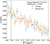 |
Fig. 1. θ2 plot on SGR 1935+2154 persistent emission. We used 25.5 h of high-quality data (see Sect. 3), which we show here in a single energy bin from 0.1 TeV to 10 TeV. We show the distribution of ON counts in blue and the background distribution in orange. The dashed line represents the θ2 cut used to evaluate the significance. No emission is detected. |
As we did not detect the source, we performed a 1D spectral analysis with the reflected-regions background method to estimate the 95% confidence level ULs, which we show in Fig. 2. We used ten logarithmically spaced bins between 0.1 TeV and 10 TeV and assumed a point-like source with a power law spectrum with photon index 2.5, an average value for tera-electronvolt sources that have not a known emission model in literature, already proposed by H.E.S.S. Collaboration (2021). The UL on the integrated flux in the 0.1 TeV to 10 TeV range is 5.6 ⋅ 10−12 s−1 cm−2, corresponding to 2.4 ⋅ 10−12 erg s−1 cm−2. The flux UL above 0.6 TeV, for direct comparison with H.E.S.S. Collaboration (2021), is 3.0 ⋅ 10−13 s−1 cm−2 (corresponding to 6.8 ⋅ 10−13 erg s−1 cm−2). We also searched for source variability by computing the nightly light curve of the emission and the nightly spectral energy distribution (SED, ≈2 h livetime per night), but we did not detect the source in any of the observation nights.
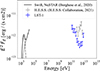 |
Fig. 2. Multi-band SED of the persistent emission of SGR 1935+2154. Black lines show the best fit emission model in the X-ray and soft gamma-ray bands (Borghese et al. 2022). In the VHE band, our 95% confidence level ULs confirm the non-detection obtained by H.E.S.S. Collaboration (2021). The tera-electronvolt ULs are about the same order of magnitude as the X-ray emission and confirm previous studies, which suggest that the power-law component observed above > 10 keV must have a break at MeV energies. |
For visualisation purposes we produced the excess and significance 2D maps centred on SGR 1935+2154, using the ring-background model in gammapy. Since the ring spans regions with offsets different from the ON region, the detector acceptance cannot be assumed to be constant, and its profile must therefore be computed explicitly (Berge et al. 2007). We evaluated the radial acceptance from the data on a run-by-run basis and stacked the results to estimate the background for the entire dataset (Abe et al. 2023a), using the BAccMod2 package. The position of SGR 1935+2154 was masked to prevent contamination. We defined the OFF region as a ring with internal radius of 0.5 deg and 0.3 deg width, around a 0.2 deg radius circular ON region. The maps, shown in Fig. 3, do not show any significant excess on the source.
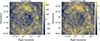 |
Fig. 3. Excess (left) and statistical significance (right) maps in a 3 deg × 3 deg region centred on SGR 1935+2154 in the 0.1 TeV to 10 TeV energy range. The ON region is shown as a white circle, while the background ring is delimited by the two dashed circles. The maps do not show any significant excess on the source. |
4. Bursting emission data analysis
To search for VHE bursting emission from SGR 1935+2154, we extracted a new dataset of photon lists and IRFs using a set of event selection cuts optimised to detect a gamma-ray signal on a 0.1 s timescale (typical duration of a short magnetar X-ray burst), in a low-photon-statistics regime and under the hypothesis of a Poisson background (Cowan 2007; Patrignani 2016; MAGIC Collaboration 2018). We used the following ‘burst cuts’: a cut in gammaness, gcut = 0.75, in intensity, icut = 50 p.e., and in θcut2 = 0.08 deg2.
The LST−1 observations included nine hard X-ray bursts from SGR 1935+2154 detected by various high-energy (HE) space telescopes (see Table 1). We searched for VHE counterpart emission simultaneous to these events, and also performed an unbiased search for short bursts in the whole dataset.
Upper limits in the [0.1−10] TeV range on known hard X-ray from SGR 1935+2154 observed by different satellites.
4.1. Search for tera-electronvolt emission simultaneous to X-ray bursts
We selected the nine LST−1 runs comprising the time of arrival (ToA) listed in Table 1, and the point-like IRFs for the closest simulation node to every run. We used the IRFs to obtain the exposure, assuming a power-law spectrum with index 2.
For each of the nine bursts listed in Table 1, we selected the number of photons, NON, in the ON region centred on SGR 1935+2154 (with size given by θcut), in a δt = 0.1 s time window centred around the ToA of each of the nine bursts, and in the 0.1 TeV to 10 TeV energy range. No timing correction was applied to the ToAs, which represent the detection times of the X-ray bursts. This choice is justified because all instruments in Table 1 are in low Earth orbit at altitudes of ≲600 km. The resulting time delay of the signal with respect to the LST−1 site is ≲2 ms, which is negligible compared to the 0.1 s analysis window.
None of the nine bursts is detected by LST−1, as NON is always lower than the N5σ threshold needed to claim a detection. The threshold depends on the measured background rate, Rbkg. The background rates of the nine selected observation runs are reported in Table 1, with the associated Poisson error.
The Bayesian treatment of the ON/OFF problem has been extensively discussed in the literature (e.g. Knoetig 2014; Casadei 2015). The number of counts in the ON region can be modelled with a Poisson likelihood, parametrised by the expected signal, s, and background, b, counts:
 (1)
(1)
where Poi denotes the Poisson distribution, and n is the statistical variable describing the ON counts (while we used NON for the actually measured values). Assuming statistical independence between s and b, the joint prior factorises as the product of the signal prior, πsig(s), and the background prior, πbkg(b). Once the priors have been derived, the UL to the signal parameter, sUL, can then be derived in three steps. First, the likelihood is marginalised over the background parameter:
 (2)
(2)
Then, the marginalised posterior distribution is obtained:
 (3)
(3)
Finally, the UL sUL at confidence level αCL is defined as the solution of
 (4)
(4)
The choice of priors for s and b is crucial in this approach and will now be examined. A common, though not always well-justified, approach is to assume a Dirac delta function for the background prior:
 (5)
(5)
where b0 is the expected background counts, usually estimated from the OFF region as b0 = α ⋅ NOFF, with α being the exposure ratio and NOFF the observed counts in the OFF region. A more general and statistically consistent approach, proposed by Casadei (2015), derives the background prior directly from the posterior distribution of the OFF region. The OFF region is described by a single Poisson likelihood, ℒOFF(k|B) = Poi(k; B), where k is the statistical variable and B the Poisson parameter. The prior for the OFF region can be naturally modelled as a Gamma distribution:
 (6)
(6)
where ν is the shape parameter, ρ the rate, and Γ the complete Gamma function. Since the Gamma distribution is conjugate to the Poisson model, the posterior for the OFF region is also Gamma-distributed, reading as
 (7)
(7)
By rescaling from the OFF to the ON region via the exposure ratio (b = α ⋅ B), the prior for the ON-region background becomes
 (8)
(8)
A well-known property of the Gamma distribution is that when both the shape and rate parameters tend to infinity, while their ratio b0 remains constant, the distribution converges to a Dirac delta function centred at b0. In Eq. (8), this ratio is given by
 (9)
(9)
In general, the choice of the shape and rate parameters define how the background is characterised. For example, adopting Jeffreys’ prior for πOFF(B) corresponds to setting ν = 1/2 and ρ = 0 (Casadei 2015). Since the best estimator for the expected value of k is the observed number of counts in the OFF region, NOFF, the shape-to-rate ratio can be estimated as b0 = α ⋅ (NOFF + 1/2).
If the selected OFF region satisfies α ≪ 1 and NOFF ≫ 1, the background prior, πbkg, in Eq. (8) tends to a Dirac delta with b0 ≈ α ⋅ NOFF (neglecting the 1/2 term), as in Eq. (10). Within this framework, and under these specific conditions, the use of a Dirac delta as background prior is not merely an ad hoc assumption, but can be justified as the approximation of a ‘well-characterised background’.
For our analysis, we selected a single OFF region, symmetrical to the ON region with respect to the pointing direction and of equal size. The exposure ratio is therefore given by the ratio of the observing times,  , where TON = 0.1 s and TOFF corresponds to the full duration of the observation run (≈15 − 20 min). This yields α ∼ 10−4, with measured OFF counts in the range of NOFF ≈ 500 − 1000 across the selected runs.
Our observations satisfy the conditions for the well-characterised background approximation, provided that the event rate remains constant, ensuring that the background can be described by a single Poisson distribution. In practice, the event rate is not perfectly constant due to variations in atmospheric conditions and telescope pointing during a run. To account for this, we tested all selected observations to verify that the distribution of binned OFF counts is consistent with a single Poisson law using a χ2 test, and rate variations are negligible.
As an example, Fig. 4 shows the distribution of binned OFF counts for the observation run of burst #1 in Table 1. The observed counts are consistent with the Poisson prediction, yielding a χ2 statistic of 3.1 for 3 degrees of freedom, corresponding to a p value of 0.3. Similar results for the other observation runs support the validity of the well-characterised background approximation. Under these conditions, we consider adopting Eq. (5) as the background prior to be justified.
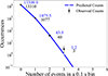 |
Fig. 4. Distribution of binned OFF counts (black points and labels) in the observation run of burst #1 of Table 1. The data are consistent with the expectation from a Poisson distribution (blue points, labels and line) with background rate RBKG = 0.81 s−1, using bins of width δt = 0.1 s. The total duration of the run was 1443 s. |
Once the background prior is fixed, the marginalised likelihood, ℒsig(n ∣ s), can be computed as in Eq. (2). Under the well-characterised background approximation, this reduces to the offset Poisson distribution Poi(n; s + b0), whereas in the general case it is proportional to an exponential times a polynomial (for a detailed discussion, see Casadei 2012, 2014).
Having established the treatment of the background prior and the resulting marginalised likelihood, we now turn to the choice of the signal prior, πsig(s). A common assumption is to adopt a uniform prior for s > 0, mainly for its mathematical simplicity (Cowan 2007; Patrignani 2016; MAGIC Collaboration 2018), and because it is often considered as a ‘non-informative’ prior. In reality, it does not result from a formal procedure for constructing an objective prior. Moreover, it disproportionately favours large values of the signal, even nonphysical large ones, which leads to an overestimation of both the posterior mean and the corresponding ULs (Casadei 2014).
By contrast, Jeffreys’ prior is derived solely from the Fisher information of the likelihood and can therefore be regarded as an objective prior. For an offset Poisson distribution, such as the marginalised likelihood ℒsig(n|s) = Poi(n; s + b0), it is
 (10)
(10)
which we adopted as our signal prior. It is important to note that Jeffreys’ prior depends on the marginalised likelihood, and therefore implicitly carries information from the background prior. If πbkg(b) is not a Dirac delta, the signal prior cannot be computed analytically. Eq. (10) should thus be regarded as the approximation of the general prior under the well-characterised background assumption (for a comparison of numerical and approximate priors, see Casadei 2014).
Once the signal prior and the marginalised likelihood are specified, the posterior distribution can be obtained by multiplication and normalisation, as in Eq. (3). The calculations are presented in Appendix A for completeness. Its explicit form is
![Mathematical equation: $$ \begin{aligned} {\mathcal{P} }_{\rm sig}(s|n) = \frac{(s+b_0)^{n-\frac{1}{2}} \, e^{-(s+b_0)}}{\Gamma \left(n+\frac{1}{2}\right) \cdot \left[1 - F_{\chi ^2} \left(2b_0; 2 n+1\right)\right]}, \end{aligned} $$](/articles/aa/full_html/2026/02/aa55431-25/aa55431-25-eq13.gif) (11)
(11)
where Fχ2 is the cumulative distribution function of the χ2 distribution with 2n + 1 degrees of freedom, and b0 the expected background counts. The UL on the expected signal counts, sUL, follows from Eq. (4):
 (12)
(12)
where Fχ2−1 is the inverse cumulative distribution (percent-point) function of the χ2 distribution with 2n + 1 degrees of freedom, b0 the expected background counts, and 1 − αCL is the confidence level. The calculations are presented in Appendix A for completeness. The choice of prior directly affects the degrees of freedom of the χ2 distribution: for Jeffreys’ prior the term is 2n + 1, whereas for a uniform prior it would be 2(n + 1). Consequently, ULs computed with the uniform prior are systematically larger than those obtained with Jeffreys’ prior, reflecting the fact that Jeffreys’ prior assigns monotonically decreasing weight to higher signal intensities.
We report the 95% confidence level ULs sUL for every burst in Table 1. The estimation of the UL in practice was performed through Eq. (12), using the measured counts in the ON region, NON, as an estimator for n, and b0 as the background rate, Rbkg, times 0.1 s. We computed the corresponding ULs on the integral flux by dividing sUL over the exposure of the time window. The average photon flux UL for a 0.1 s burst is (1.6 ± 0.5)⋅10−8 cm−2 s−1 and the average energy fluence UL is (1.2 ± 0.4)⋅10−9 erg cm−2.
We stacked the counts and the exposure of every burst window to compute the ULs on the total VHE burst activity of SGR 1935+2154, reported in Table 1 under the assumption of average background and effective area. The stacked photon flux UL on the bursting emission is then 2.7 ⋅ 10−9 cm−2 s−1.
4.2. Non-simultaneous burst search
We searched for possible SGR 1935+2154 short bursts in our dataset. We binned the ON-source events in 0.1 s bins starting at the beginning of each observation run. We evaluated if any of the bins showed a post-trial significance of five standard deviations (Li & Ma 1983; Bulgarelli et al. 2012; Brun et al. 2020), and we did not find any detection.
The mean and standard deviation of the background rates across the runs of our dataset are Rbkg = 0.9 ± 0.3 s−1, which provide pre-trial N5σ from 3 to 5. Differences in the runs can be attributed to different zenith angle, atmospheric conditions, and NSB levels. We performed the burst search across all our dataset, considering each 0.1 s time bin as a trial, with the total number of trials Ntrials = 1 355 170. The corrected post-trial  range from 5 to 8. The flux sensitivity for our non-simultaneous burst search can be evaluated by dividing the highest
  over the lowest 0.1 s exposure of our dataset, which is 1.296 ⋅ 108 cm2 s, providing a minimum detectable photon flux of 6.2 ⋅ 10−8 cm−2 s−1 in the 0.1 TeV to 10 TeV. Its value is higher than that of the analysis described in Sect. 4.1 due to the large number of trials.
5. Discussion
We analysed over 25 h of VHE gamma-ray observations of SGR 1935+2154 with the LST−1 during periods of known magnetar activity. We did not detect persistent or bursting emission from the source but we provide ULs that constrain its emission in the 0.1 TeV to 10 TeV energy range. We discuss below our constrains in the context of multi-wavelength observations of SGR 1935+2154 and its possible emission mechanisms.
5.1. Persistent emission
As is seen in Sect. 3, no persistent VHE signal is detected from SGR 1935+2154. In Fig. 2, we present the multi-band SED of SGR 1935+2154. Black lines show the best fit emission model in the X-ray and soft gamma-ray bands extracted from June 2020 observations of the source with Swift and NuSTAR. The model is composed of a black-body spectrum plus a power-law component (Borghese et al. 2022). In the VHE band, our ULs improve those by H.E.S.S. Collaboration (2021), extending the covered energy range down to 0.1 TeV and lowering them by factors of 2 to 5. The tera-electronvolt ULs are about the same order of magnitude of the X-ray emission of SGR 1935+2154, and are consistent with previous studies on the source, which suggest that the power-law component observed in the SED above > 10 keV must have a break at ∼MeV energies.
Most models explain the persistent emission of magnetars in the X-ray band using two components. The first one is the thermal emission arising from the NS surface and its thin atmosphere (Turolla et al. 2015). The second one is due to the presence of accelerated particles in a magnetosphere with a complex geometry, which can modify the emitted spectrum producing hard tails by resonant cyclotron scattering of the thermal photons (Thompson et al. 2002). More complex models include MC simulations to study the motions of charged particles flowing in twisted magnetic loops (e.g. Fernández & Thompson 2007; Beloborodov 2013). Current models can produce power-law emission spectra with a suppression above the MeV range, but the underlying mechanisms are not fully understood yet, mainly due to the lack of data in this energy range. The cut-off has not been observed yet, and ULs are of the order of ∼10−10 erg s−1 cm−2 in the MeV range (e.g. den Hartog et al. 2006) and ∼10−12 erg s−1 cm−2 in the GeV range (Li et al. 2017). Future facilities capable of observing at ∼1 MeV, such as the upcoming COSI satellite mission (Tomsick et al. 2024), may detect the power law cut-off and validate these models.
Magnetars might also be a possible component of the progenitors of FRBs (Cordes & Chatterjee 2019; Zhang 2023). For instance, FRB 121102 (Spitler et al. 2014) is associated with a persistent radio source (PRS, Chatterjee et al. 2017) and an optical counterpart classified as a low-metallicity star-forming dwarf galaxy (Tendulkar et al. 2017; Bassa et al. 2017). The PRS emission is not identified, but is likely due to synchrotron emission of relativistic electrons from a surrounding nebula (e.g. Murase et al. 2016; Marcote et al. 2017; Metzger et al. 2017; Bhattacharya et al. 2025), possibly a SNR, a pulsar wind nebula (PWN), or a hyper-accreting X-ray binary (Sridhar & Metzger 2022). The recent detection of a PRS for FRB 20190520B (Niu et al. 2022), FRB 20201124A (Bruni et al. 2024a), and FRB 20240114A (Bruni et al. 2024b) supports nebular models powered by a NS as being the origin of FRBs. Even though no HE counterparts of FRBs or their associated PRS have been detected (Scholz et al. 2017; Zhang 2024), the progenitors proposed may emit HE and VHE gamma-rays with mechanisms similar to known PWNe or SNRs. These models suggest that magnetars can be interesting targets for IACTs such as LST−1 and the upcoming arrays of the CTAO (Abe et al. 2025).
5.2. Bursting emission
In Sect. 4.1 and Table 1 we obtained the VHE ULs to the bursting emission of SGR 1935+2154 on a 0.1 s timescale, centred on the ToAs of simultaneous bursts. Burst fluences and spectral analyses are available in the literature only for the four bursts detected by Fermi-GBM and NICER, and we can compare their X-ray flux with the simultaneous VHE UL.
The brightest of these bursts is #1, detected by Fermi-GBM with T0 = 2021-07-07 00:33:31.67 (Hamburg et al. 2021a,b). It has a single peak with T90 ≈ 0.1 s and is best fit by a power-law function with index 0.54 ± 0.07 and an exponential HE cut-off at Epeak = 36.1 ± 0.3 keV, with an average photon flux of 289 ± 3 s−1 cm−2, average energy flux of 1.3 ± 0.2 ⋅ 10−5 erg s−1 cm−2, and fluence of 2.52 ± 0.03 ⋅ 10−6 erg cm−2 (10 keV to 1000 keV, T0 − 0.064 s to T0 + 0.128 s). The 0.1−10 TeV flux UL over 0.1 s is 1.1 ⋅ 10−8 erg s−1 cm−2 (see Table 1). We show in Fig. 5 the SED of burst #1 using the Fermi-GBM flux point and the VHE UL. It is the most robust SED of a magnetar burst with a sub-second timescale and simultaneous X-ray and VHE data, and it constrains the ratio between the VHE and X-ray flux to a factor of ≲10−3.
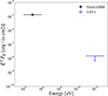 |
Fig. 5. Soft and VHE gamma-ray SED of the bursting emission of SGR 1935+2154 during the burst on July 7, 2021 00:33:31.670, measured on a ∼0.1 s timescale. |
Most magnetar models predict bursting emission in the X-ray and soft gamma-ray bands, either when magnetic stresses build up sufficiently to crack a patch of the NS crust, ejecting hot plasma into the magnetosphere (e.g. Thompson & Duncan 1995), or after magnetic reconnection events in the magnetosphere (Lyutikov 2002). Such models do not predict gamma-ray emission in the GeV–TeV energy ranges, but more complex magnetar models predict mechanism to emit FRBs accompanied by HE GeV–TeV bursts. For instance, Lyubarsky (2014) predicts that FRBs and strong millisecond bursts in the tera-electronvolt range can originate from the synchrotron maser emission caused by magnetised shocks that occur when highly magnetised plasma bursting from a magnetar reaches the medium surrounding the nebula.
Murase et al. (2016, 2017) suggested a scenario for the production of FRBs in which the spin-down power of a magnetar creates a relativistic wind bubble embedded in baryonic ejecta surrounding the NS, a scenario similar to PWNe. An impulsive energy injection of relativistic flow, which may originate from magnetic dissipation in the magnetosphere, may shock the nebula, causing the emission of a broadband flare observable from the radio band to the HE gamma-ray band. The fluence, φ, predicted for a HE gamma-ray flash (HEGF) in the fast cooling scenario (electrons and positrons cool within the dynamical time) at tera-electronvolt energies is
 (13)
(13)
where Eoutflow is the total energy of the burst outflow and d is the distance of the magnetar nebula. A TeV fluence UL of 1.1 ⋅ 10−9 erg cm−2 such as the one we obtained for the SGR 1935+2154 burst #1 would constrain the total energy of the burst outflow to Eoutflow ≲ 2.7 ⋅ 1037 erg assuming distance d = 4.4 kpc (Mereghetti et al. 2020). We stress that the model cannot be directly applied to burst #1 as it is a typical magnetar burst with no radio counterpart, and a softer index and peak energy with respect to the burst on April 2020 associated with radio bursts (Mereghetti et al. 2020). Furthermore, SGR 1935+2154 lacks the nebular structure that is required for a FRB-HEGF event (Murase et al. 2016). Nevertheless, other sources of FRBs may possess the structures required for HEGFs, and these theoretical models motivate the search for counterparts of FRBs and magnetar bursts and flares at VHE with IACTs (Carosi & López-Oramas 2024).
The detection of a candidate MGF in the nearby (3.5 Mpc) Sculptor galaxy at GeV energies (Fermi-LAT Collaboration 2021) also motivates the search for magnetar flares at HE and VHE. It was described by a power-law spectrum with index −1.7 ± 0.3 and integral flux above 0.1 GeV Φ(> 0.1 GeV) = (4.1 ± 2.2)×10−6 s−1 cm−2 (Fermi-LAT Collaboration 2021). Assuming that this power-law spectrum extends to tera-electronvolt energies, the estimated average flux above 0.1 TeV at the distance of SGR 1935+2154 would be approximately Φ(> 0.1 TeV)≃2.0 ⋅ 10−3 s−1 cm−2. The LST−1 sensitivity for a 0.1 s burst is ≃3 ⋅ 10−8 s−1 cm−2, suggesting that a short flare with the average flux of the MGF could be detected up to a distance of a few Mpc. However, the sensitivity can vary significantly depending on the source position (e.g. within or outside the Galactic plane), observing conditions, and flare duration. Furthermore, this estimate assumes that the spectrum measured by Fermi-LAT Collaboration (2021) extends to tera-electronvolt energies, which remains to be confirmed.
6. Conclusions
We analysed over 25 h of high-quality observations of magnetar SGR 1935+2154 with LST−1 in order to search for a VHE counterpart to its persistent or bursting emission. We did not detect the persistent emission of the source in the 0.1 TeV to 10 TeV energy range, in agreement with previous observations (H.E.S.S. Collaboration 2021), and as is implied by the MeV ULs, if there is only a single spectral component extending from X-rays to VHE. Our tera-electronvolt ULs are about the same order of magnitude as the X-ray emission of SGR 1935+2154.
We conducted our observations during periods of known bursting activity of the source, and simultaneously to nine short magnetar bursts detected by instruments sensitive to X-rays on board several space satellites. We searched for a transient VHE emission of SGR 1935+2154 that coincided with the HE bursts on a timescale of 0.1 s, in a low-photon-statistics regime and under the hypothesis of a Poisson background, optimising the event selection cuts for the analysis. For the first time, we provided the VHE flux ULs to the emission of a short magnetar burst (∼1.2 ⋅ 10−8 erg s−1 cm−2) simultaneous to its soft gamma-ray flux. For the brightest burst in our sample, the ratio between the VHE and X-ray flux is ≲10−3. We also searched for possible 0.1 s bursts in our dataset and we did not observe any significant signal.
Although no persistent or bursting emission has yet been detected at tera-electronvolt energies from SGR 1935+2154 and other magnetars, the detection of MeV–GeV emission and theoretical predictions of a VHE component in flares make magnetars and FRBs interesting candidate sources for IACTs and CTAO in particular. A flare with the same power-law spectrum as the candidate MGF detected in the Sculptor galaxy (Fermi-LAT Collaboration 2021) could have been within the detection capabilities of LST−1, assuming that the power law extends up to tera-electronvolt energies. A next-generation facility such as the CTAO will be particularly suited for fast transient astronomy thanks to its improved VHE sensitivity3 (approximately an order of magnitude greater than that of LST−1). This enhanced sensitivity, primarily attributed to the Large-Sized Telescopes (LSTs) in the low-energy range, will not only improve detection capabilities but also lower the energy threshold, enabling the CTAO to observe gamma-ray fluxes comparable to those expected from magnetar bursts and flares (Abe et al. 2025). The burst analysis method described in Sect. 4 is an alternative to the standard methods of Sect. 3 and is particularly useful for the analysis of fast transients such as FRBs, magnetar bursts and flares, and short gamma-ray bursts that may belong to a small-photon-statistics regime. Another key feature of CTAO in the context of transient astronomy will be its capability to swiftly react to external alerts from complementary astrophysical facilities by triggering target-of-opportunity observations. The CTAO will be able to swiftly re-point its telescopes and perform real-time analyses using its Science Alert Generation system (Di Piano et al. 2022; Bulgarelli et al. 2024), which is part of the Array Control and Data Acquisition of CTAO (Oya et al. 2024). A real-time analysis system has already been deployed for LST−1 to monitor nightly observations (Caroff et al. 2023).
References
- Abe, S., Aguasca-Cabot, A., Agudo, I., et al. 2023a, A&A, 673, A75 [NASA ADS] [CrossRef] [EDP Sciences] [Google Scholar]
- Abe, H., Abe, K., Abe, S., et al. 2023b, ApJ, 956, 80 [CrossRef] [Google Scholar]
- Abe, K., Abe, S., Abhir, J., et al. 2025, MNRAS, 540, 205 [Google Scholar]
- Acero, F., Aguasca-Cabot, A., Bernete, J., et al. 2025, https://doi.org/10.5281/zenodo.14760974 [Google Scholar]
- Aleksić, J., Antonelli, L. A., Antoranz, P., et al. 2013, A&A, 549, A23 [NASA ADS] [CrossRef] [EDP Sciences] [Google Scholar]
- Bailes, M., Bassa, C. G., Bernardi, G., et al. 2021, MNRAS, 503, 5367 [Google Scholar]
- Baring, M. G., & Harding, A. K. 2007, Ap&SS, 308, 109 [Google Scholar]
- Bassa, C. G., Tendulkar, S. P., Adams, E. A. K., et al. 2017, ApJ, 843, L8 [NASA ADS] [CrossRef] [Google Scholar]
- Beloborodov, A. M. 2013, ApJ, 762, 13 [NASA ADS] [CrossRef] [Google Scholar]
- Beloborodov, A. M., & Thompson, C. 2007, ApJ, 657, 967 [Google Scholar]
- Berge, D., Funk, S., & Hinton, J. 2007, A&A, 466, 1219 [CrossRef] [EDP Sciences] [Google Scholar]
- Bhattacharya, M., Murase, K., & Kashiyama, K. 2025, MNRAS, in press, https://doi.org/10.1093/mnras/staf2175 [Google Scholar]
- Bochenek, C. D., Ravi, V., Belov, K. V., et al. 2020, Nature, 587, 59 [NASA ADS] [CrossRef] [Google Scholar]
- Borghese, A., Coti Zelati, F., Israel, G. L., et al. 2022, MNRAS, 516, 602 [Google Scholar]
- Breiman, L. 2001, Mach. Learn., 45, 5 [Google Scholar]
- Brun, F., Piel, Q., de Naurois, M., & Bernhard, S. 2020, Astropart. Phys., 118, 102429 [NASA ADS] [CrossRef] [Google Scholar]
- Bruni, G., Piro, L., Yang, Y.-P., et al. 2024a, Nature, 632, 1014 [CrossRef] [Google Scholar]
- Bruni, G., Piro, L., Nicastro, L., et al. 2024b, ATel, 16885 [Google Scholar]
- Bulgarelli, A., Chen, A. W., Tavani, M., et al. 2012, A&A, 540, A79 [NASA ADS] [CrossRef] [EDP Sciences] [Google Scholar]
- Bulgarelli, A., Caroff, S., Castaldini, L., et al. 2024, SPIE Conf. Ser., 13101, 1310129 [Google Scholar]
- Cai, C., Xiong, S. L., Huang, Y., et al. 2021, GRB Coordinates Network, 30836 [Google Scholar]
- Caroff, S., Aubert, P., Garcia, E., et al. 2023, ArXiv e-prints [arXiv:2309.11679] [Google Scholar]
- Carosi, A., & López-Oramas, A. 2024, Universe, 10, 163 [Google Scholar]
- Casadei, D. 2012, J. Instrum., 7, 1012 [Google Scholar]
- Casadei, D. 2014, J. Instrum., 9, T10006 [Google Scholar]
- Casadei, D. 2015, ApJ, 798, 5 [Google Scholar]
- Chatterjee, S., Law, C. J., Wharton, R. S., et al. 2017, Nature, 541, 58 [NASA ADS] [CrossRef] [Google Scholar]
- CHIME/FRB Collaboration (Andersen, B. C., et al.) 2020, Nature, 587, 54 [Google Scholar]
- Cordes, J. M., & Chatterjee, S. 2019, ARA&A, 57, 417 [NASA ADS] [CrossRef] [Google Scholar]
- Coti Zelati, F., Rea, N., Pons, J. A., Campana, S., & Esposito, P. 2018, MNRAS, 474, 961 [NASA ADS] [CrossRef] [Google Scholar]
- Cowan, G. 2007, ASP Conf. Ser., 371, 75 [Google Scholar]
- CTA (Abe, K., et al.) 2024, 38th International Cosmic Ray Conference, 703 [Google Scholar]
- den Hartog, P. R., Hermsen, W., Kuiper, L., et al. 2006, A&A, 451, 587 [NASA ADS] [CrossRef] [EDP Sciences] [Google Scholar]
- Denissenya, M., Grossan, B., & Linder, E. V. 2021, Phys. Rev. D, 104, 023007 [NASA ADS] [CrossRef] [Google Scholar]
- Di Piano, A., Bulgarelli, A., Fioretti, V., et al. 2022, 37th International Cosmic Ray Conference, 694 [Google Scholar]
- Donath, A., Terrier, R., Remy, Q., et al. 2023, A&A, 678, A157 [NASA ADS] [CrossRef] [EDP Sciences] [Google Scholar]
- Feigelson, E. D., & Babu, G. J. 2012, Modern Statistical Methods for Astronomy: With R Applications (Cambridge: Cambridge University Press) [Google Scholar]
- Fermi-LAT Collaboration (Ajello, M., et al.) 2021, Nat. Astron., 5, 385 [CrossRef] [Google Scholar]
- Fernández, R., & Thompson, C. 2007, ApJ, 660, 615 [CrossRef] [Google Scholar]
- Fomin, V., Stepanian, A., Lamb, R., et al. 1994, Astropart. Phys., 2, 137 [NASA ADS] [CrossRef] [Google Scholar]
- Garcia, E., Vuillaume, T., & Nickel, L. 2022, ArXiv e-prints [arXiv:2212.00120] [Google Scholar]
- Ge, M. Y., Liu, C. Z., Zhang, S. N., et al. 2023, ApJ, 953, 67 [Google Scholar]
- Guver, T., Hu, C.-P., Younes, G., et al. 2021, ATel, 14916 [Google Scholar]
- H.E.S.S. Collaboration (Abdalla, H., et al.) 2021, ApJ, 919, 106 [NASA ADS] [CrossRef] [Google Scholar]
- Hamburg, R., Malacaria, C., & Fletcher, C. 2021a, ATel, 14764 [Google Scholar]
- Hamburg, R., Malacaria, C., Fletcher, C., & Fermi GBM Team 2021b, GRB Coordinates Network, 30407 [Google Scholar]
- Hillas, A. M. 1985, 19th International Cosmic Ray Conference (ICRC19), 3, 445 [NASA ADS] [Google Scholar]
- Hurley, K., Cline, T., Mazets, E., et al. 1999, Nature, 397, 41 [NASA ADS] [CrossRef] [Google Scholar]
- Israel, G., & Dall’Osso, S. 2011, High-Energy Emission from Pulsars and their Systems (Berlin, Heidelberg: Springer), 279 [Google Scholar]
- Israel, G. L., Esposito, P., Rea, N., et al. 2016, MNRAS, 457, 3448 [NASA ADS] [CrossRef] [Google Scholar]
- Kaspi, V. M., & Beloborodov, A. M. 2017, ARA&A, 55, 261 [Google Scholar]
- Knoetig, M. L. 2014, ApJ, 790, 106 [NASA ADS] [CrossRef] [Google Scholar]
- Kothes, R., Sun, X., Gaensler, B., & Reich, W. 2018, ApJ, 852, 54 [NASA ADS] [CrossRef] [Google Scholar]
- Kozlova, A. V., Israel, G. L., Svinkin, D. S., et al. 2016, MNRAS, 460, 2008 [NASA ADS] [CrossRef] [Google Scholar]
- Li, T. P., & Ma, Y. Q. 1983, ApJ, 272, 317 [CrossRef] [Google Scholar]
- Li, J., Rea, N., Torres, D. F., & de Oña-Wilhelmi, E. 2017, ApJ, 835, 30 [Google Scholar]
- Li, C. K., Lin, L., Xiong, S. L., et al. 2021, Nat. Astron., 5, 378 [NASA ADS] [CrossRef] [Google Scholar]
- Lin, L., Göğüş, E., Roberts, O. J., et al. 2020a, ApJ, 893, 156 [CrossRef] [Google Scholar]
- Lin, L., Göğüş, E., Roberts, O. J., et al. 2020b, ApJ, 898, 176 [Google Scholar]
- Lin, L., Göğüş, E., Roberts, O. J., et al. 2020c, ApJ, 902, L43 [NASA ADS] [CrossRef] [Google Scholar]
- López-Coto, R., Moralejo, A., Artero, M., et al. 2021, Proceedings, 37th International Cosmic Ray Conference, 395, 806 [Google Scholar]
- Lopez-Coto, R., Vuillaume, T., Moralejo, A., et al. 2023, https://doi.org/10.5281/zenodo.7565826 [Google Scholar]
- López-Oramas, A., Jiménez Martínez, I., Hassan, T., et al. 2022, 37th International Cosmic Ray Conference, 783 [Google Scholar]
- Lyubarsky, Y. 2014, MNRAS, 442, L9 [Google Scholar]
- Lyutikov, M. 2002, ApJ, 580, L65 [NASA ADS] [CrossRef] [Google Scholar]
- MAGIC Collaboration (Acciari, V. A., et al.) 2018, MNRAS, 481, 2479 [Google Scholar]
- Marcote, B., Paragi, Z., Hessels, J. W. T., et al. 2017, ApJ, 834, L8 [CrossRef] [Google Scholar]
- Mazets, E. P., Golentskii, S. V., Ilinskii, V. N., Aptekar, R. L., & Guryan, I. A. 1979, Nature, 282, 587 [NASA ADS] [CrossRef] [Google Scholar]
- Mereghetti, S., Pons, J. A., & Melatos, A. 2015, Space Sci. Rev., 191, 315 [NASA ADS] [CrossRef] [Google Scholar]
- Mereghetti, S., Savchenko, V., Ferrigno, C., et al. 2020, ApJ, 898, L29 [Google Scholar]
- Mereghetti, S., Rigoselli, M., Salvaterra, R., et al. 2024, Nature, 629, 58 [NASA ADS] [CrossRef] [Google Scholar]
- Metzger, B. D., Berger, E., & Margalit, B. 2017, ApJ, 841, 14 [NASA ADS] [CrossRef] [Google Scholar]
- Morcuende, D., Ruiz, J. E., Saha, L., et al. 2022, https://doi.org/10.5281/zenodo.7263048 [Google Scholar]
- Murase, K., Kashiyama, K., & Mészáros, P. 2016, MNRAS, 461, 1498 [NASA ADS] [CrossRef] [Google Scholar]
- Murase, K., Kashiyama, K., & Mészáros, P. 2017, MNRAS, 467, 3542 [Google Scholar]
- Nakahira, S., Yoshida, A., Sakamoto, T., et al. 2021, GRB Coordinates Network, 30458 [Google Scholar]
- Nigro, C., Hassan, T., & Olivera-Nieto, L. 2021, Universe, 7, 374 [NASA ADS] [CrossRef] [Google Scholar]
- Niu, C. H., Aggarwal, K., Li, D., et al. 2022, Nature, 606, 873 [NASA ADS] [CrossRef] [Google Scholar]
- Olausen, S. A., & Kaspi, V. M. 2014, ApJS, 212, 6 [Google Scholar]
- Olive, J.-F., Hurley, K., Sakamoto, T., et al. 2004, ApJ, 616, 1148 [Google Scholar]
- Oya, I., Aubert, P., Baroncelli, L., et al. 2024, SPIE Conf. Ser., 13101, 131011D [Google Scholar]
- Palmer, D. M., Barthelmy, S., Gehrels, N., et al. 2005, Nature, 434, 1107 [NASA ADS] [CrossRef] [Google Scholar]
- Patrignani, C. 2016, Chin. Phys. C, 40, 100001 [Google Scholar]
- Petroff, E., Hessels, J. W. T., & Lorimer, D. R. 2019, A&ARv, 27, 4 [NASA ADS] [CrossRef] [Google Scholar]
- Rehan, N. U. S., & Ibrahim, A. I. 2023, ApJ, 950, 121 [Google Scholar]
- Ridnaia, A., Svinkin, D., Frederiks, D., et al. 2021a, Nat. Astron., 5, 372 [NASA ADS] [CrossRef] [Google Scholar]
- Ridnaia, A., Frederiks, D., Golenetskii, S., et al. 2021b, GRB Coordinates Network, 30418 [Google Scholar]
- Roberts, O. J., & Fermi GBM Team 2021, GRB Coordinates Network, 30831 [Google Scholar]
- Roberts, O. J., & Wood, J. 2021, ATel, 14907 [Google Scholar]
- Roberts, O. J., Wood, J., & Fermi GBM Team 2021, GRB Coordinates Network, 30806 [Google Scholar]
- Ruiz, J. E., Morcuende, D., Saha, L., et al. 2022, ASP Conf. Ser., 532, 369 [Google Scholar]
- Scholz, P., Bogdanov, S., Hessels, J. W. T., et al. 2017, ApJ, 846, 80 [NASA ADS] [CrossRef] [Google Scholar]
- Spitler, L. G., Cordes, J. M., Hessels, J. W. T., et al. 2014, ApJ, 790, 101 [NASA ADS] [CrossRef] [Google Scholar]
- Sridhar, N., & Metzger, B. D. 2022, ApJ, 937, 5 [NASA ADS] [CrossRef] [Google Scholar]
- Tavani, M., Casentini, C., Ursi, A., et al. 2021, Nat. Astron., 5, 401 [NASA ADS] [CrossRef] [Google Scholar]
- Tendulkar, S. P., Bassa, C. G., Cordes, J. M., et al. 2017, ApJ, 834, L7 [NASA ADS] [CrossRef] [Google Scholar]
- Thompson, C., & Beloborodov, A. M. 2005, ApJ, 634, 565 [Google Scholar]
- Thompson, C., & Duncan, R. C. 1995, MNRAS, 275, 255 [Google Scholar]
- Thompson, C., Lyutikov, M., & Kulkarni, S. R. 2002, ApJ, 574, 332 [NASA ADS] [CrossRef] [Google Scholar]
- Tomsick, J., Boggs, S., Zoglauer, A., et al. 2024, 38th International Cosmic Ray Conference, 745 [Google Scholar]
- Turolla, R., Zane, S., & Watts, A. L. 2015, Rep. Progr. Phys., 78, 116901 [Google Scholar]
- Vuillaume, T., Garcia, E., & Nickel, L. 2023, https://doi.org/10.5281/zenodo.7833122 [Google Scholar]
- Xiao, S., Huang, Y., Zhao, X. Y., et al. 2021, GRB Coordinates Network, 30400 [Google Scholar]
- Xue, W. C., Xiong, S. L., Cai, C., et al. 2021, GRB Coordinates Network, 30822 [Google Scholar]
- Zhang, B. 2023, Rev. Mod. Phys., 95, 035005 [NASA ADS] [CrossRef] [Google Scholar]
- Zhang, B. 2024, Annu. Rev. Nucl. Part. Sci., 74, 89 [Google Scholar]
- Zhou, P., Zhou, X., Chen, Y., et al. 2020, ApJ, 905, 99 [NASA ADS] [CrossRef] [Google Scholar]
Appendix A: Solution of the upper limit equation
For completeness, we provide the intermediate steps needed to obtain the explicit form of the posterior distribution 𝒫sig(s|n) in eq. (11), starting from its definition in eq. (3), and the UL equation eq. (12) in Sect. 4.1. The derivations rely on the definition of the complete Gamma function
 (A.1)
(A.1)
the lower incomplete Gamma function
 (A.2)
(A.2)
and their property
 (A.3)
(A.3)
where Fχ2 denotes the cumulative distribution function of a χ2 distribution with 2y degrees of freedom (see e.g. Feigelson & Babu 2012).
A.1. Posterior Distribution
The explicit form of the marginalised likelihood follows from eq. (2) when the background prior is taken to be a Dirac delta, eq. (5):
 (A.4)
(A.4)
We use eq. (A.4) and eq. (10) to evaluate the normalisation in the denominator of eq. (3):
![Mathematical equation: $$ \begin{aligned}&\int _{0}^{\infty } \, \pi _{\mathrm{sig} } (s)\, {\fancyscript {L}}_{\mathrm{sig} }(n|s) \, \mathrm{d}s = \int _{0}^{\infty } \, \sqrt{\frac{b_0}{s+b_0}} \frac{(s+b_0)^n}{n!} e^{-(s+b_0)} \, \mathrm{d}s = \frac{b_0^{\frac{1}{2}}}{n!} \int _0^\infty \, (s+b_0)^{n-\frac{1}{2}} e^{-(s+b_0)} \, \mathrm{d}s \underset{{t=s+b_0}}{=} \frac{b_{0}^{\frac{1}{2}}}{n!} \int _{b_{0}}^{\infty } \, t^{n-\frac{1}{2}} e^{-t} \, \mathrm{d}t =\nonumber \\&= \frac{b_{0}^{\frac{1}{2}}}{n!} \left(\int _{0}^{\infty } \, t^{n-\frac{1}{2}} e^{-t} \, \mathrm{d}t - \int _{0}^{b_{0}} \, t^{n-\frac{1}{2}} e^{-t} \, \mathrm{d}t\right) = \frac{b_{0}^{\frac{1}{2}}}{n!} \left[\Gamma \left(n+\frac{1}{2}\right) - \gamma \left(n+\frac{1}{2}, b_{0}\right) \right] \underset{{\mathrm{Eq.\ (A.3)} }}{=} \frac{b_{0}^{\frac{1}{2}}}{n!} \left[\Gamma \left(n+\frac{1}{2}\right) - \Gamma \left(n+\frac{1}{2}\right) \cdot F_{\chi ^{2}} \left(2b_{0}; 2n+1\right)\right]\nonumber \\&= \frac{b_0^{\frac{1}{2}}}{n!} \cdot \Gamma \left(n+\frac{1}{2}\right) \cdot \left[1 - F_{\chi ^2} \left(2b_0; 2n+1\right)\right]. \end{aligned} $$](/articles/aa/full_html/2026/02/aa55431-25/aa55431-25-eq22.gif) (A.5)
(A.5)
Substituting this result into eq. (3) and simplifying shows that the prefactor  cancels, leading directly to the posterior in eq. (11).
A.2. Upper limit
The derivation of the Bayesian UL in eq. (12) proceeds in a similar way. Starting from its definition, eq. (4), we have
![Mathematical equation: $$ \begin{aligned} 1-\alpha _{\mathrm{CL} }&= \int _{0}^{s_{\mathrm{UL} }} \, {\mathcal{P} }_{\mathrm{sig} }(s|n) \, \mathrm{d}s = \frac{ \int _{0}^{s_{\mathrm{UL} }} \, (s+b_0)^{n-\frac{1}{2}} \, e^{-(s+b_0)} \, \mathrm{d}s}{\Gamma \left(n+\frac{1}{2}\right) \cdot \left[1 - F_{\chi ^2} \left(2 b_0; 2n+1\right) \right]} = \frac{ \int _{b_{0}}^{s_{\mathrm{UL} }+b_0} \, t^{n-\frac{1}{2}} e^{-t} \, \mathrm{d}t}{\Gamma \left(n+\frac{1}{2}\right) \cdot \left[1 - F_{\chi ^2} \left(2 b_0; 2n+1\right)\right]}=\nonumber \\&= \frac{\int _{0}^{s_{\mathrm{UL} }+b_0} \, t^{n-\frac{1}{2}} e^{-t} \, \mathrm{d}t - \int _{0}^{b_0} \, t^{n-\frac{1}{2}} e^{-t} \, \mathrm{d}t}{\Gamma \left(n+\frac{1}{2}\right) \cdot \left[1 - F_{\chi ^2} \left(2 b_0; 2n+1\right)\right]} = \frac{\gamma \left(n+\frac{1}{2}, s_{\mathrm{UL} }+b_0\right) - \gamma \left(n+\frac{1}{2}, b_0\right)}{\Gamma \left(n+\frac{1}{2}\right) \cdot \left[ 1 - F_{\chi ^2} \left(2 b_0; 2n+1\right)\right]} =\frac{F_{\chi ^2} \left( 2 \left(s_{\mathrm{UL} }+b_0\right); 2n+1\right) - F_{\chi ^2} \left(2 b_0; 2n+1\right)}{1 - F_{\chi ^2} \left(2 b_0; 2n+1\right)}. \end{aligned} $$](/articles/aa/full_html/2026/02/aa55431-25/aa55431-25-eq24.gif) (A.6)
(A.6)
Rearranging, we obtain the equivalent condition:
![Mathematical equation: $$ \begin{aligned} F_{\chi ^2} \left(2\left(s_{\mathrm{UL} }+b_0\right); 2n+1\right)&= \left(1- \alpha _{\mathrm{CL} }\right) \cdot \left[1 - F_{\chi ^2} \left(2 b_0; 2n+1\right)\right] + F_{\chi ^2} \left(2 b_0; 2n+1\right), \end{aligned} $$](/articles/aa/full_html/2026/02/aa55431-25/aa55431-25-eq25.gif) (A.7)
(A.7)
![Mathematical equation: $$ \begin{aligned} F_{\chi ^2} \left(2\left(s_{\mathrm{UL} }+b_0\right); 2n+1\right)&= 1 -\alpha _{\mathrm{CL} } \cdot \left[1 - F_{\chi ^2} \left(2 b_0; 2n+1\right)\right],\end{aligned} $$](/articles/aa/full_html/2026/02/aa55431-25/aa55431-25-eq26.gif) (A.8)
(A.8)
![Mathematical equation: $$ \begin{aligned} 2\left(s_{\mathrm{UL} }+b_0\right)&= F_{\chi ^2}^{-1}\left(1 -\alpha _{\mathrm{CL} } \cdot \left[1 - F_{\chi ^2} \left(2 b_0; 2n+1\right)\right]; 2n+1\right). \end{aligned} $$](/articles/aa/full_html/2026/02/aa55431-25/aa55431-25-eq27.gif) (A.9)
(A.9)
From this result we can determine sUL directly, leading to eq. (12).
Appendix B: Acknowledgments
Acknowledgments. We gratefully acknowledge financial support from the following agencies and organisations: Conselho Nacional de Desenvolvimento Científico e Tecnológico (CNPq) Grant 309053/2022-6 and Fundação de Amparo à Pesquisa do Estado do Rio de Janeiro (FAPERJ) Grants E-26/200.532/2023 and E-26/211.342/2021, Fundação de Amparo à Pesquisa do Estado de São Paulo (FAPESP), Fundação de Apoio à Ciência, Tecnologia e Inovação do Paraná - Fundação Araucária, Ministry of Science, Technology, Innovations and Communications (MCTIC), Brasil; Ministry of Education and Science, National RI Roadmap Project DO1-153/28.08.2018, Bulgaria; Croatian Science Foundation (HrZZ) Project IP-2022-10-4595, Rudjer Boskovic Institute, University of Osijek, University of Rijeka, University of Split, Faculty of Electrical Engineering, Mechanical Engineering and Naval Architecture, University of Zagreb, Faculty of Electrical Engineering and Computing, Croatia; Ministry of Education, Youth and Sports, MEYS LM2023047, EU/MEYS CZ.02.1.01/0.0/0.0/16_013/0001403, CZ.02.1.01/0.0/0.0/18_046/0016007, CZ.02.1.01/0.0/0.0/16_019/0000754, CZ.02.01.01/00/22_008/0004632 and CZ.02.01.01/00/23_015/0008197 Czech Republic; CNRS-IN2P3, the French Programme d’investissements d’avenir and the Enigmass Labex, This work has been done thanks to the facilities offered by the Univ. Savoie Mont Blanc - CNRS/IN2P3 MUST computing center, France; Max Planck Society, German Bundesministerium für Forschung, Technologie und Raumfahrt (Verbundforschung / ErUM), the Deutsche Forschungsgemeinschaft (SFB 1491) and the Lamarr-Institute for Machine Learning and Artificial Intelligence, Germany; Istituto Nazionale di Astrofisica (INAF), Istituto Nazionale di Fisica Nucleare (INFN), Italian Ministry for University and Research (MUR), and the financial support from the European Union – Next Generation EU under the project IR0000012 - CTA+ (CUP C53C22000430006), announcement N.3264 on 28/12/2021: “Rafforzamento e creazione di IR nell’ambito del Piano Nazionale di Ripresa e Resilienza (PNRR)”; ICRR, University of Tokyo, JSPS, MEXT, Japan; JST SPRING - JPMJSP2108; Narodowe Centrum Nauki, grant number 2023/50/A/ST9/00254, Poland; The Spanish groups acknowledge the Spanish Ministry of Science and Innovation and the Spanish Research State Agency (AEI) through the government budget lines PGE2022/28.06.000X.711.04, 28.06.000X.411.01 and 28.06.000X.711.04 of PGE 2023, 2024 and 2025, and grants PID2019-104114RB-C31, PID2019-107847RB-C44, PID2019-105510GB-C31, PID2019-104114RB-C33, PID2019-107847RB-C43, PID2019-107847RB-C42, PID2019-107988GB-C22, PID2021-124581OB-I00, PID2021-125331NB-I00, PID2022-136828NB-C41, PID2022-137810NB-C22, PID2022-138172NB-C41, PID2022-138172NB-C42, PID2022-138172NB-C43, PID2022-139117NB-C41, PID2022-139117NB-C42, PID2022-139117NB-C43, PID2022-139117NB-C44, PID2022-136828NB-C42, PID2024-155316NB-I00, PDC2023-145839-I00 funded by the Spanish MCIN/AEI/10.13039/501100011033 and by ERDF/EU and NextGenerationEU PRTR; CSIC PIE 202350E189; the "Centro de Excelencia Severo Ochoa" program through grants no. CEX2020-001007-S, CEX2021-001131-S, CEX2024-001442-S; the "Unidad de Excelencia María de Maeztu" program through grants no. CEX2019-000918-M, CEX2020-001058-M; the "Ramón y Cajal" program through grants RYC2021-032991-I funded by MICIN/AEI/10.13039/501100011033 and the European Union “NextGenerationEU”/PRTR and RYC2020-028639-I; the "Juan de la Cierva-Incorporación" program through grant no. IJC2019-040315-I and "Juan de la Cierva-formación" through grant JDC2022-049705-I; the “Viera y Clavijo” postdoctoral program of Universidad de La Laguna, funded by the Agencia Canaria de Investigación, Innovación y Sociedad de la Información. They also acknowledge the "Atracción de Talento" program of Comunidad de Madrid through grant no. 2019-T2/TIC-12900; “MAD4SPACE: Desarrollo de tecnologías habilitadoras para estudios del espacio en la Comunidad de Madrid" (TEC-2024/TEC-182) project, Doctorado Industrial (IND2024/TIC34250) and Ayudas para la contratación de personal investigador predoctoral en formación (PIPF-2023/TEC-29694) funded by Comunidad de Madrid; the La Caixa Banking Foundation, grant no. LCF/BQ/PI21/11830030; Junta de Andalucía under Plan Complementario de I+D+I (Ref. AST22_0001) and Plan Andaluz de Investigación, Desarrollo e Innovación as research group FQM-322; Project ref. AST22_00001_9 with funding from NextGenerationEU funds; the “Ministerio de Ciencia, Innovación y Universidades” and its “Plan de Recuperación, Transformación y Resiliencia”; “Consejería de Universidad, Investigación e Innovación” of the regional government of Andalucía and “Consejo Superior de Investigaciones Científicas”, Grant CNS2023-144504 funded by MICIU/AEI/10.13039/501100011033 and by the European Union NextGenerationEU/PRTR, the European Union’s Recovery and Resilience Facility-Next Generation, in the framework of the General Invitation of the Spanish Government’s public business entity Red.es to participate in talent attraction and retention programmes within Investment 4 of Component 19 of the Recovery, Transformation and Resilience Plan; Junta de Andalucía under Plan Complementario de I+D+I (Ref. AST22_00001), Plan Andaluz de Investigación, Desarrollo e Innovación (Ref. FQM-322). “Programa Operativo de Crecimiento Inteligente" FEDER 2014-2020 (Ref. ESFRI-2017-IAC-12), Ministerio de Ciencia e Innovación, 15% co-financed by Consejería de Economía, Industria, Comercio y Conocimiento del Gobierno de Canarias; the "CERCA" program and the grants 2021SGR00426 and 2021SGR00679, all funded by the Generalitat de Catalunya; and the European Union’s NextGenerationEU (PRTR-C17.I1). This work is funded/Co-funded by the European Union (ERC, MicroStars, 101076533). This research used the computing and storage resources provided by the Port d’Informació Científica (PIC) data center. State Secretariat for Education, Research and Innovation (SERI) and Swiss National Science Foundation (SNSF), Switzerland; The research leading to these results has received funding from the European Union’s Seventh Framework Programme (FP7/2007-2013) under grant agreements No 262053 and No 317446; This project is receiving funding from the European Union’s Horizon 2020 research and innovation programs under agreement No 676134; ESCAPE - The European Science Cluster of Astronomy & Particle Physics ESFRI Research Infrastructures has received funding from the European Union’s Horizon 2020 research and innovation programme under Grant Agreement no. 824064.
Software used. lstchain v0.9.13 (López-Coto et al. 2021; Lopez-Coto et al. 2023), Gammapy v1.3 (Donath et al. 2023; Acero et al. 2025), lstMCpipe v0.10.0 (Garcia et al. 2022; Vuillaume et al. 2023), LSTOSA v0.9.2 (Ruiz et al. 2022; Morcuende et al. 2022).
Author Contributions. G. Panebianco: project coordination, LST–s data analysis, statistical methods, burst analysis pipeline development, results discussion and interpretation. A. López-Oramas: PI of the proposal, campaign and strategy coordinator. S. Mereghetti: results discussion and interpretation, paper drafting and editing. A. Simongini: LST–s data analysis. A. Bulgarelli: project supervision, paper drafting and editing. P. Bordas: project coordination. A. Carosi: LST–s data analysis supervision. A. Di Piano: statistical methods, paper drafting and editing. T. Hassan: burst analysis methods. I. Jiménez Martínez, paper drafting and editing. R. López-Coto: LST–s persistent emission data analysis. N. Parmiggiani: statistical methods, paper drafting and editing. C. Vignali: project supervision, paper drafting and editing. R. Zanin: project coordination. All authors above have participated in the paper discussion and edition. The rest of the authors have contributed in one or several of the following ways: design, construction, maintenance and operation of the instrument(s) used to acquire the data; preparation and/or evaluation of the observation proposals; data acquisition, processing, calibration and/or reduction; production of analysis tools and/or related MC simulations; discussion and approval of the contents of the draft. We kindly thank the anonymous referee and the CTAO internal reviewers for their careful reading and constructive comments, which helped improve the quality of this work.
All Tables
Upper limits in the [0.1−10] TeV range on known hard X-ray from SGR 1935+2154 observed by different satellites.
All Figures
|
Fig. 1. θ2 plot on SGR 1935+2154 persistent emission. We used 25.5 h of high-quality data (see Sect. 3), which we show here in a single energy bin from 0.1 TeV to 10 TeV. We show the distribution of ON counts in blue and the background distribution in orange. The dashed line represents the θ2 cut used to evaluate the significance. No emission is detected. |
| In the text | |
|
Fig. 2. Multi-band SED of the persistent emission of SGR 1935+2154. Black lines show the best fit emission model in the X-ray and soft gamma-ray bands (Borghese et al. 2022). In the VHE band, our 95% confidence level ULs confirm the non-detection obtained by H.E.S.S. Collaboration (2021). The tera-electronvolt ULs are about the same order of magnitude as the X-ray emission and confirm previous studies, which suggest that the power-law component observed above > 10 keV must have a break at MeV energies. |
| In the text | |
|
Fig. 3. Excess (left) and statistical significance (right) maps in a 3 deg × 3 deg region centred on SGR 1935+2154 in the 0.1 TeV to 10 TeV energy range. The ON region is shown as a white circle, while the background ring is delimited by the two dashed circles. The maps do not show any significant excess on the source. |
| In the text | |
|
Fig. 4. Distribution of binned OFF counts (black points and labels) in the observation run of burst #1 of Table 1. The data are consistent with the expectation from a Poisson distribution (blue points, labels and line) with background rate RBKG = 0.81 s−1, using bins of width δt = 0.1 s. The total duration of the run was 1443 s. |
| In the text | |
|
Fig. 5. Soft and VHE gamma-ray SED of the bursting emission of SGR 1935+2154 during the burst on July 7, 2021 00:33:31.670, measured on a ∼0.1 s timescale. |
| In the text | |
Current usage metrics show cumulative count of Article Views (full-text article views including HTML views, PDF and ePub downloads, according to the available data) and Abstracts Views on Vision4Press platform.
Data correspond to usage on the plateform after 2015. The current usage metrics is available 48-96 hours after online publication and is updated daily on week days.
Initial download of the metrics may take a while.