| Issue |
A&A
Volume 706, February 2026
|
|
|---|---|---|
| Article Number | A346 | |
| Number of page(s) | 11 | |
| Section | Numerical methods and codes | |
| DOI | https://doi.org/10.1051/0004-6361/202555462 | |
| Published online | 24 February 2026 | |
Multi-band neural network classification of ZTF light curves as LSST proxies
1
Konkoly Observatory, HUN-REN Research Centre for Astronomy and Earth Sciences,
Konkoly Thege Miklós út 15-17,
1121
Budapest,
Hungary
2
HUN-REN CSFK, MTA Centre of Excellence,
Konkoly Thege Miklós út 15–17,
1121
Budapest,
Hungary
3
Department of Astrophysical Sciences, Princeton University Peyton Hall,
4 Ivy Lane,
Princeton,
NJ
08544,
USA
4
ELTE Eötvös Loránd University, Institute of Physics and Astronomy,
Pázmány Péter sétány 1/a,
1117
Budapest,
Hungary
5
MTA–HUN-REN CSFK Lendület “Momentum” Stellar Pulsation Research Group,
Konkoly Thege Miklós út 15–17,
1121
Budapest,
Hungary
★ Corresponding author: This email address is being protected from spambots. You need JavaScript enabled to view it.
Received:
9
May
2025
Accepted:
11
December
2025
Abstract
Context. Current and near-future sky survey programmes, such as the Legacy Survey of Space and Time (LSST) of the Vera C. Rubin Observatory, will produce vast amounts of data that will need new techniques to process them on reasonable timescales. Machine-learning methods and properly trained neural networks proved to be efficient, fast, and reliable in performing a variety of tasks, such as the classification of variable star light curves. Since LSST survey full sky data are not yet available (only the data preview 1 from various sky segments), we tested our methods that are to be used on real LSST data on proxy datasets.
Aims. In this project, we used data obtained by the Zwicky Transient Facility to develop and test a neural-network-based multiband classification algorithm for classifying periodic variable stars (i.e. pulsating variable stars and eclipsing binaries). The aim is to use the algorithm on LSST data when they become available.
Methods. Phase-folded light-curve images and period information were used from five different variable star types: Classical and Type II Cepheids, δ Scuti stars, eclipsing binaries, and RR Lyrae stars. The data were taken from the 17th data release of ZTF, from which we used two passbands, g and r, in this project. The periods were calculated from the raw data, and this information was used as an additional numerical input in the neural network. For the training and testing process, a supervised machine-learning method was created. The neural network contained convolutional neural networks concatenated with fully connected layers.
Results. During the training-validation process, the training accuracy reached 99% and the validation accuracy peaked at 95.6%. In the test classification phase, three variable star types out of the five classes were classified with an accuracy of about 99%. The other two had a very high accuracy as well, 89.6% and 93.6%.
Conclusions. Our results showed that by using phase-folded light curves from multiple passbands and the periods as numerical data inputs, we are able to train a neural network with outstanding accuracy.
Key words: methods: data analysis / methods: miscellaneous / surveys / binaries: eclipsing / stars: variables: general
© The Authors 2026
 Open Access article, published by EDP Sciences, under the terms of the Creative Commons Attribution License (https://creativecommons.org/licenses/by/4.0), which permits unrestricted use, distribution, and reproduction in any medium, provided the original work is properly cited.
This article is published in open access under the Subscribe to Open model. This email address is being protected from spambots. You need JavaScript enabled to view it. to support open access publication.
1 Introduction
As the first light of the Legacy Survey of Space and Time of the Vera C. Rubin Observatory (LSST) (Ivezić et al. 2019) project is approaching, it is mandatory to develop unique methods for processing the massive amount of data generated by this and other ongoing sky survey programmes. From among the count-less challenges that can be pursued with the future LSST data, we embarked on the classification of (quasi)-periodic variable stars and exploited the potential of neural networks.
Neural networks are becoming increasingly common, and several methods have been published in various research fields. In astronomy and astrophysics, they were used to vet transient candidates in large-scale surveys (Gieseke et al. 2017), to study the kinematics of cold gas in galaxies (Dawson et al. 2020), to classify supernovae (Möller & de Boissière 2020), for gravitational-wave data (George et al. 2018), for exoplanet candidates (Osborn et al. 2020), and to detect solar-like oscillations (Hon et al. 2018), exoplanets (Dattilo et al. 2019), and oscillations in eclipsing binary light curves (Ulaş et al. 2025), to name just a few use cases.
Over the past few years, our team started to develop image-based classification methods of variable star light curves. Space photometric missions (e.g. Kepler/K2 (Borucki 2016) and the Transiting Exoplanet Survey Satellite (TESS) (Ricker et al. 2015)) provided quasi-continuous densely sampled light curves. However, data from the Optical Gravitational Lensing Experiment (OGLE) (Udalski et al. 2015) or the Zwicky Transient Facility (ZTF) (Bellm et al. 2019) are much more sparsely sampled and contain many large gaps. This difficulty can be overcome by using phase-folded light curves in the case of periodic variable stars (e.g. RR Lyrae stars, Cepheids, or eclipsing binaries). The images of these phase-folded light curves serve as the main input for convolutional neural networks (LeCun et al. 1999) (CNN).
Our first experiment (Szklenár et al. 2020) showed that the image-based classification of periodic variable stars is reliable and fast (Paper I). The results also showed the shortcomings of the method. Because the phase-folded light curves of certain variable types are similar (i.e. degeneracies among anomalous Cepheids and RR Lyrae stars), it was necessary to introduce additional numerical data of the physical parameters (e.g. period or magnitude) as inputs (multiple-input neural network). In addition to a more accurate classification, this allowed us to identify the sub-types of variable stars with a high accuracy (Szklenár et al. 2022) (Paper II).
In this paper, we show how we adapted our machine-learning methods so that they were able to process periodic light curves from the ZTF sky-survey programme (Masci et al. 2018), which is the precursor of the ambitious LSST. Five variable star classes were used in this experiment: classical and Type II Cepheids (Soszyński et al. 2017; Udalski et al. 2018; Soszyński et al. 2020), δ Scuti stars (Pietrukowicz et al. 2020; Soszyński et al. 2021), eclipsing binaries (Pawlak et al. 2016), and RR Lyrae stars (Soszyński et al. 2014, 2019). Since OGLE provides well-categorized reliably classified light curves, we cross-matched the overlapping sources between OGLE and ZTF, and as an intermediate step, we also cross-matched them with Gaia DR3 (Gaia Collaboration 2023). For the phase-folded light curves, we used two passbands, g and r, and the period of the variable stars served as the numerical data input in the neural network. In this way, a multi-band neural network was created. This method was also used before by other research groups, for instance (Moreno-Cartagena et al. 2025; Chiong et al. 2025; Becker et al. 2025; Pérez-Galarce et al. 2025).
This paper is structured as follows. In Section 2, we present our data, how they were cross-matched with other databases, and the process of data augmentation. Section 4 describes the structure of the neural network, and the results are discussed in Section 5. The paper closes with our conclusions in Section 6.
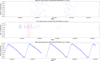 |
Fig. 1 Visualization of the difference between sparse and dense sampling of photometric light curves. We chose a classical Cepheid for this comparison. OGLE-GD-CEP-0044 is a relatively bright Cepheid with a period of 5.09 days. The upper graph shows OGLE-IV data for a 3-year-long observation window that has 130 data points. The middle graph shows observational data from the ZTF survey, also in a 3-year-long observational window with 119 data points. The third graph shows a 21.77-day-long observation from the TESS mission. The light curve contains 14 898 measurements. The time span covered by the TESS observations is presented in the middle graph by two vertical dashed lines. |
2 Data
Ground-based sky-survey programmes often produce sparse data with gaps due to observational seasons, the lunar phase, and diurnal variations. This presents many difficulties in the data-processing of periodic variable stars because their light-curve coverage is much sparser than data generated by dedicated space photometric telescopes, as shown in Figure 1. To obtain well-sampled light curves, the usual method for periodic variable stars (pulsators or eclipsing binaries) is to phase-fold the light curves. In this way, we can reveal characteristic curve shapes (Fig. 2) that are specific to the different variable star types.
To simulate the processing and sampling of future LSST data, we used synthetic data from the Extended LSST Astronomical Time-Series Classification Challenge (ELAsTiCC) (Narayan & ELAsTiCC Team 2023) dataset in our first experiments. The main purpose of this dataset was not to provide light curves for periodic variable stars, however, but to create and test end-to-end real-time pipelines for time-domain science in general, the ELAsTiCC simulated light curves still contain LSST-like light variations in six bands (ugrizY) for some variable star types, for instance, classical Cepheids or RR Lyrae stars. After some promising results, the further analysis showed that while the light-curve shapes and periods seem realistic, the generation of the light curves was not based on physical grounds, that is, it did not obey theoretical or observed trends and correlations among the observables. Hence, ELAsTiCC periodic variable star light curves were not adequate for our purposes (our training sets were always based on observed light curves and thus contain any astrophysics-based correlations), we decided to switch to ZTF observations because they are very similar in structure to those obtained with LSST. As ZTF is a pure sky-survey project, its database only contains observational data, but no cross-match between other catalogues is available for a given object. To be able to work with its data, first we had to cross-match ZTF objects with other catalogues to identify variable stars.
We used the ZTF data release 171. In the next subsection, we explain how we handled the collected dataset.
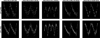 |
Fig. 2 Example gallery of the phase-folded light curve images. The five columns represent the five main variable star types that were used in this research: Classical Cepheids, δ Scuti stars, eclipsing binaries, RR Lyrae stars, and Type-II Cepheids. The top row shows g-band data, and the bottom row shows r-band data of the given example of variable star type. |
2.1 Cross-match between databases
The 51-inch (1.3 m) Warsaw University Telescope used in the OGLE sky survey program is located at the Las Campanas Observatory, Chile. This survey collects information from four different sky areas, the Galactic bulge (BLG), Galactic disk (GD), the Large Magellanic Cloud (LMC), and the Small Magellanic Cloud (SMC).
We used the OGLE-IV collection of variable stars, and we only focused on the first two observational fields, the bulge and the Galactic disk.
The ZTF at the Palomar Observatory uses the 48-inch (1.2 m) telescope to scan the entire north sky every two days in three passbands: g, r, and i. Although the telescope is located in the northern hemisphere, the overlap with the southern observatories is sufficiently large, for example, with OGLE (above a declination of −28 degrees). As our team is highly experienced with the latter and we also used OGLE variable stars to train our machine-learning algorithms (see Papers I and II), we decided to cross-match OGLE data with those from ZTF. This cross-match would clearly not contain all pulsating variable stars from the OGLE catalogue, but it was large enough to start the work.
Five different major variable star types were selected that already have sufficient data for this project. We knew that at least several hundred unique stars are needed for a well-sampled training dataset, and we were aware that data augmentation and synthetic light-curve generation is also needed. The number of selected variables per type and sub-type of star is presented in Table 1.
As Wilson & Naylor (2022) and others pointed out on numerous occasions, LSST will have such crowded fields that the standard cross-matching algorithms will fail. For us, who would like to gather information from multiple catalogues, the source identification is crucial. With the help and advice of Wilson & Naylor (priv. communication), we started to cross-match pulsating variable stars and eclipsing binaries. As the LSST point sources in the brightness range between the LSST saturation limit and the Gaia limiting magnitude will be cross-matched with the Gaia catalogue2, Gaia DR3 was used as a starting point for comparing the other two databases. First, we cross-matched the OGLE-IV catalogue with Gaia, and after this, we compared Gaia with ZTF data using a probabilistic approach. The last step was to merge the results and create the final dataset.
The details of the cross-matching side project will be published in a forthcoming paper because they are beyond the scope of this work. In the following, we only give a brief overview of the process.
The light-gathering capabilities and limiting magnitudes of these three instruments are fortunately very similar, and the crowding problem is therefore less severe when they are compared. We had to take the various passbands of the surveys into account, however. Every star from OGLE is measured in the Johnson-Cousins UBVRI photometric system (Bessell 1990), mainly in the I filter, but most stars also have V measurements. Gaia uses its unique G passband, which is operated over a much wider wavelength range, but the narrower Gaia BP and Gaia RP magnitudes are also available in many cases. Finally, the instrument of ZTF is equipped with yet another filter set, namely SDSS-like g, r, and i (Fukugita et al. 1996).
For efficient Gaia queries, the entire Gaia source and var_summary tables were downloaded, and a database was created from them on the HUN-REN Cloud (Héder et al. 2022). The database is based on the latest version of MySQL (Oracle 2025). During the cross-match process, the source positions and brightness were taken into account, and the nearest-neighbour method was used with additional matching parameters. The possible matches were categorised by the separation and the similarity of the magnitude information. For the latter, we compared the OGLE I passband with Gaia RP mean magnitudes (when available). Gaia RP covers a similar but wider wavelength range as the I passband. Despite the similarities, we used a 1.0 magnitude difference limit for the comparison. According to preliminary statistics, OGLE-IV has very precise coordinates. The average separation between OGLE and Gaia is less than 0.5 arcseconds, and we therefore used 1 arcsecond as the separation limit.
The matches were sorted into four categories: the source received score 3 when the separation and the brightness difference were smaller than the limit. Score 2 meant that the star was within the separation limit and a Gaia RP magnitude was available, but the magnitude difference was greater than the threshold. Sources received score 1 when no Gaia RP magnitudes were available, but the separation of the stars was within the set limit. OGLE stars absent from the Gaia DR3 catalogue received score 0. These stars are usually very faint, and are for example δ Scuti stars.
In the vast majority of cases, only one source matched in a given field. In other cases, when we had to deal with more than one candidate sources, the closer separation won. A few sources in question had to be reviewed by eye. In this way, we assembled a very well matched list of stars.
Stars in the ZTF sky survey are observed in g, r, and i filters. They receive a different objectid in each filter and in each observational field. They were therefore treated as separate objects, and the cross-match process was run for all filters separately. Because the i filter data are mostly only available for private projects, are not public, and the available observations are very sparse, we decided the use only the g and r filters. Our team does not work using the various ZTF alert systems, for which a given variable source receives a single ID (alert id). We used the ZTF17 database, which uses a different ID (ztf objectid). Unfortunately, these identifiers are not connected. They can only be determined in an additional cross-match, which is time-consuming and not practical. We downloaded the entire ZTF DR17 database instead and searched for and filtered our sources out.
For the cross-matching, we used a similar method as before. The sky survey website3 offers a multiple-object query, which outputs a list of objects based on the nearest-neighbour method. Because the search radius has a wider cone of 5 arcseconds, this contains much inappropriate data and therefore needs further filtering, but it is very useful in the sense that we did not have to query the whole database. Unfortunately, the SDSS g and r filters do not resemble the Gaia BP or RP magnitudes nor the OGLE-IV Johnson–Cousins I or V filters. We therefore compared the brightnesses with a slightly larger margin of error of 1.5 magnitudes.
Periodic variable stars and eclipsing binaries.
Success rate of period calculations using single-band data.
3 Preprocessing the data
3.1 Data selection and augmentation
The main goal of our team is to create methods for the classification of periodic variable stars in the LSST database. After the cross-match process was completed, we used the collected ZTF data as LSST proxy data. It is still uncertain that the periods will be calculated in the alert systems of LSST, and we therefore decided to do this in this project ourselves. The period was calculated for every star in every filter. With this information, we were able to phase-fold the raw observational g- and r-band observational data. These in most cases quite distinctive light curves with the additional period information can be separated into known variable star types. The phase-folded light curves were stored as 128x128 pixel, 1-bit images, with black background and white plotted dots. For additional information on the procedure of creating the images of the light curves, we refer to Paper I.
Data augmentation (Shorten & Khoshgoftaar 2019) was necessary because of the difference of an order of magnitude in the number of representatives falling into the given variable star classes. On the one hand, as shown in Table 1, the limited overlap of the observed sky areas means that there are, for example, fewer Classical (571 unique sources) and Type II Cepheids (568 unique sources) than δ Scuti (6882 unique sources) or RR Lyrae stars (25 702 unique sources). On the other hand, there are significant differences in the intrinsic occurrence rates of certain variable types, and also in their detection efficiencies. This number of difference, the so-called data augmentation problem, made the generation of synthetic data crucial. Synthetic phase-folded light curves were generated in the same way as described in Paper II. After the process, we had 4 500 light curves in the g and r filters from five different variable star types: classical Cepheids, δ Scutis, eclipsing binaries, RR Lyrae stars, and Type II Cepheids. We had 45 000 light curves in total.
3.2 Calculating the single-band period
The periods were calculated for every variable star in this sample for the g and r filters using the MultiHarmonicFitter function of the seismolab software package (Bódi 2024). This analysis was particularly important for us because it allowed us to test how reliably we would be able to calculate the period of variable stars for these sparse data in the first few years of the upcoming LSST survey. As we will have very few data points per year (70–80 on average) and per filter (10–15 per filter annually), we were able to test how our method evolved from one year to the next. Therefore, we calculated the periods for 1-, 2-, 3-, and 5-year-long data segments per variable star type and compared the results to the known periods from the OGLE-IV database.
During this calculation process, our first criterion was the number of collected data points in the given observational window. Based on preliminary tests and our expertise, 20 data points were defined as the minimum required to be able to calculate periods for most of the variable star types. Because of the different period information and the poorly sampled data, it was obvious that we will need a much longer observational time base for some of the stars. Every star (in the g and r filters) was flagged when the first criterion was not met.
The second criterion was a comparison of the calculated period with the ground-truth data from the OGLE-IV catalogue. For stars for which very many measurements were collected (first criterion met), but the period calculation was not precise enough and exceeded a difference of 15% compared to the OGLE-IV periods, the frequency calculation boundaries were fine-tuned based on the ground-truth data. The parameters of the MultiHarmonicFitter function minimum_frequency and maximum_frequency were changed and the periods were searched within these new intervals. In this way, we obtained a success rate for the period calculation. The aggregated result is listed in Table 2. Based on these results, we will have reliable period information for the mentioned variable star types (except for the longest-period eclipsing binaries) after three years of continuous LSST operation.
3.3 Calculating the multi-band period
For variable star data that were collected by ground-based observations similar to OGLE, ZTF, and especially LSST, which have a very poor sampling, finding and calculating the correct period is a particularly difficult task. Instead of the methods used previously, new algorithms are therefore needed that make better use of the data collected by the LSST in six different filters and allow for so-called multi-band period searches (e.g., VanderPlas & Ivezić 2015) when they are used together.
Similar to other research groups, for example Di Criscienzo et al. (2023) or Huijse et al. (2018), our team is interested in using data that were collected with multiple filters to calculate periods, thereby somewhat offsetting the problems arising from poor sampling. The main topic of our paper was not to test or develop methods for calculating periods, however, partly because they were already available in the OGLE-IV database, but calculating periods using single filters or multi-band methods is important, and we therefore also ran the latter for different time windows (1, 2, 3, and 5 years). For the multi-band period calculation, the LombScargleMultiband class was used from the Astropy (Astropy Collaboration 2022) package. After multiple runs, we decided to use 20 points for the samples_per_peak and 25 points for the maximum_frequency parameters.
For comparison, the multi-band method performed better for shorter time windows (1 and 2 years). The results are significantly better for the Classical Cepheids and the Type-II Cepheids, which have longer (some days) periods. The algorithm performed worse for the δ Scuti stars and eclipsing binaries, which have very short periods, shorter than a fraction of a day in most cases. For the eclipsing binaries, we not only confirmed whether the period was correct, but also if the result we obtained was half or twice the original period. We accepted these values and those that differed slightly (5% at most) from the baseline value.
The aggregated result is listed in Table 3. Based on these results, we find that multi-band period calculations have much potential when the observational window is long enough for a sufficient number of observations in every filter.
Success rate of period calculations using the multi-band Lomb-Scargle method.
3.4 Training, validation, and test dataset
During the pre-processing phase, the dataset mentioned in the previous subsection was divided into two non-overlapping parts, one part for the training and validation (4 000 stars) and the other part for testing purposes (500 stars). The training-validation dataset later was again separated into two parts with a 0.7 ratio: 70% was used for training, and 30% was used for the validation. We ensured that all variable star types were equally represented in the training and validation samples with either original or augmented light curves.
3.5 Variable star classes and labels
A supervised neural network method was used during the training-validation phase. This type of neural network needs a well-labelled dataset in which every category has a unique identification. In our previous work, we were able to train the network using not only the main variable star types, but also the sub-types, with outstanding accuracy (Paper II). In this work, however, we were only able to use samples from the OGLE-IV galactic disc (GD) and galactic bulge (BLG) fields because neither the LMC nor the SMC is visible in ZTF. Some pulsating variable star types that were mentioned in our previous papers, for example anomalous Cepheids, are therefore missing from the current dataset. Moreover, some variable star classes unfortunately had only a few targets in the overlapping catalogues. If we had broken them down into further groups, we would have had even fewer data to work with. We therefore decided only train the main variable star types in this experiment, Classical Cepheids, δ Scuti stars, eclipsing binaries, RR Lyrae stars, and Type II Cepheids.
4 Neural network
The architecture of the neural network contains two main parts (see Figure 3 and Table 4). The first part is a convolutional neural network (CNN). The g- and r-filter phase-folded light curves are the image-based inputs for two separate CNNs that are concatenated in the end. The second part of the network handles the numerical input, in this case, the periods. Both parts perform the classification independently and estimate the variable star class. Both are concatenated in the end, and a final classification is made for the type.
This paper is not intended to describe the different types of neural network layers. Only the basic structure is described below (we refer to Paper I, which contains these descriptions). The network was developed using the Keras API built over TensorFlow (Abadi et al. 2015), an open source platform for machine learning. Every code was written in Python.
4.1 Light-curve (image) classification
The classification of the image-based data was performed by two identical CNNs (as we described in the previous subsection), which can be separated into four different parts. The first part consists of two convolutional layers with 7×7 and 5×5 convolutional windows, followed by a dropout and a pooling layer. The purpose of this first section is the extraction of low-level features and the resizing of input images.
The high-level features were extracted in the following parts, separated into three blocks. The first two contained the same architecture, with three convolutional layers using 3×3 convolutional windows, ending with one dropout and one pooling layer. The last block contained two convolutional layers with the usual dropout and pooling layers. After this, we applied a flatten layer to create a usable input for the fully connected and the softmax layers.
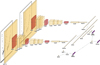 |
Fig. 3 Architecture of our neural network, which can classify image-based phase-folded light curves in multiple (in this case, two) passbands with additional numerical input (in this case, the periods) measured in each passband. From left to right: Two light curves for the same variable star in two different passbands, g and r, are the image inputs of the neural network. These images are processed by two identical CNNs and are then concatenated together for a classification based on the image (light curve) information alone. The additional numerical inputs are the passband-dependent periods of the given variable star, which also processed in a much simpler fully connected neural network. These two inputs and their results are concatenated in the end to make the final classification result. |
Hyperparameters of the neural network.
4.2 Numerical data
The period of the variable stars served as numerical inputs, basically, floating point numbers, in the network. Periods calculated from the g and r band light curves were handled by two fully connected layers with a softmax activation function. The output of this layer is the classification based on periods alone.
4.3 Concatenating the outputs
The image and the numerical data have the same number of output classes, and we therefore concatenated them and used the result as a new input for a further joint classification. The two (or more) concatenated outputs were fed as a single input to a fully connected layer with 64 units, the output of which was sent to a softmax dense layer that performed the final classification.
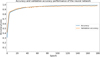 |
Fig. 4 History curves of the neural network show the evolution of the training and validation accuracy during the training and validation phases. |
4.4 Training optimization and early stopping
In our recent works, we performed thorough tests for the best-fit hyperparameters. The Adam (adaptive moment estimation) optimizer with a learning rate of 0.00025 was used, similar to our previous papers. The batch value of 32 was used during the training and validation process. This value controls the number of training examples in one forward/backward pass; lower values require less memory, and these so-called mini batches typically train the network faster. With this parameter, it took 405 iterations to complete one training epoch. Table 4 lists the hyperparameters of the neural network.
To avoid overfitting, we applied an EarlyStopping callback during training, which monitors the change of the validation loss value. We set the min_delta and patience values to 10−4 and 19, respectively. These values were chosen during the hyperparameter optimization.
4.5 Randomized phase test
At the referee’s request, we performed a test to randomize the phase. The suggestion was that in the case of variable stars, no external information should be introduced, for example by ensuring that the maximum of the pulsating variable stars or the minimum of the eclipsing binaries fell at the zero phase, which is the general procedure in period determination methods. During the test, we randomized the phase of the maximum/minimum value in the 0–1 interval, thereby filtering out this bias. This involved regenerating all light curves and rerunning the training and testing algorithms. According to our test, we were able to reproduce the results that were obtained without the phase-randomizing step, which means that our algorithm did not learn the phase information, but instead works based on the light-curve shape. We attach the confusion matrix in the appendix (see Figure A.1).
5 Results
In the following, we evaluate the training performance of the neural network and present our classification results on the test sample of the variable stars.
5.1 Training performance
Figure 4 shows the evolution of the training and validation accuracy during the training and validation phase. Related to this, Figure 5 shows the change in the loss during this phase in detail. For the training and testing process, we used a GPU-accelerated computer containing NVidia GeForce RTX 2080 Ti GPU cards. The TensorFlow environment we used is fully GPU-supported, and the computation therefore benefits fully from the available GPUs.
The training phase took about 170 epochs, and one epoch lasted for 6 seconds. The whole training and validation phase took about 17 minutes. For the training, we used 14 000 stars, and for the validation 6 000, stars were included in the g and r filters.
Examination of the curves shows that the neural network performed well, and except for some subtle anomalies, the loss curves decreased and the accuracy curves increased continuously. By the 170th epoch, the early stopping terminated the learning. As the training and validation metrics evolved at the same pace, the network did not overfit.
 |
Fig. 5 History curves of the neural network show the evolution of the training and validation loss during the training and validation phases. |
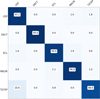 |
Fig. 6 Confusion matrix of the testing phase, which shows the performance of our neural network using ZTF data. The inputs were phase-folded light curves in two ZTF passbands (g and r) and the given stellar periods. |
5.2 Testing performance and classification of light curves
After the training and validation phase were completed, we used the selected test dataset and started the testing phase. The classification of the complete test dataset (2500 variable stars) took 0.7 seconds. Figure 6 shows the result of the process. The confusion matrix clearly shows that the classification accuracy is above 94% for four variable star classes (for three classes, it is above 98%). Only Type II Cepheids have a slightly lower classification accuracy result, but it is still around 90%. The meaning of these definitions were detailed in our previous paper (see (Szklenár et al. 2020)).
The results of two related groups, Classical Cepheids and Type-II Cepheids, are worth reporting in more detail. The other three types, the δ Scuti stars, the eclipsing binaries, and the RR Lyrae stars, have an almost negligible classification error. For the Classical Cepheids, 5.2% of the test stars were misclassified by the neural network, the majority of which (4.4%) are classified as Type-II Cepheids.
The classification result is worse for the Type-II Cepheids. 8.4% of these stars were identified as Classical Cepheid and 2% as eclipsing binary.
As the classification error was slightly higher for these two types, we selected the stars that were misclassified from the tested stars and studied their light curves manually. The problem lies in the precision of the classification, not in the labels.
 |
Fig. 7 Test results using only one passband. The g-filter data are presented on the left, and the r filter data are shown on the right. Periods were used as additional numerical inputs. The accuracy of the latter is close to those obtained with multiple passbands, but the accuracy of the classification of Cepheids is significantly worse. |
5.3 Results for one passband
As our previously published works have shown, the classification of periodic variable stars with only one passband observations can achieve accurate results, even more so with additional numerical data (e.g. periods). We ran single-filter tests with the neural network to compare the performance with multiple passband results. Figure 7 shows the classification result of the test sample when only one filter was used. Similarly to the architecture of the multiple passband neural network, the phase-folded light-curve images and the periods as numerical data were used as inputs in this case. The comparison of this figure to the previous results shows that it is worth combining data from different passbands to improve the accuracy of the most dubious classes.
6 Summary and conclusions
We have trained and tested a neural network that can classify light curves obtained in multiple colour filters using their associated period as numerical data. During the pre-processing, we selected variable stars from the data collected by the ZTF sky survey programme that are also included in the OGLE-IV database. This choice was made because the latter contains a well-categorised reliably classified dataset. Since ZTF data are similar to the upcoming LSST observations in sampling, sky coverage, and passbands, they demonstrated that we can classify periodic variable stars observed in multiple filters, and also the efficiency with which we can do this.
In order to cross-match OGLE-IV periodic variable stars with the public ZTF object catalogue, we used the Gaia astrometric measurements. During this process, we involved a probabilistic comparison of the target coordinates and brightness. When Gaia RP magnitudes were available, we compared them with the OGLE-IV I magnitudes and ruled out every source that did not match our criteria.
The ZTF observes in g, r, and i filters, but the latter is only partially available in the public data and was therefore omitted. We only used the g and r filters. The ZTF website4 provides a multiple object search feature, where the coordinates were given as input, and we received a filtered list of sources based on the nearest-neighbour method. This was further filtered based on the previously matched Gaia coordinates and brightness data.
Since the chosen different variable star classes, Classical Cepheids, δ Scuti stars, eclipsing binaries, RR Lyrae stars, and Type II Cepheids, are represented in vastly different numbers in our sample, it was necessary to create synthetic data. After the data augmentation process, we had 4500 light curves of each variably type in the g and r filters for training and testing purposes.
To classify variable stars observed by the LSST, it is essential to know the source period, and we therefore decided to determine this numerical parameter from the ZTF data, even though the period was known from OGLE. In addition to calculating the period, we ran statistics to determine after how many years we would be able to calculate the period of different types of variable stars. Since both the ZTF and the future LSST will have very few data points per year and per band, for some variable types (e.g. multi-periodic delta Scuti stars, double- or triple-mode Cepheids, or long-period Mira semi-regular variable stars), it will be particularly difficult not only to determine the period, but also to generate phase-folded light curves at the beginning of the 10-year survey. For the newly discovered variable stars, our statistics shows that we need three years of data at least to classify most of the pulsating and eclipsing variable stars. The situation will be much better for the periodic variables discovered previously, however, especially for those with a securely determined period value.
Before we trained a neural network using multiple colour filters, we also constructed a neural network to classify light curves with only one filter and its associated periods to determine the change in efficiency when only one filter is available. Our preliminary results showed an accuracy of 73–100% with the g filter and an accuracy of 87–99% with the r filter.
In contrast, the neural network that used the two filters together showed a classification probability of between 90–100%, which can be considered a significant improvement in the neural network training process and in the classification accuracy compared to the one-filter approach.
When we started this project, the actual ZTF data release was DR15, from which our dataset was upgraded to DR17. As almost 2 years have passed since then, and the latest release is DR23, which contains many more data. Our tests will continue with these and even newer ones, and hopefully, we can extend the research to three different filters (g, r, and i) as well. This would be very useful before the start of LSST, which will observe in six different filters (u, g, r, i, z, and Y).
Processing the large amount of data collected by the LSST using six filters poses a huge challenge. The quality of the data generated during the 10-year-long sky survey programme is well demonstrated by the LSST data preview 1 (DP1) data package released after the first submission of our paper. The DP1 cadence in selected sky areas mimics the 10-year LSST survey cadence (Malanchev et al. 2025). Malanchev et al. published ugrizy light curves of several known variable (pulsating and eclipsing) stars. The next step in our research will also go in these directions to benefit from multi-band LSST observations by using multi-band period search methods, and by developing corresponding neural networks.
Data availability
The architecture of the neural network and the output weight file can be downloaded from our research team’s website, using the following link: https://konkoly.hu/KIK/data_en.html#ML.
Acknowledgements
This project is funded by the SNN-147362 grant of the Hungarian National Research, Development and Innovation Office. This project is also supported by the SeismoLab project which is funded by the KKP-137523 grant and the Elvonal (Forefront) Research Excellence Program of the National Research, Development and Innovation Office. On behalf of the Varclass -- Variable star classification project we are grateful for the possibility to use HUN-REN Cloud (see (Héder et al. 2022); https://science-cloud.hu/) which helped us to achieve the results published in this paper. This work has made use of data from the European Space Agency (ESA) mission Gaia (https://www.cosmos.esa.int/gaia), processed by the Gaia Data Processing and Analysis Consortium (DPAC, https://www.cosmos.esa.int/web/gaia/dpac/consortium). Funding for the DPAC has been provided by national institutions, in particular the institutions participating in the Gaia Multilateral Agreement. Based on observations obtained with the Samuel Oschin Telescope 48-inch and the 60-inch Telescope at the Palomar Observatory as part of the Zwicky Transient Facility project. ZTF is supported by the National Science Foundation under Grants No. AST-1440341 and AST-2034437 and a collaboration including current partners Caltech, IPAC, the Weizmann Institute for Science, the Oskar Klein Center at Stockholm University, the University of Maryland, Deutsches Elektronen-Synchrotron and Humboldt University, the TANGO Consortium of Taiwan, the University of Wisconsin at Milwaukee, Trinity College Dublin, Lawrence Livermore National Laboratories, IN2P3, University of Warwick, Ruhr University Bochum, Northwestern University and former partners the University of Washington, Los Alamos National Laboratories, and Lawrence Berkeley National Laboratories. Operations are conducted by COO, IPAC, and UW. Last but not least, we would like to thank our colleague, László Molnár, for his professional advice, which contributed to the completion of our article.
References
- Abadi, M., Agarwal, A., Barham, P., et al. 2015, TensorFlow: Large-Scale Machine Learning on Heterogeneous Systems, software available from https://www.tensorflow.org/ [Google Scholar]
- Astropy Collaboration (Price-Whelan, A. M., et al.) 2022, ApJ, 935, 167 [NASA ADS] [CrossRef] [Google Scholar]
- Becker, I., Protopapas, P., Catelan, M., & Pichara, K. 2025, A&A, 694, A183 [NASA ADS] [CrossRef] [EDP Sciences] [Google Scholar]
- Bellm, E. C., Kulkarni, S. R., Graham, M. J., et al. 2019, PASP, 131, 018002 [Google Scholar]
- Bessell, M. S. 1990, PASP, 102, 1181 [NASA ADS] [CrossRef] [Google Scholar]
- Bódi, A. 2024, J. Open Source Softw., 9, 7118 [Google Scholar]
- Borucki, W. J. 2016, Rep. Progr. Phys., 79, 036901 [Google Scholar]
- Chiong, G., Becker, I., & Protopapas, P. 2025, A&A, submitted [arXiv:2506.11637] [Google Scholar]
- Dattilo, A., Vanderburg, A., Shallue, C. J., et al. 2019, AJ, 157, 169 [NASA ADS] [CrossRef] [Google Scholar]
- Dawson, J. M., Davis, T. A., Gomez, E. L., et al. 2020, MNRAS, 491, 2506 [Google Scholar]
- Di Criscienzo, M., Leccia, S., Braga, V., et al. 2023, ApJS, 265, 41 [NASA ADS] [CrossRef] [Google Scholar]
- Fukugita, M., Ichikawa, T., Gunn, J. E., et al. 1996, AJ, 111, 1748 [Google Scholar]
- Gaia Collaboration (Vallenari, A., et al.) 2023, A&A, 674, A1 [NASA ADS] [CrossRef] [EDP Sciences] [Google Scholar]
- George, D., Shen, H., & Huerta, E. A. 2018, Phys. Rev. D, 97, 101501 [Google Scholar]
- Gieseke, F., Bloemen, S., van den Bogaard, C., et al. 2017, MNRAS, 472, 3101 [NASA ADS] [CrossRef] [Google Scholar]
- Héder, M., Rigó, E., Medgyesi, D., et al. 2022, Inform. Társadalom, 22, 128 [Google Scholar]
- Hon, M., Stello, D., & Zinn, J. C. 2018, ApJ, 859, 64 [NASA ADS] [CrossRef] [Google Scholar]
- Huijse, P., Estévez, P. A., Förster, F., et al. 2018, ApJS, 236, 12 [NASA ADS] [CrossRef] [Google Scholar]
- Ivezić, Ž., Kahn, S. M., Tyson, J. A., et al. 2019, ApJ, 873, 111 [Google Scholar]
- LeCun, Y., Haffner, P., Bottou, L., & Bengio, Y. 1999, in Feature Grouping, ed. D. Forsyth (Springer) [Google Scholar]
- Malanchev, K., DeLucchi, M., Caplar, N., et al. 2025, arXiv e-prints [arXiv:2506.23955] [Google Scholar]
- Masci, F. J., Laher, R. R., Rusholme, B., et al. 2018, PASP, 131, 018003 [Google Scholar]
- Möller, A., & de Boissière, T. 2020, MNRAS, 491, 4277 [CrossRef] [Google Scholar]
- Moreno-Cartagena, D., Protopapas, P., Cabrera-Vives, G., et al. 2025, A&A, 703, A41 [NASA ADS] [CrossRef] [EDP Sciences] [Google Scholar]
- Narayan, G., & ELAsTiCC Team. 2023, in American Astronomical Society Meeting Abstracts, 241, American Astronomical Society Meeting Abstracts, 117.01 [Google Scholar]
- Oracle. 2025, MySQL, https://www.mysql.com/ [Google Scholar]
- Osborn, H. P., Ansdell, M., Ioannou, Y., et al. 2020, A&A, 633, A53 [NASA ADS] [CrossRef] [EDP Sciences] [Google Scholar]
- Pawlak, M., Soszyński, I., Udalski, A., et al. 2016, Acta Astron., 66, 421 [Google Scholar]
- Pérez-Galarce, F., Martínez-Palomera, J., Pichara, K., Huijse, P., & Catelan, M. 2025, MNRAS, 540, 3263 [Google Scholar]
- Pietrukowicz, P., Soszyński, I., Netzel, H., et al. 2020, Acta Astron., 70, 241 [Google Scholar]
- Ricker, G. R., Winn, J. N., Vanderspek, R., et al. 2015, J. Astron. Telesc. Instrum. Syst., 1, 014003 [Google Scholar]
- Shorten, C., & Khoshgoftaar, T. M. 2019, J. Big Data, 6, 60 [CrossRef] [Google Scholar]
- Soszyński, I., Udalski, A., Szymański, M. K., et al. 2014, Acta Astron., 64, 177 [NASA ADS] [Google Scholar]
- Soszyński, I., Udalski, A., Szymański, M. K., et al. 2017, Acta Astron., 67, 297 [NASA ADS] [Google Scholar]
- Soszyński, I., Udalski, A., Wrona, M., et al. 2019, Acta Astron., 69, 321 [Google Scholar]
- Soszyński, I., Udalski, A., Szymański, M. K., et al. 2020, Acta Astron., 70, 101 [Google Scholar]
- Soszyński, I., Pietrukowicz, P., Skowron, J., et al. 2021, Acta Astron., 71, 189 [Google Scholar]
- Szklenár, T., Bódi, A., Tarczay-Nehéz, D., et al. 2020, ApJ, 897, L12 [CrossRef] [Google Scholar]
- Szklenár, T., Bódi, A., Tarczay-Nehéz, D., et al. 2022, ApJ, 938, 37 [CrossRef] [Google Scholar]
- Udalski, A., Szymański, M. K., & Szymański, G. 2015, Acta Astron., 65, 1 [NASA ADS] [Google Scholar]
- Udalski, A., Soszyński, I., Pietrukowicz, P., et al. 2018, Acta Astron., 68, 315 [Google Scholar]
- Ulaş, B., Szklenár, T., & Szabó, R. 2025, A&A, 695, A81 [NASA ADS] [CrossRef] [EDP Sciences] [Google Scholar]
- VanderPlas, J. T., & Ivezić, Ž. 2015, ApJ, 812, 18 [Google Scholar]
- Wilson, T. J., & Naylor, T. 2022, in The 21st Cambridge Workshop on Cool Stars, Stellar Systems, and the Sun, https://doi.org/10.5281/zenodo.7464177 [Google Scholar]
Science Validation of LSST Data Release Processing – http://pstn-039.lsst.io
ZTF catalog search: https://irsa.ipac.caltech.edu/Missions/ztf.html
ZTF website: https://www.ztf.caltech.edu/index.html
Appendix A Randomized phase test
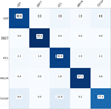 |
Fig. A.1 At the referee’s request, we performed a test how our neural network architecture would perform with randomized phase. For this test we created a completely new training and testing dataset where the phase of the maximum/minimum value in the 0–1 interval was randomized. In this case the light curve minima of the eclipsing binaries and the maxima of the pulsating variable stars should not have any external information. Our results show that our neural network does not learn the phase information, only the light curve shape. |
All Tables
All Figures
|
Fig. 1 Visualization of the difference between sparse and dense sampling of photometric light curves. We chose a classical Cepheid for this comparison. OGLE-GD-CEP-0044 is a relatively bright Cepheid with a period of 5.09 days. The upper graph shows OGLE-IV data for a 3-year-long observation window that has 130 data points. The middle graph shows observational data from the ZTF survey, also in a 3-year-long observational window with 119 data points. The third graph shows a 21.77-day-long observation from the TESS mission. The light curve contains 14 898 measurements. The time span covered by the TESS observations is presented in the middle graph by two vertical dashed lines. |
| In the text | |
|
Fig. 2 Example gallery of the phase-folded light curve images. The five columns represent the five main variable star types that were used in this research: Classical Cepheids, δ Scuti stars, eclipsing binaries, RR Lyrae stars, and Type-II Cepheids. The top row shows g-band data, and the bottom row shows r-band data of the given example of variable star type. |
| In the text | |
|
Fig. 3 Architecture of our neural network, which can classify image-based phase-folded light curves in multiple (in this case, two) passbands with additional numerical input (in this case, the periods) measured in each passband. From left to right: Two light curves for the same variable star in two different passbands, g and r, are the image inputs of the neural network. These images are processed by two identical CNNs and are then concatenated together for a classification based on the image (light curve) information alone. The additional numerical inputs are the passband-dependent periods of the given variable star, which also processed in a much simpler fully connected neural network. These two inputs and their results are concatenated in the end to make the final classification result. |
| In the text | |
|
Fig. 4 History curves of the neural network show the evolution of the training and validation accuracy during the training and validation phases. |
| In the text | |
|
Fig. 5 History curves of the neural network show the evolution of the training and validation loss during the training and validation phases. |
| In the text | |
|
Fig. 6 Confusion matrix of the testing phase, which shows the performance of our neural network using ZTF data. The inputs were phase-folded light curves in two ZTF passbands (g and r) and the given stellar periods. |
| In the text | |
|
Fig. 7 Test results using only one passband. The g-filter data are presented on the left, and the r filter data are shown on the right. Periods were used as additional numerical inputs. The accuracy of the latter is close to those obtained with multiple passbands, but the accuracy of the classification of Cepheids is significantly worse. |
| In the text | |
|
Fig. A.1 At the referee’s request, we performed a test how our neural network architecture would perform with randomized phase. For this test we created a completely new training and testing dataset where the phase of the maximum/minimum value in the 0–1 interval was randomized. In this case the light curve minima of the eclipsing binaries and the maxima of the pulsating variable stars should not have any external information. Our results show that our neural network does not learn the phase information, only the light curve shape. |
| In the text | |
Current usage metrics show cumulative count of Article Views (full-text article views including HTML views, PDF and ePub downloads, according to the available data) and Abstracts Views on Vision4Press platform.
Data correspond to usage on the plateform after 2015. The current usage metrics is available 48-96 hours after online publication and is updated daily on week days.
Initial download of the metrics may take a while.