| Issue |
A&A
Volume 706, February 2026
|
|
|---|---|---|
| Article Number | A194 | |
| Number of page(s) | 15 | |
| Section | Extragalactic astronomy | |
| DOI | https://doi.org/10.1051/0004-6361/202556280 | |
| Published online | 13 February 2026 | |
Galaxy interactions in void substructures: Morphology and stellar populations of two triplets from CAVITY
1
Departamento de Física Teórica y del Cosmos, Universidad de Granada (UGR) Avenida de la Fuente Nueva s/n C.P. 18071 Granada, Spain
2
Instituto de Física, Universidade Federal do Rio Grande do Sul (UFRGS) Av. Bento Goncalves 9500 Porto Alegre RS, Brazil
3
Instituto Universitario Carlos I de Física Teórica y Computacional, Universidad de Granada 18071 Granada, Spain
4
Instituto de Matemática Estatística e Física, Universidade Federal do Rio Grande (IMEF – FURG) Av Itália s/n Rio Grande RS, Brazil
5
Centre for Astrophysics Research, University of Hertfordshire College Lane Hatfield AL10 9AB, UK
★ Corresponding author: This email address is being protected from spambots. You need JavaScript enabled to view it.
Received:
7
July
2025
Accepted:
28
November
2025
Abstract
Context. Cosmic voids, vast, underdense regions of the Universe, serve as unique laboratories for studying galaxy evolution in isolation. Within these voids, galaxy triplets, rare systems of three close galaxies, provide crucial insights into how local interactions shape stellar populations and morphology in the absence of strong environmental perturbations.
Aims. We investigate the spatially resolved stellar populations, morphologies, mass assembly histories, and dynamical properties of six galaxies from the Calar Alto Void Integral-field Treasury surveY (CAVITY). These galaxies reside in two void triplet systems, CAVITY5273X and VGS31.
Methods. We employed integral field unit (IFU) spectroscopy combined with full spectral fitting using the FADO code, which simultaneously models stellar and nebular emission. We derived maps of stellar ages, metallicities, and star formation rates, applying the integrated nested Laplace approximation (inla) for spatial reconstruction. Morphological analysis was conducted using morfometryka, and emission-line diagnostics were employed to assess ionization mechanisms. Mass-assembly functions were computed to reveal the stellar mass evolution of the galaxies. We also compared stellar metallicities and stellar masses to the mass-metallicity relation (MMR) for void galaxies.
Results. The two triplets exhibit distinct evolutionary pathways. CAVITY52731 is a massive, quenched active galactic nucleus host, while young stellar populations and recent star formation dominate its companions and the three members of VGS31. The galaxies in both triplets show diverse mass assembly functions, with some building most of their stellar mass early and others exhibiting significant late-time star formation. All five star-forming galaxies present rapid mass growth in the last 2 Gyr (by a factor of ∼1.4 − 4). Morphological analysis in the g band of the DESI Legacy Survey and in the literature reveals widespread disturbances, including tidal tails, arcs, and asymmetries, indicating active dynamical evolution. Although galaxies in CAVITY5273X follow the expected MMR for voids, those in VGS31 deviate significantly, likely due to filamentary accretion and recent interactions.
Conclusions. Our results demonstrate that even in the most underdense regions of the cosmic web, galaxies can experience dynamic evolution driven by local interactions and minor mergers. Void triplets challenge the traditional view of voids as passive environments and highlight the importance of small-scale structures in shaping galaxy properties.
Key words: galaxies: evolution / galaxies: interactions / galaxies: stellar content
© The Authors 2026
 Open Access article, published by EDP Sciences, under the terms of the Creative Commons Attribution License (https://creativecommons.org/licenses/by/4.0), which permits unrestricted use, distribution, and reproduction in any medium, provided the original work is properly cited.
This article is published in open access under the Subscribe to Open model. This email address is being protected from spambots. You need JavaScript enabled to view it. to support open access publication.
1. Introduction
Cosmic voids are vast, underdense regions that occupy most of the volume of the Universe, playing a crucial role in the formation and dynamical evolution of large-scale structures in the cosmic web (Bothun et al. 1992; Colless et al. 2003; Tegmark et al. 2004; van de Weygaert et al. 2016; Moews et al. 2021; Vallés-Pérez et al. 2021; Zhang et al. 2022; Bermejo et al. 2024). These voids are enormous regions that usually span 20−50 h−1 Mpc in size (El-Ad & Piran 1997; Hoyle & Vogeley 2002; Plionis & Basilakos 2002; Hoyle & Vogeley 2004; Conroy et al. 2005; Sutter et al. 2012), are surrounded by denser filaments and walls of galaxies, and have very low densities of matter, down to ≲20% of the mean cosmic density (van de Weygaert & Platen 2011; Pan et al. 2012).
The voids originate from the underdensities of the primordial Universe (Planck Collaboration I 2020), in the region where the expansion overcame the gravitational attraction of the matter. Such regions are where cosmic expansion occurs with the highest intensity, and as voids expand, matter is pulled toward their borders by gravity and squeezed between them, and sheets and filaments form the boundaries of voids (van de Weygaert & Platen 2011). Numerical simulations support models in which smaller-scale voids disappear into large ones (Dubinski et al. 1993; van de Weygaert & van Kampen 1993; Colberg et al. 2005; Sheth & van de Weygaert 2004) and the density in the voids evolves to constant values in the local Universe, with a higher galaxy density profile toward their boundaries (van de Weygaert & Platen 2011).
Cosmological voids are exceptional laboratories for studying the evolution of galaxies with minimal influence from environmental effects, such as ram pressure stripping, mergers, tidal forces, thermal evaporation, and harassment, among others. In addition, the dark matter content in such regions is believed to be lower, and they expand faster than the mean of the cosmic web (Biswas et al. 2010; van de Weygaert & Platen 2011; Hamaus et al. 2016). For instance, mature voids emulate a low-density Friedmann-Lemaître-Robertson-Walker universe (Goldberg & Vogeley 2004; Lavaux & Wandelt 2012; Hamaus et al. 2014), and dark matter halos in voids were formed later than their counterparts in overdense regions (Yang et al. 2012; Tojeiro et al. 2017; Wechsler & Tinker 2018).
The galaxy populations inside voids differ in various aspects from non-void galaxies, due to their different dynamical histories. For example, when compared to galaxies in filaments and walls, some studies find that void galaxies are, on average, younger, bluer, richer in H I, less metal-enriched, and smaller, and have lower stellar masses, higher specific star formation rates (sSFRs) and later morphological types (Peebles 2001; Rojas et al. 2004; Croton et al. 2005; Rojas et al. 2005; Hoyle et al. 2012; Kreckel et al. 2012; Beygu et al. 2016; Douglass et al. 2018; Florez et al. 2021; Pandey et al. 2021; Rodríguez Medrano et al. 2022; Rosas-Guevara et al. 2022; Argudo-Fernández et al. 2024; Curtis et al. 2024). However, other works indicate that void and non-void galaxies are very similar in properties, such as stellar masses, gas content, star formation rates (SFRs), chemical abundances, dark matter profiles, and metallicities (Szomoru et al. 1996; Patiri et al. 2006; Moorman et al. 2014; Liu et al. 2015; Douglass & Vogeley 2017; Douglass et al. 2019; Wegner et al. 2019; Domínguez-Gómez et al. 2022). Thus, the ways in which void and non-void galaxies differ from each other are still poorly understood.
Recent results obtained with the Calar Alto Void Integral-field Treasury surveY (CAVITY, Pérez et al. 2024), Domínguez-Gómez et al. (2023a) show that the stellar mass assembly of void galaxies is slower than in denser environments. They find a bimodality in star formation histories (SFHs) in all environments (voids, filaments, walls, and clusters). One group formed less than 21.4% of its stellar mass ∼12.5 Gyr ago, while the other formed higher fractions of its stellar mass at the same time. For both cases, the SFHs in voids are the slowest. Also, Domínguez-Gómez et al. (2023b) find that galaxies in voids exhibit slightly lower central stellar metallicities (∼0.1 dex) than those in filaments and walls, and much lower (∼0.4 dex) than those in clusters. These differences are more pronounced in low-mass galaxies (≲ 109.25 M⊙), galaxies with long-timescale SFHs, and spiral and blue galaxies. Additionally, Conrado et al. (2024) find that void galaxies have a slightly higher half-light radius (HLR), a lower stellar mass surface density, younger ages across all morphological types, and a slightly elevated SFR and sSFR (only significant enough for Sas). Their analysis also indicates that void galaxies undergo a more gradual evolution, especially in their outer regions, with a more pronounced effect for low-mass galaxies.
Voids are dynamic and evolving systems (Courtois et al. 2023). They asymptotically evolve to empty and structureless regions as the space expands and the gravitational force of the clusters and surrounding filaments and walls pull the galaxies and dark matter halos toward the void outskirts (van de Weygaert & Platen 2011). However, in the local Universe, the voids are still not devoid of internal structure. As those voids expand and merge hierarchically, structures such as diffuse filaments and groups of galaxies may remain inside those voids (Szomoru et al. 1996; El-Ad & Piran 1997; Hoyle & Vogeley 2004; Kreckel et al. 2012; Beygu et al. 2013; Alpaslan et al. 2014). Some of the remaining substructures we find in voids are galaxy triplets, which are the simplest type of galaxy groups formed by three galaxies (Karachentseva et al. 1979; Karachentseva & Karachentsev 2000; Elyiv et al. 2009; Makarov & Karachentsev 2009). Such systems located in voids are very scarce, and there is no vast literature on them. Isolated galaxy triplets represent only 3% of galaxies with magnitudes in the r band of 11 ≤ mr ≤ 15.7 at low redshifts 0.005 ≤ z ≤ 0.08 (Argudo-Fernández et al. 2015). Also, the majority of triplets are located in the outer parts of filaments, walls, and clusters, instead of voids. Some important catalogs of triplets in the literature are Karachentseva et al. (1979), Trofimov & Chernin (1995), O’Mill et al. (2012), and Argudo-Fernández et al. (2015).
Most galaxy triplets exhibit signs of a long dynamical evolution whereby the system is embedded in a common dark matter halo, and the member galaxies present similar properties (Chernin et al. 2000; Hernández-Toledo et al. 2011; Duplancic et al. 2013; Feng et al. 2016; Emel’yanov et al. 2016). In that sense, they are much closer to compact groups (CGs; Duplancic et al. 2015; Costa-Duarte et al. 2016), which are formed by four galaxies or more. Duplancic et al. (2013) found that galaxies in triplets have colors, SFRs, and stellar populations similar to CGs. Also regarding stellar populations, Vásquez-Bustos et al. (2023) find that there is no dominant type of galaxy in isolated triplets in terms of global colors and the SFR.
An additional interest in void galaxies is that we can properly investigate the local environmental influence of the neighboring galaxies on each other and discard the interference of large-scale structures (clusters and groups) dynamics. Argudo-Fernández et al. (2015) found no difference in the interaction of large-scale environments with isolated galaxies, isolated pairs, and isolated triplets. This suggests that both have common origins and the differences in observational properties are due to differences in their local environments and dynamics.
This work characterizes the stellar populations of six galaxies belonging to two void triplet systems. We performed spatially resolved stellar population synthesis (SPS) on the integral field unit (IFU) data obtained by CAVITY. To perform the synthesis, we used the code FADO (Gomes & Papaderos 2017) and the front-end software URUTAU.
The structure of this paper is organized as follows. Section 2 explains the data and methodologies used in this work. In Sect. 3 we present our results. In Sect. 4 we discuss their implications, followed by our conclusions in Sect. 5. Throughout this work we use the following cosmology: H0 = 67 km s−1 Mpc−1, ΩM = 0.3, and ΩΛ = 0.7 (Kozmanyan et al. 2019).
2. Data
2.1. CAVITY spectroscopy
The data used in this work were obtained from CAVITY (Pérez et al. 2024). It is a legacy survey conducted at the Calar Alto Observatory, aiming to obtain spatially resolved spectroscopy of approximately 300 void galaxies in the local Universe. These galaxies are distributed across 15 cosmological voids, with redshifts in the range of 0.005 < z < 0.05, and have absolute r-band magnitudes between −21.5 and −17.0. The first data release was done with 100 galaxies (García-Benito et al. 2024), though none of the objects studied in this work are in DR1.
Observations were carried out using the integral field Potsdam Multi-Aperture Spectrograph (PMAS; Roth et al. 2005), mounted on the 3.5m telescope at the Hispanic Astronomical Center in Andalusia (CAHA), operating in PPaK mode (Kelz et al. 2006). PPaK consists of over 300 fibers, each with a diameter of 2.68 arcsec, arranged to cover a hexagonal field of view (FoV) of 74 × 64 arcsec2 with a filling factor of approximately 60%. The V500 grating was used, offering a spectral range of 3475−7300 Å and a spectral resolution of λ/Δλ = 850 at 5000 Å, corresponding to a full width at half maximum (FWHM) of roughly 6 Å. The cubes were reduced and calibrated through the standard CAVITY data reduction pipeline and they were corrected for galactic extinction during this procedure (for more details, see García-Benito et al. 2024).
2.2. Imaging
In Sect. 4.4 we use broad band images in order to perform the morphological study of our targets. We use the images of the g band from the Dark Energy Spectroscopic Instrument (DESI) Legacy Survey (Dey et al. 2019). This survey uses as its main instrument the Dark Energy Camera (DECam) in the Blanco Telescope in Chile, in addition to the Mosaic3 Camera in the Mayall Telescope in EUA. Both instruments have pixels with an angular size of 0.262 arcsec, and an angular resolution between ∼1 and ∼1.5 arcsec, depending on the band. The g band, by being the bluer filter in the gri system, provides some of the best evidence of the asymmetries in the young populations in the galaxies.
2.3. Sample
The subjects of this study are two galaxy triplet systems located in distinct cosmological voids. They were the first triplets observed by the survey. Figure 1 shows RGB images of the triplets obtained from Pan-STARRS (Chambers et al. 2016). We refer to these systems as CAVITY5273X and VGS31. These two specific systems were selected because they were the only triplets with all three galaxies observed by CAVITY’s IFU.
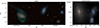 |
Fig. 1. RGB images of the two triplets taken from DESI Legacy Survey. The left panel shows the VGS31 triplet, with VGS31a in the center, VGS31b to its southeast, and VGS31c to its west. The right panel shows CAVITY5273X, with CAVITY52731 to the east, CAVITY52732 to its west, and CAVITY52733 to its southwest. |
There is no detailed literature available on CAVITY5273X. This system comprises a larger, redder galaxy (i.e., CAVITY52731) accompanied by two smaller, bluer companions to its west (i.e., CAVITY52732) and southwest (i.e., CAVITY52732). All three galaxies exhibit some degree of morphological asymmetry in the light, as is discussed further in Sect. 4.4. For example, CAVITY52732 features two tidal tails.
VGS31, on the other hand, is also part of the Void Galaxy Survey (VGS, van de Weygaert et al. 2011) and has been studied previously by Beygu et al. (2013), who found it to be embedded in an H I filament. This makes VGS31 an example of a filamentary structure within a void, suggesting that its constituent galaxies may be undergoing active growth. The system is composed of a central galaxy (i.e., VGS31a), a similarly sized galaxy to its east (i.e., VGS31b), and a smaller one to its west (i.e., VGS31c). All galaxies in the system show asymmetric features in the images, particularly VGS31b, which exhibits a tidal tail to the north and a ring-like arc to the south – likely the result of a minor merger (Beygu et al. 2013). Table 1 summarizes basic previously known properties of these galaxies.
Previously measured basic information about the galaxies.
3. Methodology
3.1. Spectral fitting
In order to implement the SPS in the CAVITY datacubes, we used the nonparametric code FADO (Fitting Analysis using Differential evolution Optimisation; Gomes & Papaderos 2017). To achieve the best-fitting solution, FADO employs a genetic differential evolution optimization (DEO) algorithm in which each candidate model – defined by stellar population fractions, extinction, and kinematics – is treated as an individual within a population that evolves through mutation and recombination. At each generation, the fittest models are selected, ensuring convergence toward solutions that simultaneously reproduce the stellar continuum and the nebular emission.
The additional constraint of the nebular emission was computed from the fluxes of various emission lines (Hα, Hβ, [N II], [S II], [O III], etc.). This constraint is critical for the synthesis of star-forming galaxies (Cardoso et al. 2019), since it enables the computation of nebular spectra in addition to the stellar ones. The software computes the number of ionizing photons required to produce the observed fluxes of the main emission lines, especially the Balmer lines, as hydrogen is ionized by photons with wavelengths shorter than 912 Å, which are emitted by hot, massive young stars (t < 20 Myr). This way, it estimates the necessary fraction of young stellar populations to account for the observed ionization.
To run a SPS code, it is necessary to supply a base of simple stellar populations (SSPs). In this work, we use a base comprising 68 SSPs from Bruzual & Charlot (2003, hereafter BC03), with a Chabrier (2003) initial mass function (IMF), and lower and upper stellar mass limits of 0.1 M⊙ and 100 M⊙, respectively. Our choice of BC03 is due to its ability to consistently extend into the ionizing UV domain (λ < 912 Å), which is required by FADO’s self-consistent modeling of stellar and nebular emission. Among the available models, there is only one that covers the ionizing UV emission and has a spectral resolution in the optical comparable to the data in the optical: the BC03 (FWHM ≈ 3 Å). The BC03 models also have their limitations, particularly for the intermediate-age range, which gets under-sampled as a result of insufficient TP-AGB modelling (Riffel et al. 2015; Lu et al. 2025). However, such subrepresentation affects the NIR spectral range more than the optical. The models from Maraston (2005) also cover the ionizing UV domain, but have a poorer spectral resolution in the optical (FWHM ≈ 10 − 20 Å). Although newer versions of these models present higher resolutions, such as Maraston & Strömbäck (2011), they do not cover the ionizing domain, reaching down to 1000 Å.
However, it is unnecessary to use the entire SSP library from BC03, since many models are redundant for synthesis purposes. Simple stellar populations with similar ages and metallicities often have nearly indistinguishable spectra, particularly for older populations (t > 5 Gyr), and the inclusion of observational noise further reduces their discriminability. Moreover, using an excessively large base greatly increases computational time without significant improvements in fitting accuracy. Instead, it is best to select a representative subset covering different age ranges. We followed the methodology described in Dametto et al. (2014) and also applied in Azevedo et al. (2023) for BC03, selecting a base of 68 SSPs with 17 representative ages (t = 1.00, 2.09, 3.02, 5.01, 10.00, 25.12, 50.00, 101.50, 321.00, 508.80, 718.70 Myr and 1.02, 2.00, 3.00, 5.00, 10.00, 13.00 Gyr) and four metallicities ( ), which have seven representative ages for young populations (t < 100 Myr), seven representative ages for intermediate populations (100 Myr < t < 5 Gyr), and three for old populations (t ≥ 5 Gyr).
A challenge when applying SPS to datacubes is that the synthesis codes are designed for single spectra. Therefore, one must extract the spectrum from each spaxel, apply the synthesis individually, and then store the results, indexing them back to their corresponding spaxels. Fortunately, there is a front-end pipeline called URUTAU1 (Riffel et al. 2023) that automates all these steps and, additionally, writes the synthesis results into new extensions of the original datacube. URUTAU operates through modules dedicated to each processing step, such as extraction, dereddening, synthesis, and result reading, as well as offering extra features. However, the original modules were developed specifically for use with STARLIGHT (Cid Fernandes et al. 2005), which functions quite differently from FADO. Thus, we developed new modules to run FADO on the spectra and to parse its outputs accordingly.
3.2. Spatial reconstruction
When we implement SPS methodology on IFU data, the SPS needs to be applied to each spaxel independently. This can generate abrupt variations in the values of a given measurement of two neighboring pixels. For instance, a pixel can have a low mean age and its neighbor can have a high mean age, which is not physically accurate. Smoother gradients are expected for this kind of extended source (González-Gaitán et al. 2019).
In order to avoid such cases and produce smoother morphological maps with a mathematically robust methodology, we made use of the integrated nested Laplace approximation (inla). It is an alternative method to Markov chain Monte Carlo for fast Bayesian inference. Its mathematical foundations and applications to IFU data from the CALIFA and PISCO surveys are presented in González-Gaitán et al. (2019). Azevedo et al. (2023) also applied the method to spatially resolved data from the MUSE spectrograph. INLA is highly efficient at both reconstructing data from extended sources with missing pixels and smoothing data by considering spatial correlations. Large variations between neighboring pixels for physical quantities such as stellar ages or metallicities may be unphysical. In this context, the method accounts for spatial correlations between adjacent pixels to reconstruct a more physically consistent map. There is a comprehensive R library for implementing INLA.
In this work, we used it on 2D maps, such as those shown in Sect. 3.4. It also acts as a way to correlate the results of the SPS analysis from individual spaxels, which are treated independently in our synthesis, but in reality are part of the same extended source. Figure 2 presents an example of ⟨log t⟩L maps before and after applying INLA to the map.
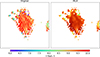 |
Fig. 2. Comparison of the ⟨log t⟩L map for the galaxy CAVITY52731 before (left) and after (right) applying INLA. |
3.3. Signal-to-noise ratio
The reliability of a SPS depends on the signal-to-noise ratio (S/N) of the spectra. Figure 3 shows the S/N contours overlaid on the luminosity maps of each galaxy. The S/N values were computed in the featureless continuum wavelength window from 4000 to 4060 Å. This wavelength range is the same as that used to normalize the spectra during the SPS process, and it was chosen to maintain consistency.
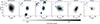 |
Fig. 3. Maps of luminosities of the galaxies, with the colored lines indicating different contours of S/N. The red contour is for S/N ≥ 10, the green for 5, and the blue for 3. The S/Ns were computed in the wavelength interval of 4000−4060 Å. |
It is also close to the lower wavelength limit of our observed data. The blue end of the spectrum is significantly noisier than the red end in our data, with uncertainties in the 4000−4060 Å range reaching values up to ten times higher than those at the opposite end. However, this region is also the most relevant for SPS, since the slope of the NUV and blue continuum contains the most prominent differences between different stellar populations, especially the youngest ones.
Therefore, the most reliable synthesis results correspond to spaxels with S/N ≥ 10, which generally excludes the outer regions of our galaxies. All the spaxels that appear in Fig. 3 were used in the analysis, but it is important to keep in mind that the results on the outskirts of the galaxies are less reliable.
3.4. Spectral fits outputs
A SPS code provides a series of different quantities for each spectrum, both directly or that can be easily obtained from its results, such as mean stellar ages and metallicities, stellar masses, stellar and nebular radial velocities and velocity dispersions, SFRs, stellar and nebular extinctions, among many others (Cid Fernandes et al. 2005; Gomes & Papaderos 2017). FADO, for instance, by dealing with nebular emission physics, also returns fluxes, equivalent widths, rotation velocity, and velocity dispersion for various emission lines, in addition to the number of ionizing photons for hydrogen and helium.
The mean stellar ages are defined in two ways (Cid Fernandes et al. 2005; Gomes & Papaderos 2017). The mean age weighted by light can be expressed as
 (1)
(1)
Meanwhile, the mean age weighted by mass is expressed as
 (2)
(2)
where tj is the age of the j-th SSP from the base measured in years, xj is the fraction with which it contributes to light, μj is the fraction with which it contributes to mass, and N★ is the number of SSPs in the base. Similarly, the mean stellar metallicities are defined as
 (3)
(3)
 (4)
(4)
where Zj is the metallicity of the j-th SSP. The fraction of light or mass represented by each SSP is provided in what we call population vectors.
Another important measurement we can make using the population vectors is the SFR. We can compute it through the equation (Riffel et al. 2021, and references therein)
 (5)
(5)
where j refers to the j-th SSP in the base, and M★c is the total mass converted to stars in the time interval Δt. It is worth highlighting that the stellar mass converted to stars is different than the mass present available in stars. The present stellar mass takes into account the mass expelled by the stars during their evolution, while the other represents all the mass collapsed into stars in a certain time epoch. FADO computes the total M★c and we can then use the coefficients, μj, to find the mass converted into stars in a given time.
As we have those measurements for each pixel of the galaxy, we can investigate the spatial distribution of the characteristics of the stellar populations and of the gas in the galaxies. We plot 2D morphological maps of some of the main quantities; that is, the integrated luminosity of the spectrum, the nebular extinction, mean stellar ages and metallicities weighted both by light and mass, and the SFRs computed through the population vector. Figure 4 shows the maps for the galaxy CAVITY52731.
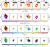 |
Fig. 4. 2D maps of luminosities, SFR surface densities, mean stellar ages and metallicities, for all six galaxies in our sample. |
3.5. Integrated spectra
Besides the methodology explained in previous sections for implementing the SPS in the spectra of each spaxel, we also computed the integrated spectra for each galaxy to measure global properties more easily and reliably. We summed all spectra for which the SPS were implemented, after the quality filters and URUTAU implementation described in Sect. 3.1. This way, we guaranteed a good S/N in the spectra (S/N > 30 in 4000−4060 Å). Then we implemented FADO with them and could derive global measurements from the galaxies, such as total stellar mass and global mean stellar ages. Some measurements based on the synthesis of the integrated spectra are shown in Table 2. Results shown in Table 3 and Figs. 6 and 7 were also obtained through the integrated spectra. This approach also allows for direct comparisons with the sample in Costa-Duarte et al. (2016), hereafter CD16.
Stellar population characteristics computed through FADO with the integrated spectra.
Emission lines fluxes and ratios, and BPT and WHAN classification computed through FADO with the integrated spectra (fluxes are in units of ×1016 erg/s/cm2).
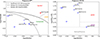 |
Fig. 6. BPT diagram (left) and WHAN diagram (right) for the galaxies in this work, obtained from the integrated spectra. |
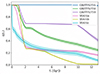 |
Fig. 7. Stellar mass assembly function for the galaxies in triplets. The functions are the mean of the 100 different curves generated with Monte Carlo after perturbing the spectra and applying FADO in each of them. The shaded regions represent the error of the mean. These functions were obtained from the integrated spectra. |
CD16 analyses the stellar populations and ionization sources of 80 isolated galaxy triplets in the redshift range 0.04 ≥ z ≥ 0.1, applying the SPS code STARLIGHT in SDSS spectra. Although it uses single fiber spectra of the central parts, rather than IFU data, its approach is similar to ours when implementing SPS. And since it studies a large sample, it represents a good comparison base for this work. One caveat, however, is that the galaxies in that sample are at higher redshifts than the ones that are the focus of this work.
4. Results and discussion
4.1. Emission lines
The gas of five of the galaxies that we investigate is ionized by recent star formation, as we verify in the maps of BPT classification shown in Fig. 5. The only exception is CAVITY52731, the most massive in its system, which has its nebular emission powered mostly by Seyfert and composite sources. In fact, its main power source is classified as a Seyfert by the BPT diagram and as a weak active galactic nucleus (AGN) by the WHAN diagram, as is shown in Fig. 6 (unlike the maps of BPT classification for each spaxel, these diagrams were made using the integrated spectra). It is also the galaxy with the oldest stellar populations, being the only one in our sample with ⟨log t⟩L higher than 9. CAVITY52731 most likely is a massive (M★ ≈ 1011 M⊙) quenched galaxy that hosts an AGN, while the rest are less massive (M★ < 1010 M⊙) active star-forming ones. Information about the emission lines and BPT and WHAN classifications of the sample is shown in Table 3.
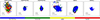 |
Fig. 5. Maps of BPT classification for the galaxies. Blue is for star-forming spectra, green for composite, yellow for LINER-like emission, and red for Seyfert. |
According to CD16, most galaxies in isolated triplets are classified as AGN or passive in the WHAN diagram, even considering only the least massive systems, with only about 8% of the galaxies being dominated by star formation. However, this result may also be biased by the fact that the spectra in CD16 are obtained with single fiber, covering the central parts of the galaxies. This way, galaxies that might be dominated by star formation in their outskirts may not be classified as mainly powered by star formation. Nevertheless, galaxies in our study are dominated by star formation, which might indicate they are among the rarest in terms of the ionization source. Also, VGS31c has a specially low value of log(N II/Hα).
4.2. Mass assembly
Except for CAVITY52731, all the other objects have stellar populations younger than 25 Myr that contribute significantly to the light (10%−40%) but represent less than 1% of the mass. We also computed the stellar mass assembly function (Asari et al. 2007) for each galaxy, which is defined as
 (6)
(6)
This is a cumulative function that grows from 0 to 1, starting at the oldest SSP in the spectral base and tracking what fraction of the stellar mass was due to stars formed up to a given look-back time. The computed curves are presented in Fig. 7.
Here we also applied a simple Monte Carlo method, by perturbing the spectra of the galaxies 100 times, considering for each wavelength a Gaussian distribution with σ equal to its error. Then we ran FADO in each new spectrum to reobtain the necessary quantities, such as total mass and population vectors. Then we had, for each galaxy, the mean of the 100 generated curves and the error of the mean.
Domínguez-Gómez et al. (2023b) found that the SFHs at early times describe a bimodal distribution in the three large-scale environments (voids, filaments, walls and clusters), which allow us to classify the SFHs into two types: short-timescale SFH (ST-SFH) galaxies that formed a large fraction of their stellar mass (27% on average) ∼12.5 Gyr ago, and long-timescale SFH (LT-SFH) galaxies that formed a lower fraction of their stellar mass (< 21.4%) than the ST-SFH galaxies 12.5 Gyr ago, but formed stars more uniformly over time. We can verify, based on Fig. 7, that the three galaxies in VGS31 and CAVITY52732 have LT-SFH, while CAVITY52731 and CAVITY52733 have ST-SFH.
We verified that CAVITY52731 formed most of its mass at early epochs of the Universe (t > 1010 yr), while the others have significant star formation at more recent times. All the others present a rapid increase in their mass in the last 2 Gyr. Before that, their star formation was more continuous. This is in agreement with the previous results (see Figs. 5 and 6) and evidence that only CAVITY52731 is a passive galaxy in those systems. Although CAVITY52733 is classified as ST-SFH by the criteria of the mass formed 12.5 Gyr ago, the increase in the SFR at earlier times is more similar to the behavior of an LT-SFH. It is not totally in accordance with the general behavior found for cluster galaxies (and other environments as well), which assemble on average 30% of their mass at early times and decrease their SFR later in their lives. This may be indicative of a more complex evolutionary path than non-triplet galaxies. In fact, Domínguez-Gómez et al. (2023b) presents the mass assembly function for the galaxies in CAVITY, grouping by LT-SFH and ST-SFH, revealing their general behavior, and their functions are smooth through time, as well as the functions for two examples of CAVITY galaxies shown in the same work. Those facts might indicate that the great increase in SFR at late times, as we see in our sample, is not common for void galaxies.
The mass assembly function for CAVITY52731 shows no star formation in the last 10 Gyr, evidencing a fast mass assembly common for massive and quiescent galaxies. However, we must consider that the spectra of old SSPs with the same metallicity are nearly indistinguishable. For ages on the gigayear scale, the spectra show little evolution with time. In our base, we chose only three ages to represent the old populations: 5, 10, and 13 Gyr (for ages lower than 1 Gyr, the age resolution of the base is much higher). That means that the galaxy could, in fact, have star formation at times between those large intervals, but the SPS codes do not differentiate them much. In fact, verifying the population vectors for the various results in the Monte Carlo for CAVITY52731, there is in fact populations with t★ = 5 Gyr or t★ = 1 Gyr, although they never represent more than 0.2% of the mass. We also detect populations with t★ = 5 Myr that are responsible for less than 5% of the light.
We also leveraged the Monte Carlo implementation in the SPS to compute the stellar masses of the galaxies, which are shown in Table 2. Both triplets are among the least massive triplets, being below the 33.3% percentile of the stellar mass distribution from CD16 (log M★ < 11.52). This may already be expected due to the fact that galaxies in voids are, in general, less massive than galaxies in filaments, walls, and clusters. VGS31 has a total stellar mass of log M★ = 9.86 and CAVITY5273X has log M★ = 10.99. In that sense, VGS31 is a particularly unique triplet, since it is formed by three dwarf galaxies. The least massive systems in CD16 have log M★(M⊙)∼11.0. The uncertainties in the masses are quite small (up to ∼0.1 dex in the logarithmic space), except for VGS31c, which has an uncertainty of ∼0.5.
4.3. Mass-metallicity relation
Finally, we compared the stellar metallicities of the six galaxies to the mass-metallicity relation (MMR) extracted from Domínguez-Gómez et al. (2023a) for void galaxies. In that work, the stellar metallicities were obtained through a nonparametric full spectral fitting analysis applied to SDSS-DR7 spectra using the PPXF (Cappellari 2017) and STECKMAP (Ocvirk et al. 2006a,b) codes. They modeled the spectra in the 3750−5450 Å range, combining single stellar population (SSP) templates from the E-MILES library and assuming a Kroupa IMF. The stellar line-of-sight velocity distribution and gas emission lines were first fit with PPXF; the emission was subtracted, and the stellar population parameters were then derived with STECKMAP assuming the fixed kinematics from PPXF. The SSP metallicities cover 2.27 ≤ [M/H]≤0.40 dex, where [M/H]=log(Z/Z⊙).
Domínguez-Gómez et al. (2023a) computes the stellar metallicity in the galaxies within their central 3 arcsec. The sample used to represent the void galaxies was the CAVITY sample as well, and since each fiber of PPAK has a diameter of 2.7 arcsec, we used the spectrum of the central spaxel in the galaxy to derive the metallicity. Following Domínguez-Gómez et al. (2023a), we computed the metallicities as
![Mathematical equation: $$ \begin{aligned}{[\mathrm{M/H}]}_M = \sum _{j = 1}^{N_{\star }} \mu _j \log (Z_j/Z_{\odot }), \end{aligned} $$](/articles/aa/full_html/2026/02/aa56280-25/aa56280-25-eq8.gif) (7)
(7)
where Zj is the metallicity of the j-th SSP in the base and μj is the mass fraction of that population.
The MMR is shown in Fig. 8. The galaxies in CAVITY5273X follow the MMR quite well, being inside one standard deviation (σ) of the distribution. On the other hand, VGS31a and VGS31b are outliers, as they have [M/H]M outside 1σ of the distribution. This could be due to their more complex evolutionary path, since they are embedded in an H I filament and are interacting. Besides the fact that all of them are dwarf galaxies, VGS31a shows signatures of a past merger, and VGS31a shows indications of tidal interactions with the other galaxy or accretion from filamentary material (Beygu et al. 2013). In fact, all three galaxies could accrete filamentary material, which, together with the interactions, might trigger or keep star formation. This process enriches the gas and stars subsequently formed, along with the fact that the gas in filaments is generally less metal-rich compared to the galaxies.
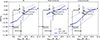 |
Fig. 8. Mass-metallicity relation for the galaxies in our sample. In blue we have the MMR for void galaxies, taken from Domínguez-Gómez et al. (2023a). The dashed lines are the mean values, the shaded regions are the error of the mean, and the dotted lines mark the 1σ distribution in metallicity. The MMR is shown for three different samples: all void galaxies (from CAVITY), ST-SFH void galaxies, and LT-SFH void galaxies. The black dots indicate the masses and central metallicities of the galaxies in our sample. The points are the mean of the 100 different points generated for each galaxy with Monte Carlo after perturbing the spectra and applying FADO in each of them. The error bars indicate the standard deviation of the Monte Carlo generated sample. |
In the case of CAVITY5273X, the galaxies also seem to be interacting with one another, although we cannot be sure since we do not have more details on their dynamics. Also, it is not embedded in a filament, so it appears to be a less complex scenario, but the interactions could cause different episodes of star formation in different regions of the galaxies, which may lead to complex stellar metallicities. We also verify that metallicities can vary significantly across different locations within those galaxies, as is shown in the maps in Fig. 4, rather than analyzing only the integrated spectra.
Domínguez-Gómez et al. (2023a) derived MMRs separately for those two different SFHs (LT-SFH and ST-SFH) as well, which are also shown in Fig. 8. CAVITY52732 and CAVITY52731 fall inside the 1σ distribution for both relations, while the galaxies VGS31b and VGS31c are still outliers in both distributions.
4.4. Morphology
All galaxies in both triplets present asymmetric structures that indicate interactions. In order to complement the stellar population and ionized gas analysis performed in the previous sections, we computed a series of morphological parameters, which allowed us to better understand the structure of those objects.
Here we made use of the code MORFOMETRYKA (Ferrari et al. 2015). It consists of a standalone application to automatically perform all the structural and morphometric measurements over a galaxy image. Between them are the original and modified parameters of the concentration, asymmetry, smoothness, Gini, and M20 (CASGM) system, presented in Abraham et al. (1994, 1996), Conselice et al. (2000), Lotz et al. (2004), in addition to Sérsic indexes (Sersic 1968), and the new parameters entropy and spirality. The most recent version of MORFOMETRYKA also provides the curvature of the brightness profile with KURVATURE (Lucatelli & Ferrari 2019), which is a powerful tool for probing the presence of multiple components in galaxies.
Figure 9 shows the morphology decompositions of the galaxies in CAVITY5273X and VGS31, alongside with the models, residuals and A1 map computed by MORFOMETRYKA, as well as their luminosity profiles, and 1D and 2D Sérsic profiles. The images used are from the g band of the DESI Legacy Survey (Dey et al. 2019). A1 is measured as defined by Abraham et al. (1996), by subtracting the rotated galaxy image (Iπ) from the original galaxy image (I) within the Petrosian radius (Rp) and without subtracting the sky, following
 (8)
(8)
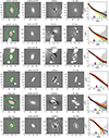 |
Fig. 9. MORFOMETRYKA output for CAVITY 52731 (upper row), CAVITY 52732 (middle), and CAVITY 52733 (lower). In the columns, from left to right: original image in g band (arcsinh scale); single Sérsic model fit and PSF (lower left insert); single Sérsic residual; asymmetry map; and brightness profile (black dots) and 1D (yellow) and 2D (red) derived Sérsic models. In the leftmost panels, the dark green line is the initial segmentation region; the neon green lines are the two Petrosian radius regions (obtained both by fitting Sérsic and by image momenta); the red line corresponds to the Sérsic Rn. In the rightmost panels, black dots and bars are measurements and associated uncertainties; the yellow line is the Sérsic fit to the 1D profile; the red line is the profile but with the parameters obtained from the image (2D) fits. |
The residuals and A1 maps evidence the asymmetry present in all galaxies in the two triplets. CAVITY52732 and VGS31b are probably the most eye-catching in the sample due to their clear disturbance. The first presents two highlighted tidal tails, one extended to the northwest and another to the southeast, and the last presents a ring-like structure to the south and a long tail to the northeast. Such features are relatively easy to identify just by looking at the RGB images of the systems. But unfortunately, such structures are mostly too faint to have sufficient S/N and be synthesized by our SPS method.
CAVITY52733 also has an extended emission to the south, and VGS31a has one to the southeast. VGS31c, being tinier, may be the most difficult one in which to identify any disturbance. The only one that seems undisturbed or mildly perturbed is CAVITY52731, maybe because the mass of its companions is too low in proportion to significantly affect the orbits of the stars, and they have not merged yet.
Regarding the surface brightness profile, we see a large-scale structure that has a convex shape in the surface brightness profile in most of the galaxies. However, MORFOMETRYKA cannot fit most of the details that stem from the irregular structure, so a more accurate profile may deviate even more than a single Sérsic component profile. The insufficiency of single-component Sérsic models to describe the surface brightness is one more piece of evidence of the disturbed morphology of those galaxies.
The only galaxy that is well represented by a 2D Sérsic model is CAVITY52731, which is a passive galaxy and dominates its system in mass. Its profile is close to an elliptical galaxy with n2D ∼ 2, although it presents an obscured stripe parallel to its semimajor axis (SMA), which resembles the extinction by the dust in a disk seen edge-on. This could indicate that this galaxy has an S0 morphology. CAVITY52732, which has two tidal tails, is relatively well modeled by a Sérsic model also with n2D ∼ 2 up to radii 0.5Rp, but presents a less concentrated brightness for larger distances. CAVITY52733 has a structure closer to a disk (n2D ∼ 1) up to radii of R ∼ 0.75Rp.
When it comes to the triplet in the filament, they seem to deviate even more than their 2D Sérsic models. The profiles for both VGS31a and VGS31c transition from a concave to a convex curve around R ∼ 0.8Rp. VGS31b, the one with an arc to the south and a long tail to the north, has a concentrated light in the center, after transitioning to a more concave curve up to R ∼ 1Rp, and after returning to a convex profile. The tail and the ring-like structures are likely caused by a past minor merger incident with a low-mass galaxy (Mihos & Hernquist 1994, 1996; Duc & Renaud 2013).
A multiwavelength study of VGS31 triplet was performed by Beygu et al. (2013), combining observations of the optical, Hα, NUV and FUV, and CO(1−0). That work finds that the tail and arc structures in VGS31b are devoid of star formation, in opposition to its central regions, which characterizes a starburst. The galaxy presents a bar, and its kinematics are indicative of fast-rotating inner structure and streaming motions. VGS31a also has disturbed internal kinematics and an enhanced SFR, which could be explained by a tidal interaction with VGS31b or by the accretion of the filamentary material. VGS31c also has an enhanced SFR and disturbed kinematics, but it is difficult to further investigate the possible scenarios because of the low S/N.
5. Summary and conclusions
In this work, we have presented a spatially resolved analysis of six galaxies in two triplets residing within cosmological voids, using integral field spectroscopy from the CAVITY survey. Our results reinforce the view that, despite the overall low-density conditions in voids, galaxies therein can exhibit rich and diverse evolutionary histories driven by internal mechanisms and local interactions. The main conclusions of our study are:
-
CAVITY52731 is markedly different from the rest of the sample, showing signs of early mass assembly, while the remaining galaxies display prominent young stellar populations and active star formation.
-
Morphological features such as tidal tails, arcs, and asymmetric light distributions are common in both triplets, indicating that galaxy interactions and minor mergers are actively shaping these systems even in void regions.
-
Emission-line diagnostics confirm that most galaxies are powered by recent star formation, with CAVITY52731 being the only exception, exhibiting AGN-like signatures in both BPT and WHAN diagrams.
-
Stellar mass assembly histories reveal that while some galaxies formed most of their mass early in the Universe’s history, others underwent significant recent star formation, reflecting diverse and nonuniversal evolutionary paths. While one of the star-forming galaxies (CAVITY52733) has an ST-SHF and the other four have an LT-SFH, all of them present accelerated mass assembly in the last 2 Gyr.
-
The stellar MMR reveals contrasting behavior between the two systems. While CAVITY5273X galaxies follow the MMR expected for void galaxies, the VGS31 galaxies appear as significant outliers, particularly in terms of metallicity. This may indicate the influence of filamentary accretion.
-
Sérsic profile fits and residuals demonstrate that most galaxies deviate significantly from regular morphologies, further confirming their disturbed nature and supporting scenarios involving interactions and accretion.
These findings emphasize that galaxy evolution in voids is not a passive process. Instead, local interactions and small-scale structures, such as triplets and filaments, play a critical role in driving stellar and morphological transformations. Furthermore, deviations from standard relations such as the MMR provide valuable insights into how environmental context can shape the chemical evolution of galaxies.
Acknowledgments
Based on observations collected at the Centro Astronómico Hispano en Andalucía (CAHA) at Calar Alto, operated jointly by Junta de Andalucía and Consejo Superior de Investigaciones Científicas (IAACSIC). The CAVITY project acknowledges financial support from projects PID2020-113689GB-I00 and PID2023-149578NB-I00, financed by MCIN/AEI/10.13039/501100011033 and FEDER/UE; from FEDER/Junta de Andalucía-Consejería de Transformación Económica, Industria, Conocimiento y Universidades/Proyecto A-FQM-510-UGR20; from grant AST22_4.4 financed by Junta de Andalucía-Consejería de Universidad, Investigación e Innovación and Gobierno de España and European Union-NextGenerationEU; and from projects P20_00334 and FQM 108 financed by the Junta de Andalucia. GMA acknowledges financial support Coordenação de Aperfeiçoamento de Pessoal de Nível Superior (CAPES Proj. 0001) and the Programa de Pós-Graduação em Física (PPGFis) at UFRGS. MAF acknowledges support from the Emergia program (EMERGIA20_38888) from Consejería de Universidad, Investigación e Innovación de la Junta de Andalucía. BB acknowledges financial support from the Grant AST22-4.4, funded by Consejería de Universidad, Investigación e Innovación and Gobierno de España and Unión Europea – NextGenerationEU, and by the research projects PID2020-113689GB-I00 and PID2023-149578NB-I00 financed by MCIN/AEI/10.13039/501100011033. BB acknowledges financial support from the Grant AST22-4.4, funded by Consejería de Universidad, Investigación e Innovación and Gobierno de España and Unión Europea – NextGenerationEU, and by the research projects PID2020-113689GB-I00 and PID2023-149578NB-I00 financed by MCIN/AEI/10.13039/501100011033. ALCS acknowledges support from FAPERGS (grants 23/2551-0001832-2 and 24/2551-0001548-5), CNPq (grants 314301/2021-6, 312940/2025-4, 445231/2024-6, and 404233/2024-4), and CAPES (grant 88887.004427/2024-00). RR acknowledges support from CNPq(445231/2024-6, 311223/2020-6, 404238/2021-1, and 310413/2025-7), FAPERGS (19/1750-2 and 24/2551-0001282-6) and CAPES(88881.109987/2025-01).
References
- Abraham, R. G., Valdes, F., Yee, H. K. C., & van den Bergh, S. 1994, ApJ, 432, 75 [NASA ADS] [CrossRef] [Google Scholar]
- Abraham, R. G., van den Bergh, S., Glazebrook, K., et al. 1996, ApJS, 107, 1 [NASA ADS] [CrossRef] [Google Scholar]
- Alpaslan, M., Robotham, A. S. G., Obreschkow, D., et al. 2014, MNRAS, 440, L106 [Google Scholar]
- Argudo-Fernández, M., Verley, S., Bergond, G., et al. 2015, A&A, 578, A110 [NASA ADS] [CrossRef] [EDP Sciences] [Google Scholar]
- Argudo-Fernández, M., Gómez Hernández, C., Verley, S., et al. 2024, A&A, 692, A258 [NASA ADS] [CrossRef] [EDP Sciences] [Google Scholar]
- Asari, N. V., Cid Fernandes, R., Stasińska, G., et al. 2007, MNRAS, 381, 263 [Google Scholar]
- Astropy Collaboration (Price-Whelan, A. M., et al.) 2022, ApJ, 935, 167 [NASA ADS] [CrossRef] [Google Scholar]
- Azevedo, G. M., Chies-Santos, A. L., Riffel, R., et al. 2023, MNRAS, 523, 4680 [NASA ADS] [CrossRef] [Google Scholar]
- Bermejo, R., Wilding, G., van de Weygaert, R., et al. 2024, MNRAS, 529, 4325 [NASA ADS] [CrossRef] [Google Scholar]
- Beygu, B., Kreckel, K., van de Weygaert, R., van der Hulst, J. M., & van Gorkom, J. H. 2013, AJ, 145, 120 [NASA ADS] [CrossRef] [Google Scholar]
- Beygu, B., Kreckel, K., van der Hulst, J. M., et al. 2016, MNRAS, 458, 394 [NASA ADS] [CrossRef] [Google Scholar]
- Bidaran, B., La Barbera, F., Pasquali, A., et al. 2023, MNRAS, 525, 4329 [NASA ADS] [CrossRef] [Google Scholar]
- Biswas, R., Alizadeh, E., & Wandelt, B. D. 2010, Phys. Rev. D, 82, 023002 [NASA ADS] [CrossRef] [Google Scholar]
- Bothun, G. D., Geller, M. J., Kurtz, M. J., Huchra, J. P., & Schild, R. E. 1992, ApJ, 395, 347 [Google Scholar]
- Bradley, L., Sipőcz, B., Robitaille, T., et al. 2020, https://doi.org/10.5281/zenodo.4044744 [Google Scholar]
- Bruzual, G., & Charlot, S. 2003, MNRAS, 344, 1000 [NASA ADS] [CrossRef] [Google Scholar]
- Cappellari, M. 2017, MNRAS, 466, 798 [Google Scholar]
- Cardoso, L. S. M., Gomes, J. M., & Papaderos, P. 2019, A&A, 622, A56 [NASA ADS] [CrossRef] [EDP Sciences] [Google Scholar]
- Chabrier, G. 2003, PASP, 115, 763 [Google Scholar]
- Chambers, K. C., Magnier, E. A., Metcalfe, N., et al. 2016, ArXiv e-prints [arXiv:1612.05560] [Google Scholar]
- Chernin, A. D., Dolgachev, V. P., & Domozhilova, L. M. 2000, MNRAS, 319, 851 [Google Scholar]
- Cid Fernandes, R., Mateus, A., Sodré, L., Stasińska, G., & Gomes, J. M. 2005, MNRAS, 358, 363 [Google Scholar]
- Colberg, J. M., Sheth, R. K., Diaferio, A., Gao, L., & Yoshida, N. 2005, MNRAS, 360, 216 [NASA ADS] [CrossRef] [Google Scholar]
- Colless, M., Peterson, B. A., Jackson, C., et al. 2003, ArXiv e-prints [arXiv:astro-ph/0306581] [Google Scholar]
- Conrado, A. M., González Delgado, R. M., García-Benito, R., et al. 2024, A&A, 687, A98 [NASA ADS] [CrossRef] [EDP Sciences] [Google Scholar]
- Conroy, C., Coil, A. L., White, M., et al. 2005, ApJ, 635, 990 [Google Scholar]
- Conselice, C. J., Bershady, M. A., & Jangren, A. 2000, ApJ, 529, 886 [NASA ADS] [CrossRef] [Google Scholar]
- Costa-Duarte, M. V., O’Mill, A. L., Duplancic, F., Sodré, L., & Lambas, D. G. 2016, MNRAS, 459, 2539 [NASA ADS] [CrossRef] [Google Scholar]
- Courtois, H. M., van de Weygaert, R., Aubert, M., et al. 2023, A&A, 673, A38 [NASA ADS] [CrossRef] [EDP Sciences] [Google Scholar]
- Croton, D. J., Farrar, G. R., Norberg, P., et al. 2005, MNRAS, 356, 1155 [NASA ADS] [CrossRef] [Google Scholar]
- Curtis, O., McDonough, B., & Brainerd, T. G. 2024, ApJ, 962, 58 [NASA ADS] [CrossRef] [Google Scholar]
- Dametto, N. Z., Riffel, R., Pastoriza, M. G., et al. 2014, MNRAS, 443, 1754 [Google Scholar]
- Dey, A., Schlegel, D. J., Lang, D., et al. 2019, AJ, 157, 168 [Google Scholar]
- Domínguez-Gómez, J., Lisenfeld, U., Pérez, I., et al. 2022, A&A, 658, A124 [NASA ADS] [CrossRef] [EDP Sciences] [Google Scholar]
- Domínguez-Gómez, J., Pérez, I., Ruiz-Lara, T., et al. 2023a, A&A, 680, A111 [NASA ADS] [CrossRef] [EDP Sciences] [Google Scholar]
- Domínguez-Gómez, J., Pérez, I., Ruiz-Lara, T., et al. 2023b, Nature, 619, 269 [CrossRef] [Google Scholar]
- Douglass, K. A., & Vogeley, M. S. 2017, ApJ, 834, 186 [Google Scholar]
- Douglass, K. A., Vogeley, M. S., & Cen, R. 2018, ApJ, 864, 144 [Google Scholar]
- Douglass, K. A., Smith, J. A., & Demina, R. 2019, ApJ, 886, 153 [Google Scholar]
- Dubinski, J., da Costa, L. N., Goldwirth, D. S., Lecar, M., & Piran, T. 1993, ApJ, 410, 458 [NASA ADS] [CrossRef] [Google Scholar]
- Duc, P.-A., & Renaud, F. 2013, Lect. Notes Phys., 861, 327 [NASA ADS] [CrossRef] [Google Scholar]
- Duplancic, F., O’Mill, A. L., Lambas, D. G., Sodré, L., & Alonso, S. 2013, MNRAS, 433, 3547 [NASA ADS] [CrossRef] [Google Scholar]
- Duplancic, F., Alonso, S., Lambas, D. G., & O’Mill, A. L. 2015, MNRAS, 447, 1399 [NASA ADS] [CrossRef] [Google Scholar]
- El-Ad, H., & Piran, T. 1997, ApJ, 491, 421 [NASA ADS] [CrossRef] [Google Scholar]
- Elyiv, A., Melnyk, O., & Vavilova, I. 2009, MNRAS, 394, 1409 [NASA ADS] [CrossRef] [Google Scholar]
- Emel’yanov, N. V., Kovalev, M. Y., & Chernin, A. D. 2016, Astron. Rep., 60, 397 [CrossRef] [Google Scholar]
- Feng, S., Shao, Z.-Y., Shen, S.-Y., et al. 2016, RAA, 16, 72 [NASA ADS] [Google Scholar]
- Ferrari, F., de Carvalho, R. R., & Trevisan, M. 2015, ApJ, 814, 55 [NASA ADS] [CrossRef] [Google Scholar]
- Florez, J., Berlind, A. A., Kannappan, S. J., et al. 2021, ApJ, 906, 97 [NASA ADS] [CrossRef] [Google Scholar]
- García-Benito, R., Jiménez, A., Sánchez-Menguiano, L., et al. 2024, A&A, 691, A161 [NASA ADS] [CrossRef] [EDP Sciences] [Google Scholar]
- Goldberg, D. M., & Vogeley, M. S. 2004, ApJ, 605, 1 [NASA ADS] [CrossRef] [Google Scholar]
- Gomes, J. M., & Papaderos, P. 2017, A&A, 603, A63 [NASA ADS] [CrossRef] [EDP Sciences] [Google Scholar]
- González-Gaitán, S., de Souza, R. S., Krone-Martins, A., et al. 2019, MNRAS, 482, 3880 [CrossRef] [Google Scholar]
- Hamaus, N., Sutter, P. M., & Wandelt, B. D. 2014, Phys. Rev. Lett., 112, 251302 [NASA ADS] [CrossRef] [Google Scholar]
- Hamaus, N., Pisani, A., Sutter, P. M., et al. 2016, Phys. Rev. Lett., 117, 091302 [NASA ADS] [CrossRef] [Google Scholar]
- Hernández-Toledo, H. M., Méndez-Hernández, H., Aceves, H., & Olguín, L. 2011, AJ, 141, 74 [CrossRef] [Google Scholar]
- Hoyle, F., & Vogeley, M. S. 2002, ApJ, 566, 641 [NASA ADS] [CrossRef] [Google Scholar]
- Hoyle, F., & Vogeley, M. S. 2004, ApJ, 607, 751 [NASA ADS] [CrossRef] [Google Scholar]
- Hoyle, F., Vogeley, M. S., & Pan, D. 2012, MNRAS, 426, 3041 [NASA ADS] [CrossRef] [Google Scholar]
- Karachentseva, V. E., & Karachentsev, I. D. 2000, ASP Conf. Ser., 209, 11 [Google Scholar]
- Karachentseva, V. E., Karachentsev, I. D., & Shcherbanovsky, A. L. 1979, Astrofizicheskie Issledovaniia Izvestiya Spetsial’noj Astrofizicheskoj Observatorii, 11, 3 [Google Scholar]
- Kelz, A., Verheijen, M. A. W., Roth, M. M., et al. 2006, PASP, 118, 129 [Google Scholar]
- Kozmanyan, A., Bourdin, H., Mazzotta, P., Rasia, E., & Sereno, M. 2019, A&A, 621, A34 [NASA ADS] [CrossRef] [EDP Sciences] [Google Scholar]
- Kreckel, K., Platen, E., Aragón-Calvo, M. A., et al. 2012, AJ, 144, 16 [Google Scholar]
- Lavaux, G., & Wandelt, B. D. 2012, ApJ, 754, 109 [NASA ADS] [CrossRef] [Google Scholar]
- Liu, C.-X., Pan, D. C., Hao, L., et al. 2015, ApJ, 810, 165 [NASA ADS] [CrossRef] [Google Scholar]
- Lotz, J. M., Primack, J., & Madau, P. 2004, AJ, 128, 163 [NASA ADS] [CrossRef] [Google Scholar]
- Lu, J., Kang, X., & Shen, S. 2025, MNRAS, 540, 1491 [Google Scholar]
- Lucatelli, G., & Ferrari, F. 2019, MNRAS, 489, 1161 [NASA ADS] [CrossRef] [Google Scholar]
- Makarov, D. I., & Karachentsev, I. D. 2009, Astrophys. Bull., 64, 24 [NASA ADS] [CrossRef] [Google Scholar]
- Maraston, C. 2005, MNRAS, 362, 799 [NASA ADS] [CrossRef] [Google Scholar]
- Maraston, C., & Strömbäck, G. 2011, MNRAS, 418, 2785 [Google Scholar]
- Mihos, J. C., & Hernquist, L. 1994, ApJ, 425, L13 [Google Scholar]
- Mihos, J. C., & Hernquist, L. 1996, ApJ, 464, 641 [Google Scholar]
- Moews, B., Schmitz, M. A., Lawler, A. J., et al. 2021, MNRAS, 500, 859 [Google Scholar]
- Moorman, C. M., Vogeley, M. S., Hoyle, F., et al. 2014, MNRAS, 444, 3559 [NASA ADS] [CrossRef] [Google Scholar]
- Ocvirk, P., Pichon, C., Lançon, A., & Thiébaut, E. 2006a, MNRAS, 365, 46 [Google Scholar]
- Ocvirk, P., Pichon, C., Lançon, A., & Thiébaut, E. 2006b, MNRAS, 365, 74 [Google Scholar]
- O’Mill, A. L., Duplancic, F., García Lambas, D., Valotto, C., & Sodré, L. 2012, MNRAS, 421, 1897 [CrossRef] [Google Scholar]
- Pan, D. C., Vogeley, M. S., Hoyle, F., Choi, Y.-Y., & Park, C. 2012, MNRAS, 421, 926 [NASA ADS] [CrossRef] [Google Scholar]
- Pandey, D., Saha, K., & Pradhan, A. C. 2021, ApJ, 919, 101 [Google Scholar]
- Patiri, S. G., Prada, F., Holtzman, J., Klypin, A., & Betancort-Rijo, J. 2006, MNRAS, 372, 1710 [NASA ADS] [CrossRef] [Google Scholar]
- Peebles, P. J. E. 2001, ApJ, 557, 495 [NASA ADS] [CrossRef] [Google Scholar]
- Pérez, I., Verley, S., Sánchez-Menguiano, L., et al. 2024, A&A, 689, A213 [NASA ADS] [CrossRef] [EDP Sciences] [Google Scholar]
- Planck Collaboration I. 2020, A&A, 641, A1 [NASA ADS] [CrossRef] [EDP Sciences] [Google Scholar]
- Plionis, M., & Basilakos, S. 2002, MNRAS, 330, 399 [NASA ADS] [CrossRef] [Google Scholar]
- Riffel, R., Pastoriza, M. G., Rodríguez-Ardila, A., et al. 2015, ASP Conf. Ser., 497, 459 [Google Scholar]
- Riffel, R., Mallmann, N. D., Ilha, G. S., et al. 2021, MNRAS, 501, 4064 [NASA ADS] [CrossRef] [Google Scholar]
- Riffel, R., Mallmann, N. D., Rembold, S. B., et al. 2023, MNRAS, 524, 5640 [NASA ADS] [CrossRef] [Google Scholar]
- Rodríguez Medrano, A. M., Paz, D. J., Stasyszyn, F. A., & Ruiz, A. N. 2022, MNRAS, 511, 2688 [Google Scholar]
- Rojas, R. R., Vogeley, M. S., Hoyle, F., & Brinkmann, J. 2004, ApJ, 617, 50 [NASA ADS] [CrossRef] [Google Scholar]
- Rojas, R. R., Vogeley, M. S., Hoyle, F., & Brinkmann, J. 2005, ApJ, 624, 571 [NASA ADS] [CrossRef] [Google Scholar]
- Rosas-Guevara, Y., Tissera, P., Lagos, C. D. P., Paillas, E., & Padilla, N. 2022, MNRAS, 517, 712 [NASA ADS] [CrossRef] [Google Scholar]
- Roth, M. M., Kelz, A., Fechner, T., et al. 2005, PASP, 117, 620 [Google Scholar]
- Sersic, J. L. 1968, Atlas de Galaxias Australes (Cordoba, Argentina: Observatorio Astronomico) [Google Scholar]
- Sheth, R. K., & van de Weygaert, R. 2004, MNRAS, 350, 517 [NASA ADS] [CrossRef] [Google Scholar]
- Sutter, P. M., Lavaux, G., Wandelt, B. D., & Weinberg, D. H. 2012, ApJ, 761, 44 [NASA ADS] [CrossRef] [Google Scholar]
- Szomoru, A., van Gorkom, J. H., Gregg, M. D., & Strauss, M. A. 1996, AJ, 111, 2150 [NASA ADS] [CrossRef] [Google Scholar]
- Tegmark, M., Blanton, M. R., Strauss, M. A., et al. 2004, ApJ, 606, 702 [Google Scholar]
- Tojeiro, R., Eardley, E., Peacock, J. A., et al. 2017, MNRAS, 470, 3720 [NASA ADS] [CrossRef] [Google Scholar]
- Trofimov, A. V., & Chernin, A. D. 1995, AZh, 72, 308 [NASA ADS] [Google Scholar]
- Vallés-Pérez, D., Quilis, V., & Planelles, S. 2021, ApJ, 920, L2 [CrossRef] [Google Scholar]
- van de Weygaert, R., & Platen, E. 2011, Int. J. Mod. Phys. Conf. Ser., 1, 41 [NASA ADS] [CrossRef] [Google Scholar]
- van de Weygaert, R., & van Kampen, E. 1993, MNRAS, 263, 481 [NASA ADS] [Google Scholar]
- van de Weygaert, R., Kreckel, K., Platen, E., et al. 2011, Astrophys. Space Sci. Proc., 27, 17 [Google Scholar]
- van de Weygaert, R., Shandarin, S., Saar, E., & Einasto, J. 2016, IAU Symp., 308 [Google Scholar]
- Vásquez-Bustos, P., Argudo-Fernandez, M., Grajales-Medina, D., Duarte Puertas, S., & Verley, S. 2023, A&A, 670, A63 [NASA ADS] [CrossRef] [EDP Sciences] [Google Scholar]
- Wechsler, R. H., & Tinker, J. L. 2018, ARA&A, 56, 435 [NASA ADS] [CrossRef] [Google Scholar]
- Wegner, G. A., Salzer, J. J., Taylor, J. M., & Hirschauer, A. S. 2019, ApJ, 883, 29 [NASA ADS] [CrossRef] [Google Scholar]
- Yang, X., Mo, H. J., van den Bosch, F. C., Zhang, Y., & Han, J. 2012, ApJ, 752, 41 [NASA ADS] [CrossRef] [Google Scholar]
- Zhang, Y., de Souza, R. S., & Chen, Y.-C. 2022, MNRAS, 517, 1197 [Google Scholar]
The code is available at: https://github.com/ndmallmann/urutau
Appendix A: Elliptical isophotes
All the galaxies in the triplets seem to have some sort of asymmetry. Still, we can fit elliptical isophotes using the Python library PHOTUTILS (Bradley et al. 2020), an ASTROPY package (Astropy Collaboration 2022) for photometry. This helps us to divide the galaxy into different regions (annuli) and analyse each one separately. We applied this methodology to the maps of the integrated fluxes of the spectra of the galaxies. Figure A.1 shows the example for the galaxy VGS31b.
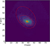 |
Fig. A.1. Map of integrated fluxes of the galaxy VGS31b. The red ellipses represent the isophotes fit with PHOTUTILS. |
By computing the mean ages and metallicities for the spaxels between two ellipses, we can obtain profiles for stellar ages and metallicities. Since the center, eccentricity, and angle of the isophotes can vary largely for the most asymmetric and clumpy galaxies. It means that the curves we compute are not exactly radial profiles, but rather measurements for regions with similar surface brightness. We choose to keep it this way because we verify that in almost all of the 6 galaxies, the ellipses change significantly as their SMA increases, and they present clear asymmetries.
Additionally to computing the mean ages or metallicities for different annuli, we perform a simple Monte Carlo method by perturbing the points 1000 times. For each point, we assume a Gaussian distribution with σ equal to its respective standard error. In the end, we have the mean of the 1000 curves generated for each galaxy, along with the error of the mean. The SMAs are normalized by the SMA of the isophote that contains 90% of the total light of the galaxy (SMA90). Figure A.2 presents the profiles for the individual galaxies in our sample, both light and mass-weighted.
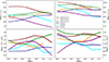 |
Fig. A.2. Mean radial profiles of < log t> L (top left), < log t> M (top right), < Z> L (bottom left), and < Z> M (bottom right). The curves were computed after performing a Monte Carlo, perturbing the mean value in each annulus 1000 times and then computing the mean of the 1000 generated curves. The shaded regions are the error of the mean. |
There is no pattern for either the mean ages or the mean stellar metallicities profiles. Regarding age, half of the galaxies present an increasing profile and the other half a decreasing profile. The curves for < log t> M are higher than the ones for < log t> L, as expected, since the mass-weighting highlights older stellar populations. In the case of CAVITY52733, the < log t> L profile is increasing, while the < log t> M starts decreasing for radii larger than ∼0.5R90. 2 galaxies present negative age profiles (VGS31b and VGS31c), which is not common. For instance, dwarf early-type galaxies of comparable mass in the Virgo cluster show age gradients always positive or nearly flat (Bidaran et al. 2023).
The mean < Z> L and < Z> M curves seem more complex. There are profiles that have a positive gradient in the inner parts of the galaxy and a negative in the outskirts. There are others that have the opposite behavior. Again, there is no clear pattern, but our sample is very small, and each galaxy may have passed through distinct evolutionary paths and had distinct SFHs.
Appendix B: Age bin maps
This section presents the age bins maps for the galaxies in our sample (Figs. B.1 and B.2). By binning the stellar populations by age, disregarding metallicities, we obtain the SFHs of the galaxies in the form of the fraction of mass (or light) enclosed in each population. We present it in a different manner, however. Instead of curves or histograms, we show 2D maps with such fractions, with each panel in the image representing a bin of age.
We observe, for instance, most of the mass and light in CAVITY52731 is present in the population with t > 2 Gyr. For the rest of the galaxies, we see significant mass enclosed in population with 800 Myr < t ≤ 2 Gyr, which is in accordance with the behavior of the mass assembly functions. Additionally, we also see significant light fractions produced by young populations (t < 100 Myr) in the five star-forming galaxies, consistent with their nebular emission.
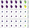 |
Fig. B.1. 2D maps of light and mass fractions of stellar populations binned by age. Each panel is analogous to a bin in a histogram, so this is equivalent to a "spatially resolved histogram". The top galaxy is CAVITY52731, the middle one is CAVITY52732, and the bottom one is CAVITY52733. |
Appendix C: Comparison with MaNGA triplets
In this section we present a brief qualitative comparison between our triplets and two triplets from the SIT catalog (Argudo-Fernández et al. 2015). To the best of our knowledge, there is no sample of IFU observed triplets that could be used as a control sample to make direct comparisons. Among the 315 SIT galaxies, only two systems have all three galaxies observed by MaNGA. Those are SIT 10 and SIT 178 (see Fig. C.1).
Both systems have a late-type central (most massive) galaxy. This is already distinct from our sample, as VSG31 has a late-type central galaxy, but CAVITY5273X have an early-type central galaxy. Additionally, their geometrical configurations are very distinct. Both SIT triplets consist of a pair of close galaxies in projection, with a third, further member. The systems seem less compact than VGS31 and CAVITY5273X.
In conclusion, the number of IFU observed triplets is still very low, making it difficult to get to statistical conclusions and compare specific cases with bigger samples. Further spatially resolved SPS should also be applied to these MaNGA triplets to enhance the quantity and quality of information we have about isolated triplets.
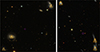 |
Fig. C.1. Three color images, taken from SDSS SkyViewer, of triplets from SIT catalog (Argudo-Fernández et al. 2015): SIT10 (left) and SIT178 (right). |
All Tables
Stellar population characteristics computed through FADO with the integrated spectra.
Emission lines fluxes and ratios, and BPT and WHAN classification computed through FADO with the integrated spectra (fluxes are in units of ×1016 erg/s/cm2).
All Figures
|
Fig. 1. RGB images of the two triplets taken from DESI Legacy Survey. The left panel shows the VGS31 triplet, with VGS31a in the center, VGS31b to its southeast, and VGS31c to its west. The right panel shows CAVITY5273X, with CAVITY52731 to the east, CAVITY52732 to its west, and CAVITY52733 to its southwest. |
| In the text | |
|
Fig. 2. Comparison of the ⟨log t⟩L map for the galaxy CAVITY52731 before (left) and after (right) applying INLA. |
| In the text | |
|
Fig. 3. Maps of luminosities of the galaxies, with the colored lines indicating different contours of S/N. The red contour is for S/N ≥ 10, the green for 5, and the blue for 3. The S/Ns were computed in the wavelength interval of 4000−4060 Å. |
| In the text | |
|
Fig. 4. 2D maps of luminosities, SFR surface densities, mean stellar ages and metallicities, for all six galaxies in our sample. |
| In the text | |
|
Fig. 6. BPT diagram (left) and WHAN diagram (right) for the galaxies in this work, obtained from the integrated spectra. |
| In the text | |
|
Fig. 7. Stellar mass assembly function for the galaxies in triplets. The functions are the mean of the 100 different curves generated with Monte Carlo after perturbing the spectra and applying FADO in each of them. The shaded regions represent the error of the mean. These functions were obtained from the integrated spectra. |
| In the text | |
|
Fig. 5. Maps of BPT classification for the galaxies. Blue is for star-forming spectra, green for composite, yellow for LINER-like emission, and red for Seyfert. |
| In the text | |
|
Fig. 8. Mass-metallicity relation for the galaxies in our sample. In blue we have the MMR for void galaxies, taken from Domínguez-Gómez et al. (2023a). The dashed lines are the mean values, the shaded regions are the error of the mean, and the dotted lines mark the 1σ distribution in metallicity. The MMR is shown for three different samples: all void galaxies (from CAVITY), ST-SFH void galaxies, and LT-SFH void galaxies. The black dots indicate the masses and central metallicities of the galaxies in our sample. The points are the mean of the 100 different points generated for each galaxy with Monte Carlo after perturbing the spectra and applying FADO in each of them. The error bars indicate the standard deviation of the Monte Carlo generated sample. |
| In the text | |
|
Fig. 9. MORFOMETRYKA output for CAVITY 52731 (upper row), CAVITY 52732 (middle), and CAVITY 52733 (lower). In the columns, from left to right: original image in g band (arcsinh scale); single Sérsic model fit and PSF (lower left insert); single Sérsic residual; asymmetry map; and brightness profile (black dots) and 1D (yellow) and 2D (red) derived Sérsic models. In the leftmost panels, the dark green line is the initial segmentation region; the neon green lines are the two Petrosian radius regions (obtained both by fitting Sérsic and by image momenta); the red line corresponds to the Sérsic Rn. In the rightmost panels, black dots and bars are measurements and associated uncertainties; the yellow line is the Sérsic fit to the 1D profile; the red line is the profile but with the parameters obtained from the image (2D) fits. |
| In the text | |
|
Fig. A.1. Map of integrated fluxes of the galaxy VGS31b. The red ellipses represent the isophotes fit with PHOTUTILS. |
| In the text | |
|
Fig. A.2. Mean radial profiles of < log t> L (top left), < log t> M (top right), < Z> L (bottom left), and < Z> M (bottom right). The curves were computed after performing a Monte Carlo, perturbing the mean value in each annulus 1000 times and then computing the mean of the 1000 generated curves. The shaded regions are the error of the mean. |
| In the text | |
|
Fig. B.1. 2D maps of light and mass fractions of stellar populations binned by age. Each panel is analogous to a bin in a histogram, so this is equivalent to a "spatially resolved histogram". The top galaxy is CAVITY52731, the middle one is CAVITY52732, and the bottom one is CAVITY52733. |
| In the text | |
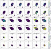 |
Fig. B.2. Same as Fig. B.1 but for (from top to bottom) VGS31a, VSG31b, and VGS31c. |
| In the text | |
|
Fig. C.1. Three color images, taken from SDSS SkyViewer, of triplets from SIT catalog (Argudo-Fernández et al. 2015): SIT10 (left) and SIT178 (right). |
| In the text | |
Current usage metrics show cumulative count of Article Views (full-text article views including HTML views, PDF and ePub downloads, according to the available data) and Abstracts Views on Vision4Press platform.
Data correspond to usage on the plateform after 2015. The current usage metrics is available 48-96 hours after online publication and is updated daily on week days.
Initial download of the metrics may take a while.