| Issue |
A&A
Volume 706, February 2026
|
|
|---|---|---|
| Article Number | A371 | |
| Number of page(s) | 22 | |
| Section | Extragalactic astronomy | |
| DOI | https://doi.org/10.1051/0004-6361/202556328 | |
| Published online | 24 February 2026 | |
Euclid: The first statistical census of dusty and massive objects in the ERO/Perseus field★
1
Dipartimento di Fisica e Astronomia “G. Galilei”, Università di Padova Via Marzolo 8 35131 Padova, Italy
2
INAF-Osservatorio Astronomico di Padova Via dell’Osservatorio 5 35122 Padova, Italy
3
Dipartimento di Fisica e Astronomia “G. Galilei”, Università di Padova Vicolo dell’Osservatorio 3 35122 Padova, Italy
4
Max-Planck-Institut für Astronomie Königstuhl 17 69117 Heidelberg, Germany
5
INAF-Osservatorio di Astrofisica e Scienza dello Spazio di Bologna Via Piero Gobetti 93/3 40129 Bologna, Italy
6
Department of Astronomy, University of Massachusetts Amherst MA 01003, USA
7
School of Physics and Astronomy, Cardiff University, The Parade Cardiff CF24 3AA, UK
8
Institute of Cosmology and Gravitation, University of Portsmouth Portsmouth PO1 3FX, UK
9
Kapteyn Astronomical Institute, University of Groningen PO Box 800 9700 AV Groningen, The Netherlands
10
Cosmic Dawn Center (DAWN)
11
Dipartimento di Fisica e Astronomia, Università di Bologna Via Gobetti 93/2 40129 Bologna, Italy
12
Jeremiah Horrocks Institute, University of Central Lancashire Preston PR1 2HE, UK
13
Université de Strasbourg, CNRS, Observatoire Astronomique de Strasbourg, UMR 7550 67000 Strasbourg, France
14
Université Paris-Saclay, CNRS, Institut d’Astrophysique Spatiale 91405 Orsay, France
15
ESAC/ESA, Camino Bajo del Castillo, s/n Urb. Villafranca del Castillo 28692 Villanueva de la Cañada Madrid, Spain
16
INAF-Osservatorio Astronomico di Brera Via Brera 28 20122 Milano, Italy
17
Université Paris-Saclay, Université Paris Cité, CEA, CNRS, AIM 91191 Gif-sur-Yvette, France
18
IFPU, Institute for Fundamental Physics of the Universe Via Beirut 2 34151 Trieste, Italy
19
INAF-Osservatorio Astronomico di Trieste Via G. B. Tiepolo 11 34143 Trieste, Italy
20
INFN, Sezione di Trieste Via Valerio 2 34127 Trieste TS, Italy
21
SISSA, International School for Advanced Studies Via Bonomea 265 34136 Trieste TS, Italy
22
INFN-Sezione di Bologna Viale Berti Pichat 6/2 40127 Bologna, Italy
23
Dipartimento di Fisica, Università di Genova Via Dodecaneso 33 16146 Genova, Italy
24
INFN-Sezione di Genova Via Dodecaneso 33 16146 Genova, Italy
25
Department of Physics “E. Pancini”, University Federico II Via Cinthia 6 80126 Napoli, Italy
26
INAF-Osservatorio Astronomico di Capodimonte Via Moiariello 16 80131 Napoli, Italy
27
Instituto de Astrofísica e Ciências do Espaço, Universidade do Porto, CAUP Rua das Estrelas PT4150-762 Porto, Portugal
28
Faculdade de Ciências da Universidade do Porto Rua do Campo de Alegre 4150-007 Porto, Portugal
29
Dipartimento di Fisica, Università degli Studi di Torino Via P. Giuria 1 10125 Torino, Italy
30
INFN-Sezione di Torino Via P. Giuria 1 10125 Torino, Italy
31
INAF-Osservatorio Astrofisico di Torino Via Osservatorio 20 10025 Pino Torinese (TO), Italy
32
European Space Agency/ESTEC Keplerlaan 1 2201 AZ Noordwijk, The Netherlands
33
Institute Lorentz, Leiden University Niels Bohrweg 2 2333 CA Leiden, The Netherlands
34
Leiden Observatory, Leiden University Einsteinweg 55 2333 CC Leiden, The Netherlands
35
INAF-IASF Milano Via Alfonso Corti 12 20133 Milano, Italy
36
Centro de Investigaciones Energéticas, Medioambientales y Tecnológicas (CIEMAT) Avenida Complutense 40 28040 Madrid, Spain
37
Port d’Informació Científica, Campus UAB C. Albareda s/n 08193 Bellaterra (Barcelona), Spain
38
Institute for Theoretical Particle Physics and Cosmology (TTK), RWTH Aachen University 52056 Aachen, Germany
39
INAF-Osservatorio Astronomico di Roma Via Frascati 33 00078 Monteporzio Catone, Italy
40
INFN Section of Naples Via Cinthia 6 80126 Napoli, Italy
41
Institute for Astronomy, University of Hawaii 2680 Woodlawn Drive Honolulu HI 96822, USA
42
Dipartimento di Fisica e Astronomia “Augusto Righi” – Alma Mater Studiorum Università di Bologna Viale Berti Pichat 6/2 40127 Bologna, Italy
43
Instituto de Astrofísica de Canarias Vía Láctea 38205 La Laguna Tenerife, Spain
44
Institute for Astronomy, University of Edinburgh, Royal Observatory Blackford Hill Edinburgh EH9 3HJ, UK
45
Jodrell Bank Centre for Astrophysics, Department of Physics and Astronomy, University of Manchester Oxford Road Manchester M13 9PL, UK
46
European Space Agency/ESRIN Largo Galileo Galilei 1 00044 Frascati Roma, Italy
47
Université Claude Bernard Lyon 1, CNRS/IN2P3, IP2I Lyon, UMR 5822 Villeurbanne F-69100, France
48
Institut de Ciències del Cosmos (ICCUB), Universitat de Barcelona (IEEC-UB) Martí i Franquès 1 08028 Barcelona, Spain
49
Institució Catalana de Recerca i Estudis Avançats (ICREA) Passeig de Lluís Companys 23 08010 Barcelona, Spain
50
UCB Lyon 1, CNRS/IN2P3, IUF, IP2I Lyon 4 Rue Enrico Fermi 69622 Villeurbanne, France
51
Mullard Space Science Laboratory, University College London, Holmbury St Mary Dorking Surrey RH5 6NT, UK
52
Departamento de Física, Faculdade de Ciências, Universidade de Lisboa, Edifício C8 Campo Grande PT1749-016 Lisboa, Portugal
53
Instituto de Astrofísica e Ciências do Espaço, Faculdade de Ciências, Universidade de Lisboa, Campo Grande 1749-016 Lisboa, Portugal
54
Department of Astronomy, University of Geneva Ch. d’Ecogia 16 1290 Versoix, Switzerland
55
INAF-Istituto di Astrofisica e Planetologia Spaziali, Via del Fosso del Cavaliere 100 00100 Roma, Italy
56
INFN-Padova Via Marzolo 8 35131 Padova, Italy
57
Aix-Marseille Université, CNRS/IN2P3, CPPM Marseille, France
58
Space Science Data Center, Italian Space Agency Via del Politecnico snc 00133 Roma, Italy
59
School of Physics, HH Wills Physics Laboratory, University of Bristol Tyndall Avenue Bristol BS8 1TL, UK
60
Universitäts-Sternwarte München, Fakultät für Physik, Ludwig-Maximilians-Universität München Scheinerstrasse 1 81679 München, Germany
61
Max Planck Institute for Extraterrestrial Physics Giessenbachstr. 1 85748 Garching, Germany
62
Institute of Theoretical Astrophysics, University of Oslo P.O. Box 1029 Blindern 0315 Oslo, Norway
63
Jet Propulsion Laboratory, California Institute of Technology 4800 Oak Grove Drive Pasadena CA 91109, USA
64
Department of Physics, Lancaster University Lancaster LA1 4YB, UK
65
Felix Hormuth Engineering Goethestr. 17 69181 Leimen, Germany
66
Technical University of Denmark Elektrovej 327 2800 Kgs. Lyngby, Denmark
67
Cosmic Dawn Center (DAWN)
68
Institut d’Astrophysique de Paris, UMR 7095, CNRS, and Sorbonne Université 98 bis Boulevard Arago 75014 Paris, France
69
NASA Goddard Space Flight Center Greenbelt MD 20771, USA
70
Department of Physics and Helsinki Institute of Physics Gustaf Hällströmin katu 2 00014 University of Helsinki, Finland
71
Université de Genève, Département de Physique Théorique and Centre for Astroparticle Physics 24 quai Ernest-Ansermet CH-1211 Genève 4, Switzerland
72
Department of Physics P.O. Box 64 00014 University of Helsinki, Finland
73
Helsinki Institute of Physics, Gustaf Hällströmin katu 2, University of Helsinki Helsinki, Finland
74
Laboratoire d’etude de l’Univers et des phenomenes eXtremes, Observatoire de Paris, Université PSL, Sorbonne Université, CNRS 92190 Meudon, France
75
Aix-Marseille Université, CNRS, CNES, LAM Marseille, France
76
SKA Observatory, Jodrell Bank, Lower Withington, Macclesfield Cheshire SK11 9FT, UK
77
Centre de Calcul de l’IN2P3/CNRS 21 Avenue Pierre de Coubertin 69627 Villeurbanne Cedex, France
78
Dipartimento di Fisica “Aldo Pontremoli”, Università degli Studi di Milano Via Celoria 16 20133 Milano, Italy
79
INFN-Sezione di Milano Via Celoria 16 20133 Milano, Italy
80
University of Applied Sciences and Arts of Northwestern Switzerland, School of Computer Science 5210 Windisch, Switzerland
81
Universität Bonn, Argelander-Institut für Astronomie Auf dem Hügel 71 53121 Bonn, Germany
82
INFN-Sezione di Roma, Piazzale Aldo Moro 2 – c/o Dipartimento di Fisica, Edificio G. Marconi 00185 Roma, Italy
83
Dipartimento di Fisica e Astronomia “Augusto Righi” – Alma Mater Studiorum Università di Bologna Via Piero Gobetti 93/2 40129 Bologna, Italy
84
Department of Physics, Institute for Computational Cosmology, Durham University South Road Durham DH1 3LE, UK
85
Université Côte d’Azur, Observatoire de la Côte d’Azur, CNRS, Laboratoire Lagrange, Bd de l’Observatoire, CS 34229 06304 Nice Cedex 4, France
86
Université Paris Cité, CNRS, Astroparticule et Cosmologie 75013 Paris, France
87
CNRS-UCB International Research Laboratory, Centre Pierre Binétruy, IRL2007, CPB-IN2P3 Berkeley, USA
88
Institut d’Astrophysique de Paris 98bis Boulevard Arago 75014 Paris, France
89
Institute of Physics, Laboratory of Astrophysics, Ecole Polytechnique Fédérale de Lausanne (EPFL), Observatoire de Sauverny 1290 Versoix, Switzerland
90
Aurora Technology for European Space Agency (ESA), Camino bajo del Castillo, s/n Urbanizacion Villafranca del Castillo Villanueva de la Cañada 28692 Madrid, Spain
91
Institut de Física d’Altes Energies (IFAE), The Barcelona Institute of Science and Technology, Campus UAB 08193 Bellaterra (Barcelona), Spain
92
School of Mathematics and Physics, University of Surrey, Guildford Surrey GU2 7XH, UK
93
DARK, Niels Bohr Institute, University of Copenhagen Jagtvej 155 2200 Copenhagen, Denmark
94
Waterloo Centre for Astrophysics, University of Waterloo Waterloo Ontario N2L 3G1, Canada
95
Department of Physics and Astronomy, University of Waterloo Waterloo Ontario N2L 3G1, Canada
96
Perimeter Institute for Theoretical Physics Waterloo Ontario N2L 2Y5, Canada
97
Centre National d’Etudes Spatiales – Centre Spatial de Toulouse 18 Avenue Edouard Belin 31401 Toulouse Cedex 9, France
98
Institute of Space Science, Str. Atomistilor Nr. 409 Măgurele Ilfov 077125, Romania
99
Consejo Superior de Investigaciones Cientificas Calle Serrano 117 28006 Madrid, Spain
100
Universidad de La Laguna, Departamento de Astrofísica 38206 La Laguna Tenerife, Spain
101
Caltech/IPAC 1200 E. California Blvd. Pasadena CA 91125, USA
102
Institut für Theoretische Physik, University of Heidelberg Philosophenweg 16 69120 Heidelberg, Germany
103
Institut de Recherche en Astrophysique et Planétologie (IRAP), Université de Toulouse, CNRS, UPS, CNES 14 Av. Edouard Belin 31400 Toulouse, France
104
Université St Joseph; Faculty of Sciences Beirut, Lebanon
105
Departamento de Física, FCFM, Universidad de Chile, Blanco Encalada 2008 Santiago, Chile
106
Universität Innsbruck, Institut für Astro- und Teilchenphysik Technikerstr. 25/8 6020 Innsbruck, Austria
107
Institut d’Estudis Espacials de Catalunya (IEEC), Edifici RDIT, Campus UPC 08860 Castelldefels Barcelona, Spain
108
Satlantis, University Science Park Sede Bld 48940 Leioa-Bilbao, Spain
109
Institute of Space Sciences (ICE, CSIC), Campus UAB, Carrer de Can Magrans s/n 08193 Barcelona, Spain
110
Instituto de Astrofísica e Ciências do Espaço, Faculdade de Ciências, Universidade de Lisboa Tapada da Ajuda 1349-018 Lisboa, Portugal
111
Universidad Politécnica de Cartagena, Departamento de Electrónica y Tecnología de Computadoras Plaza del Hospital 1 30202 Cartagena, Spain
112
INFN-Bologna Via Irnerio 46 40126 Bologna, Italy
113
Infrared Processing and Analysis Center, California Institute of Technology Pasadena CA 91125, USA
114
INAF, Istituto di Radioastronomia Via Piero Gobetti 101 40129 Bologna, Italy
115
Department of Physics, Oxford University Keble Road Oxford OX1 3RH, UK
116
ICL, Junia, Université Catholique de Lille, LITL 59000 Lille, France
★★ Corresponding author: This email address is being protected from spambots. You need JavaScript enabled to view it.
Received:
9
July
2025
Accepted:
14
November
2025
Abstract
Our comprehension of the history of star formation at z > 3 strongly relies on rest-frame ultraviolet observations. However, this selection systematically misses the dustiest and most massive sources, resulting in an incomplete census at earlier times. Infrared facilities such as Spitzer and the James Webb Space Telescope have shed light on a hidden population lying at z = 3 − 6 characterised by extreme red colours named HIEROs (HST-to-IRAC extremely red objects), identified by the colour criterion HE − ch2 > 2.25. Recently, Euclid Early Release Observations (EROs) have opened the possibility to further study such objects, exploiting the comparison between Euclid and ancillary Spitzer/IRAC observations. The aim of this study was to investigate the effectiveness of this synergy in characterising the population of a small test area of 232 arcmin2. We utilised catalogues in the Perseus field across the VIS and NISP bands, supplemented by data from the four Spitzer channels and several ground-based MegaCam bands (u, g, r, Hα, i, and z) already included in the ERO catalogue. We selected 121 HIEROs by applying the HE − ch2 > 2.25 colour cut, cleaned this sample of globular clusters and brown dwarfs, and then inspected by eye the multi-band cutouts of each source, ending with 42 reliable HIEROs. Photometric redshifts and other physical properties of the final sample were estimated using the spectral-energy-distribution-fitting software Bagpipes. From the zphot and M* values, we computed the galaxy stellar mass function at 3.5 < z < 5.5. When we exclude all galaxies that could host an active galactic nucleus, or whose stellar masses might be overestimated, we still find that the high-mass end of the galaxy stellar mass function is similar to previous estimates, indicating that the true value could be even higher. This investigation highlights the importance of a deeper study of this still mysterious population, in particular to assess its contribution to the cosmic star-formation rate density and its agreement with current galaxy evolution and formation models. These early results demonstrate Euclid’s capabilities to push the boundaries of our understanding of obscured star formation across a wide range of epochs.
Key words: methods: observational / galaxies: evolution / galaxies: high-redshift / galaxies: luminosity function / mass function / galaxies: photometry
This paper is published on behalf of the Euclid Consortium.
© The Authors 2026
 Open Access article, published by EDP Sciences, under the terms of the Creative Commons Attribution License (https://creativecommons.org/licenses/by/4.0), which permits unrestricted use, distribution, and reproduction in any medium, provided the original work is properly cited.
This article is published in open access under the Subscribe to Open model. This email address is being protected from spambots. You need JavaScript enabled to view it. to support open access publication.
1. Introduction
Addressing the process of stellar mass assembly over the age of the Universe is fundamental to our understanding of galaxy formation and evolution since it offers critical insights into the processes driving the evolution of structures in the Universe. This becomes even more crucial at early epochs, at z > 3, where the buildup of massive galaxies remains a subject of active investigation. Resolving this fundamental issue remains a central objective of observational extragalactic astronomy given its importance in validating or challenging the predictions of galaxy formation models (Santini et al. 2009).
One technique for finding ‘normal’ high-redshift star-forming galaxies has been to locate the Lyman break between the rest-frame ultraviolet and optical stellar emission (Steidel & Hamilton 1993; Steidel et al. 1995; Madau et al. 1996; Steidel et al. 1999). These ‘Lyman-break galaxies’ are detected because they are much brighter on the long-wavelength side of the break than on the short-wavelength side (Bouwens et al. 2015; Oesch et al. 2016). However, at z > 3 this selection method systematically misses the dustiest massive objects.
Observations with the Spitzer Space Telescope, the Atacama Large Millimeter/submillimeter Array (ALMA), the James Webb Space Telescope (JWST), and radio telescopes have led to the discovery of a population of dust-obscured massive galaxies missed by the Lyman-break technique (e.g. Wang et al. 2019; Gruppioni et al. 2020; Talia et al. 2021; Enia et al. 2022; Gómez-Guijarro et al. 2023; Nelson et al. 2023; Pérez-González et al. 2023; Gardner et al. 2023; Gentile et al. 2024; Gottumukkala et al. 2024). These galaxies have been called optically dark galaxies or HST-dark galaxies due to the fact that they are missed even in the deepest Hubble Space Telescope (HST) observations. Their spectral energy distributions (SEDs) usually have very red slopes.
The contribution of this population to the star-formation rate density may be as much as 10 times higher than the contribution of the galaxies found by the Lyman-break technique at z ≈ 4, and may be even higher at z = 5 − 7 (Wang et al. 2019; Rodighiero et al. 2023; Wang et al. 2025; Traina et al. 2024). Their high stellar masses (Caputi et al. 2012; Gottumukkala et al. 2024) mean that improved knowledge of this population is important for a better understanding of the evolution of the high-mass end of the galaxy stellar mass function (GSMF) in the early Universe.
Euclid (Laureijs et al. 2011; Euclid Collaboration: Mellier et al. 2025), which was launched by the European Space Agency (ESA) in July 2023 to investigate the evolution of dark matter and energy in the Universe, is also well suited to search for these galaxies. It is equipped with two instruments: the visible instrument (VIS; Euclid Collaboration: Cropper et al. 2025), able to obtain high-resolution optical imaging in the IE band, covering a wavelength range between 550 and 900 nm; and the Near-Infrared Spectrometer and Photometer (NISP), which provides spectrophotometric observations in three near-infrared bands (YE, JE, and HE) at 900−2000 nm (Euclid Collaboration: Schirmer et al. 2022; Euclid Collaboration: Jahnke et al. 2025). The deep Euclid
images of the Perseus cluster obtained during the Early Release Observations (EROs; Euclid Early Release Observations 2024; Cuillandre et al. 2025a), coupled with Spitzer observations of this cluster, allow us to search for these optically dark galaxies. In this study we tested Euclid’s ability to search for such high-redshift dark galaxies, focusing on a particular type, the HST-to-IRAC extremely red objects (HIEROs), as defined by Wang et al. (2016) using the colour criterion HE − ch2 > 2.25 (see Caputi et al. 2012 for an introduction to this method). The goal of this work was to compute the GSMF and evaluate the contribution of these red galaxies to the overall mass function.
The paper is structured as follows. In Sect. 2 we provide a brief overview of the images used in this study. In Sect. 3 we describe the procedure used to build our sample and to estimate the physical properties of the galaxies. We present our results in Sect. 4, including our estimates of the GSMF. In Sect. 5 we discuss the possible effects that may have biased our results. Our conclusions are listed in Sect. 6.
Throughout the paper we assume a Λ cold dark matter cosmology with parameters from Planck Collaboration XXIV (2016) and a Chabrier (2003) initial mass function. All magnitudes presented in this work are reported in the AB magnitude system.
2. Multi-wavelength observations and photometry of the Perseus cluster
The Perseus cluster (centred at RA:  , Dec: 41° 30′54″), also known as Abell 426, is at a distance of 72 Mpc, corresponding to z = 0.0167. It extends over more than 50 Mpc and belongs to the Perseus-Pisces supercluster (Wegner et al. 1993; Aguerri et al. 2020). It has been observed by numerous X-ray telescopes (Lau et al. 2017; Sanders et al. 2020), as well as at other wavelengths.
2.1. Euclid Early Release Observations
In this work we analysed the observations of the cluster that were made during the ERO programme1 (Cuillandre et al. 2025b; Marleau et al. 2025). The IE images have a pixel size of  and the NISP images have a pixel size of
  . In the mosaics made from the images, the full width at half maximum (FWHM) values in the IE, YE, JE, and HE bands are
  ,
,  ,
,  , and
, and  , respectively (Cuillandre et al. 2025b). These FWHM values correspond to 56 pc for VIS and 170 pc for NISP at the distance of the Perseus cluster. We also used in our analysis observations of the cluster that were made with MegaCam at the Canada-France-Hawaii Telescope (CFHT) in the u, g, r, i, z, and Hα ‘off’ filters (Euclid Collaboration: Zalesky et al. 2025).
We used the catalogues of the sources provided by the Euclid Consortium. Not all the sources detected in the HE band were detected in the IE band, given that these catalogues were obtained by running SExtractor (Source Extractor; Bertin & Arnouts 1996) separately on the IE band and a combination of the three NISP images (Cuillandre et al. 2025b). We used the MAG_AUTO measurements, automatically obtained by SExtractor within a Kron-like elliptical aperture, thus minimising the need for additional corrections. In fact, this measurement estimates the total flux by integrating the pixel values within an aperture that is adaptively scaled according to each source’s light distribution, thereby adjusting to its intrinsic morphology. We corrected for Galactic extinction using the formula mintrinsic = mobserved − C E(B − V) with E(B − V) = 0.16 and the values of the parameters given in the README file and in Table 1. The extinction was derived using the dust extinction curve of Gordon et al. (2023) and Gordon (2024).
Values applied to correct for Galactic extinction in the different filters.
2.2. Spitzer imaging and catalogue extraction
The Perseus cluster has been surveyed by the Spitzer Space Telescope (Werner et al. 2004) in various programmes and observing modes, mostly aimed at studying the core of the cluster. We took advantage of the reduced and calibrated products available from the archive. For this work, we downloaded the Infrared Array Camera (IRAC) post-basic calibrated data products, including observations in the four channels (from Programme IDs 3228 and 80089, P.Is. W. Forman and D. Sanders, respectively).
We used the two pointings that are within the area of the cluster imaged by Euclid, which cover a total area of 232 arcmin2. The four IRAC wavelengths are 3.6 μm (ch1), 4.5 μm (ch2), 5.7 μm (ch3), and 8 μm (ch4). For the first pointing there were only useful data in ch1, ch2, and ch3, while for the second pointing there were only useful data in ch1, ch2, and ch4. The layout of the Euclid and Spitzer images are shown in Fig. 1, where the difference in the sizes of the images provided by the two telescopes can be clearly seen.
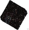 |
Fig. 1. Euclid red-green-blue image of the Perseus cluster made by combining the images taken through the three NISP filters. The solid coloured lines show the extent of the two Spitzer/IRAC datasets, with the cyan and magenta lines showing the extent of the first and second pointings, respectively. The images have been aligned with the WCS coordinate system, with north up and east to the left. In the low-right corner, a scale bar representing 5 arcmin is shown. |
We used the SExtractor set-up described by Moneti et al. (2022) to detect sources in the Spitzer images, with the only change being that we lowered the values of DETECT_THRESH and ANALYSIS_THRESH from 2 to 1 in order to find the faintest objects. The parameters we used are listed in Table 2. To convert the fluxes in the IRAC maps from MJy sr−1 to AB magnitudes, we used the flux density for a zeroth magnitude star of 3631 Jy and a pixel size  2.
2.
Key parameters used for the SExtractor analysis of the Spitzer images.
We used the 4.5 μm images as detection images, using SExtractor in dual mode to derive the fluxes in the other channels. In order for SExtractor to run in this mode, we had to convert the images in the different channels to a common size. For the first pointing, we converted the ch1 and ch3 images to the same size as the ch2 image using the reproject package. For the second pointing, we expanded the size of the ch1 image to match the size of the ch2 image by adding a blank boundary. As result, some of the sources detected in the ch2 image do not have observations in ch1.
Although the Galactic extinction at these wavelengths is very small, we applied the same procedure as we used for the other images (see Sect. 2.1). However, we had to calculate our own corrections, since Spitzer data are not included in the Euclid ERO catalogues. We used the same E(B − V) value as before and calculate the C factors using the dust_extinction Python package (Gordon 2024). The extinction values are listed in Table 1.
We used the MAG_AUTO magnitudes obtained from SExtractor, as in the Euclid case, ensuring consistency among the colours derived in the combined photometric catalogue (see Sect. 3.1). We considered all detections with signal-to-noise ratio (S/N) greater than 3. If a galaxy was detected with a lower S/N, we gave it a magnitude limit corresponding to 3σ.
3. Methods
3.1. A cross-matched Spitzer–Euclid catalogue
We matched the Spitzer catalogue with the Euclid NISP catalogue using TOPCAT (Taylor 2005) with a matching radius of  . The radius chosen may seem small, considering that IRAC positions can substantially move due to the presence of blending. However, most sources presenting a blending problem in the IRAC images would have been discarded anyway during the visual check (see below). Therefore, we adopted this conservative choice to end up only with candidates having reliable photometry. After combining the Euclid NISP and Spitzer catalogues, we used TOPCAT to match the sources to the VIS and MegaCam catalogues, using the same matching radius.
The Spitzer catalogue from the first pointing contains 3294 objects, whereas the matched catalogue contains 1939 objects having both Euclid NISP and Spitzer ch2 detections. Thus, 1355 objects do not have a Euclid counterpart. For the second pointing, the initial Spitzer catalogue has 5793 objects, but only 3377 also have a Euclid NISP detection, so 2416 lack a Euclid counterpart.
In Table 3 we report the magnitude limits (at 1σ) in all bands. For Euclid, we simply scaled the S/N values in the Euclid catalogues to obtain the 1σ values. For Spitzer, we determined the noise by placing 100 circular apertures randomly in background areas of the images, ensuring they did not overlap with sources by checking the segmentation maps provided by SExtractor. We used the Python package photutils (Bradley et al. 2024) to measure the fluxes in these apertures and the mean value of these measurements as our estimate of the noise.
Magnitude limits (1σ) for the data used in this paper.
3.2. HIERO sample selection
To identify the candidate HIEROs in the matched Euclid+Spitzer catalogue, we used the colour criterion of Wang et al. (2016), HE − ch2 > 2.25. This criterion provided us with an initial sample of 121 objects (50 from pointing 1 and 71 from pointing 2). Figure 2 shows the parent sample and the objects found with the colour cut. There were 18 objects detected in the combined NISP image but that were not detected in the HE image; we show them with a triangle symbol (using the 1σHE limit for clarity on the plot).
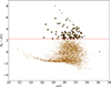 |
Fig. 2. Colour-magnitude (HE − ch2 versus ch2) distribution of the matched Euclid and Spitzer sample. The yellow stars show the objects that satisfy the HIERO colour criterion (shown as a dashed red line). The triangle symbols show lower limits for the HE-undetected objects, calculated using the 1σHE magnitude limit. The other points show the parent sample. |
We performed a visual inspection of the Spitzer/IRAC and Euclid VIS and NISP images to spot objects that might be artefacts or noise features. We removed 69 objects, reducing our sample to 52. Figure 3 provides an example of the discarded objects. To retain only reliable objects, we proceeded with a further series of tests (see Sects. 3.3, 3.4, and 3.5).
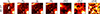 |
Fig. 3. Example multi-wavelength cutout of an object that was discarded due to an artefact in the VIS image. The cutout sizes are 15″ × 15″. |
3.3. Blending contamination in the IRAC photometry
Through the visual check on the Euclid VIS and NISP+Spitzer cutouts (see Fig. A.1), we identified a few objects that appeared to have several components in the VIS and NISP bands. We checked that the extraction executed in all the available bands treated these multi-component objects as a single source. This means that in all the bands the different components have been detected as a single source, therefore not invalidating the photometry by being a single source in some bands and two different sources in others (for a more detailed discussion of these objects, see Sect. 5.2).
3.4. Globular cluster contamination
We removed possible globular clusters (GCs) by applying the selection criteria used for the Fornax cluster ERO data (Saifollahi et al. 2025). The GCs in Fornax were selected as: (1) being partially resolved and with small eccentricity; and (2) having colours 0.0 < IE − YE < 0.8, −0.3 < YE − JE < 0.5, and −0.3 < JE − HE < 0.5. To be conservative, we decided to consider as GCs all objects that satisfied the colour conditions, independent of their size. Ultimately, nine candidates satisfied these conditions, reducing our sample to 43 objects.
3.5. Brown dwarf contamination
We fitted the SEDs of the 43 remaining objects with brown dwarf templates from Burrows et al. (2006). We used the T dwarf models, which cover a temperature range from 700 K to 2200 K, gravities between 104.5 and 105.5 cm s−2, and metallicities between [Fe/H] = −0.5 and 0.5. We then compared the χ2 of the fit with the χ2 of the fit with the galaxy templates (see the next section), removing any object with a better fit to a brown dwarf template. There was only one of these (ID 39), giving us a final sample of 42 objects.
3.6. SED fitting analyses
We fitted the SEDs of the 42 remaining objects with the Bagpipes package (Carnall et al. 2018). For all the candidates with no photometric detection in a specific band, we set the flux to 0 and the error to 3σ (see Sect. 3). We adopted a Bagpipes set-up that maximises the exploration of the parameter space. We used a Calzetti law (Calzetti et al. 2000) for the dust extinction, a ‘delayed’ star-formation history, and we included the nebular emission component, to allow for the effect of emission lines on the SED, which might otherwise lead to an overestimate of the stellar masses (Sect. 5.1.1). The broad range used for the dust extinction value is essential for this particular type of galaxy, since they are expected to be very dusty. Table 4 lists the parameters adopted as the input set up for the fitting code.
Main input parameters for Bagpipes.
After the first run of Bagpipes, we noticed that for two objects in the final sample, IDs 23 and 31, the MegaCam fluxes were suspiciously high with respect to the others, in particular relative to the flux in the IE band. For object 23, the fluxes in the two MegaCam filters on either side of the IE band, the Hα and i bands, were, respectively, a factor of 1.3 and 2.5 higher than the IE flux. For object 31, the fluxes in the Hα and i filters were 30 and 15 times higher, respectively, than the IE flux. To investigate the reasons behind these examples, we visually checked the Euclid VIS and NISP + Spitzer cutouts of these objects. We concluded that the fluxes measured from the MegaCam images, which have lower resolution than the Euclid images, are likely to be contaminated by nearby objects visible in the Euclid images. For these two objects, we performed a second run of Bagpipes, excluding the MegaCam data. We use the results of these fits in the rest of the paper.
4. Results
Before presenting the outcome of our work, we want to stress that we relied on only a few photometric data points. Even if upper limits are taken into account in the SED fitting analyses, sometimes we have just three or four detections with S/N > 3. For this reason, we invite the reader to be cautious about the photometric redshifts retrieved and the galaxies properties estimated.
4.1. Main SED-fitting categories
Figure 4 shows an example of the main categories of fits. All the fits are shown in Fig. A.2. We show three different fits: fits with the lowest χ2, the fit chosen by Bagpipes, which is the fit for the median value of the posterior probability distribution, and the best fit for the redshift value with the highest probability, the peak in the redshift probability distribution function (PDF(z)). If some of the fits are not visible, it means that they are hidden by the others. We decided to use this final fit in the rest of the paper because this avoids any problems caused by the effect on the physical parameters if there is a bimodal PDF(z). For this reason, in the rest of this paper we use the peak in the PDF(z) as the photometric redshift of the object and the physical properties estimated with this redshift, in particular the dust attenuation AV and the stellar mass M* values.
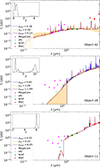 |
Fig. 4. Bagpipes fits to the SEDs for three representative objects, IDs 42, 28, and 11. The posterior PDF(z) are shown as insets. Photometric detections are shown by the coloured circles, and 3σ upper limits are plotted as triangles. The coloured lines show the three different fits described in the text. The PDF for ID 42 peaks at a low redshift, ID 28 is bimodal, and ID 11 has a single high-redshift peak, making it representative of the objects likely to be HIEROs. |
There are three categories of fit shown in Fig. 4: a low-z solution; a bimodal PDF(z); and a typical HIERO candidate. The Bagpipes fit of ID 42 suggests that the object is actually at low redshift. The fit for ID 28, on the other hand, shows a bimodal PDF(z), with a low-z solution and a very high-z (z > 7) one. As previously mentioned, we always selected the solution corresponding to the peak of the probability distribution function (PDF), in this case the low-z solution. Finally, object ID 11 is an example of a typical HIERO source. The PDF(z) shows a clear peak at z ≈ 6, with all three fits in agreement that the object is at high redshift. We also find HIEROs at lower redshifts (z = 3 − 4); all the fits are shown in Appendix A.
4.2. Physical properties
The physical properties derived from the Bagpipes fits are given in Table A.1 for all 42 objects in the sample. We show in Fig. 5 the main physical properties as a function of redshift, in particular the dust extinction and stellar mass. We do not discuss the star formation rate estimates here since they are not reliable, given the lack of far-infrared data. The outlier point in the plots is for ID 13, which has an estimated redshift of 14.6, although this result is uncertain due to the multi-peak behaviour of the redshift probability distribution (for further discussion regarding this source see Sect. 5.3).
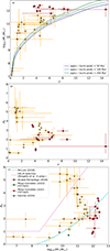 |
Fig. 5. Properties of the HIEROs. Panel (a): Redshift versus stellar mass. The red circles show the most massive candidates, with stellar mass greater than 1011.7 M⊙. These objects are from here on defined as ‘over-massive’ and shown with the same symbol, i.e. red circles, in all other panels. The solid lines report the minimum observable stellar mass producing an IRAC ch2 magnitude of 22.7. All three curves represent star-forming galaxies, the green with an age between the redshift epoch and the burst peak of 200 Myr, the teal one 100 Myr, and the dark blue one 50 Myr. Panel (b): Redshift versus dust attenuation distribution. Panel (c): Dust attenuation versus stellar mass. The solid cyan line shows the relation from McLure et al. (2018), while the magenta line delimits the area identifying the so-called HELM galaxies (Bisigello et al. 2025). Different symbols report values from previous studies, as indicated in the legend. |
The mean photometric redshift of the sample is approximately 4. The top right panel of Fig. 5 shows that the majority of the objects have high values of dust extinction, with a mean value of AV = 2.8, confirming that this kind of object is indeed dusty (to obtain these high values, it was necessary to allow the dust extinction parameter to cover a wide range of values, up to AV = 6). The trend is similar to the one found by Bisigello et al. (2023) for fainter galaxies observed with JWST. The second and third panels of Fig. 5 show that the galaxies generally have more extinction than the relationship between extinction and stellar mass found for normal galaxies by McLure et al. (2018). We also show the relationship for highly extincted low-mass (HELM) galaxies (Bisigello et al. 2025). Seven of the galaxies in our sample have extinction values that are above this relationship, while 16 galaxies have extinction values between the two relationships.
We can see that, as expected, stellar mass increases with redshift. The mean value of log10(M*/M⊙) = 10.9 clearly shows that we indeed find very massive galaxies. We highlight the most massive galaxies, defined as log10(M*/M⊙) > 11.7, in Fig. 5. We discuss these galaxies in Sect. 4.3.
4.3. Stellar mass functions of HIEROs at z = 3.5 − 5.5
The GSMFs in the Perseus field have been derived by adopting the best-fit photometric redshifts and stellar mass estimates given in Table A.1. GSMFs have been calculated in a single redshift bin, spanning from 3.5 to 5.5, to achieve better statistics given the low number of data points. We intentionally decided to focus the analysis on this redshift range to investigate the contributions of the HIERO population to the stellar mass assembly beyond cosmic noon.
The GSMFs have been derived following the technique described in Fontana et al. (2006), Santini et al. (2012), and Grazian et al. (2015). In detail, for each galaxy with 3.5 ≤ zphot ≤ 5.5 and magnitude in ch2 above the completeness limit (i.e. [ch2] = 20.9 AB), we derived the non-parametric GSMF as the sum of the inverse accessible volumes.
The GSMFs have been limited to a stellar mass above 1.6 × 10¹¹ M⊙ at 3.5 < z < 5.5, corresponding to the magnitude limit in ch2 of the Perseus field, as described in Sect. 3.1. The error bars for each point have been computed using the approach of Gehrels (1986), which is Poisson statistics with proper corrections for small number counts below ten objects. In order to take into account the uncertainties on the photometric redshift derivation or on the stellar mass estimate, we generated 104 synthetic catalogues by randomly sampling every time for each observed object the PDF(z) and its associated stellar mass PDF produced by Bagpipes. We derived the GSMF for each synthetic catalogue, and then we computed the uncertainties of the 104 random GSMFs for each bin in redshift and stellar mass. This error was summed in quadrature with the statistical error of the observed GSMFs, as described above.
We also included the sampling variance in our error estimates in order to take the finite volume sampled into account and to avoid underestimating the total error budget. This variance has been derived by adopting the Cosmic Variance Calculator3 by Trenti & Stiavelli (2008). We assumed an area of 232 arcmin2, a mean redshift of 4.5, with a redshift interval of 2.0, i.e. the one adopted here for the GSMF calculation. The other free parameters in the computation are the number of objects (42), the halo filling factor4 (1.0) and the completeness of the observations (1.0). We assumed both a halo filling factor and a completeness fraction of 1.0 in order to maximise the amount of sample variance. For lower values of the halo filling factor and/or of the completeness fraction, the calculated variance would be lower. The resulting relative sampling variance is 0.17 dex, which has been summed in quadrature with the GSMF errors listed above.
We considered the results from Forrest et al. (2024), who point out that SED fitting tools are not able to properly reproduce the spectrum of red sources similar to those studied in this work. They concluded that stellar mass values exceeding log10(M*/M⊙) > 11.7 in the redshift range 3 < z < 4, derived through SED fitting, are unreliable due to incorrect zphot estimates. Briefly, they selected a sample of galaxies with photometric redshifts between 3 and 4 and stellar mass values above 1011.7 M⊙, which they followed up spectroscopically. They found that the spectroscopic redshifts did not agree with the photometric ones (Δz > 0.5), generally lying below zspec = 2.5.
Taking account of these results, we created a subsample of galaxies with the same stellar mass and redshift cuts, namely log10(M*/M⊙) > 11.7 and z > 3.5. There were 13 objects in this sample, with six of them showing a secondary peak at z < 3.5 in the Bagpipes redshift distribution. These sources will be referred to as ‘over-massive’ from now on. In the next section we discuss possible effects that could produce errors in the GSMFs, such as the presence of active galactic nuclei (AGNs).
We computed the GSMFs in three different ways: (1) using the whole HIERO sample, including the over-massive sources; (2) removing the AGN candidates (see Sect. 5.1.2), but keeping the over-massive sources; and (3) removing both the AGN candidates and the over-massive sources. The different results are shown in Fig. 6. The figure shows that our estimates of the GSMF in the two highest mass bins are entirely due to the presence of the over-massive galaxies, which therefore vanish when these objects are excluded (i.e. the most conservative case, represented by the filled orange star). Our estimate of the GSMF in the lowest mass bin does not change very much when the AGN and over-massive galaxies are removed. However, our estimate of the GSMF in the second lowest mass bin changes significantly when the AGN and over-massive galaxies are removed.
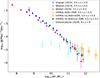 |
Fig. 6. Different GSMFs: with the complete original sample (orange pentagons), with AGN candidates removed (empty orange stars), and with both the AGN candidates and over-massive objects removed, the most conservative case (filled orange stars). The comparison is shown with respect to the values found by Grazian et al. (2015, blue circles) and reported in Weaver et al. (2023, green triangles) and Weibel et al. (2024, magenta squares). The cyan crosses report the values found by Gottumukkala et al. (2024), who applied a similar selection to the JWST/CEERS dataset. |
Nevertheless, even in the most conservative case, when all the AGN and over-massive galaxies are removed, our data points are very similar to previous estimates of the high-mass end of the GSMF. Our estimates are likely to be lower limits because of our very conservative removal of all objects that might possibly be spurious, which suggests that previous estimates of the high-mass end of the GSMF may well be too low. Future Euclid imaging will be crucial for investigating this question further.
5. Discussion
5.1. Overestimates of stellar mass?
In this section we explore effects that might lead to overestimates of the stellar masses and thus produce the over-massive galaxies found in the Bagpipes analysis.
5.1.1. Contribution from line emission
Papovich et al. (2023) pointed out that for a galaxy at z > 4 the absence of a JWST Mid-Infrared Instrument (MIRI) detection at 5.6 and 7.7 μm can lead to an estimate of the stellar mass that is too high by up to a factor of 10. Bisigello et al. (2019) found the same problem for a mock sample of galaxies with data in the JWST NIRCam bands. The error is caused by the contribution of emission lines in broad-band filters, which produce very red colours.
In order to test how much our sample is affected by this issue, we selected only the sources with a clear detection (S/N > 3) in the longer wavelengths bands available, which are IRAC ch3 or ch4, depending on the pointing (as explained in Sect. 2.2). We also required the galaxies to also have detections in the other shorter wavelength IRAC bands, i.e. ch1 and ch2. Only 12 sources are detected in all three IRAC bands. We repeated the SED fitting run reported in Sect. 3.6, this time excluding the measurements for the filter at the longest wavelength. The result was unexpected, with the opposite trend to that described in the aforementioned papers: we found that by removing the last data point, the stellar masses estimated are significantly lower than the case where all the data are considered in the fit. We found seven objects with a difference greater than 1 dex, but in only one case was the stellar mass estimate higher. For the other six, the new stellar mass estimate was lower. The explanation for five of them was that the redshift estimate in the new run was lower, which led to a lower stellar mass estimate. For the remaining galaxy, the two redshift estimates were similar but the new stellar mass estimate was still lower.
To further investigate this result, we performed a second run in which we still excluded the photometry at the longest wavelength, but forced the redshift to be the same as in the original run. We found that for four objects the new stellar mass was still about 1 dex below the original estimate, but for the rest the difference was only about 0.13 dex.
Therefore, we conclude that our stellar masses are not strongly overestimated because of bright nebular emission lines. The difference in the result with respect to the previously mentioned papers might be due to the different sample luminosities. In addition to that, since we used the Bagpipes configuration that allows the nebular parameter to cover a range from −4 to −1 (see Table 4), our results may be less affected by their presence.
5.1.2. AGN contribution
An additional source of uncertainty for the physical properties is the elusive presence of AGNs. If an AGN is present and we are wrongly attributing its emission to stars, we will over-estimate the stellar mass of the galaxy.
To investigate this possibility, we adopted the criteria used inside the Euclid consortium to classify an object as an AGN. The criteria were developed by Bisigello et al. (2021) from the SPRITZ simulation. These criteria distinguish between AGNs1, which are unobscured AGNs, and All-AGNs, which includes obscured AGNs, unobscured AGNs, and galaxies dominated by star-formation with a minor contributions by the AGN.
For the AGN1 classification, the colour selection is IE − HE < 1.1 ∧ u − z < 1.2 ∧ IE − HE < −1.3 (u − z)+1.9, while for the All-AGN classification the colour selection is IE − YE < −0.9 (u − r)+0.8 ∧ u − r < 0.2 (Euclid Collaboration: Bisigello et al. 2024). Only one object satisfies the criteria for both categories (ID 10), while nine fall in the All-AGN class (IDs 1, 2, 4, 22, 26, 29, 36, 37, and 40). However, this colour selection method is tuned with empirical constraints only up to z ≈ 2, and therefore it is not reliable in our case because the majority of our sample is at z > 2. For this reason, we decided to compute the calculation of the GSMFs both including and excluding the AGN candidates.
5.2. Visual morphology
Most of the objects have a compact shape in the VIS image. However, it is worth noting that a few objects have extended structure in the VIS image (the cutouts are shown in Fig. A.1). This could be explained by the presence of a single source composed of multiple components or with an irregular clumpy structure. Another interesting explanation would be the merger between dusty objects, such as the ‘Cosmic Whale’ identified by Rodighiero et al. (2024). This aspect will be explored more in future works.
5.3. A candidate at z ∼ 14
As previously mentioned, with our SED fitting analyses we found a candidate galaxy that appears to be at z ≃ 14 (ID 13). Its multi-wavelength cutout is shown in Fig. 7. In Fig. 8 we show the different Bagpipes fits as explained above, along with the PDF(z). Both the fit with the lowest χ2 and the one corresponding to the highest peak in the PDF(z) give a photometric redshift of around 14.6, whereas the one from the median of the posterior probability distribution predicts the redshift corresponding to the minor peak in the PDF(z) at z = 6.7.
 |
Fig. 7. Multi-wavelength cutouts of ID 13 with an estimated z ≈ 14. The available images are the Euclid bands IE, YE, JE, and HE and the Spitzer channels ch1, ch2, and ch3. The cutout size is 15″ × 15″. |
Input models and main parameters for the CIGALE code.
The stellar mass value found is log10(M*/M⊙) = 12.1, along with a dust extinction of about AV = 1.24 mag (Table A.1). The stellar mass value puts this source among the over-massive objects, while not having a particularly high value for dust extinction, which makes us suspicious of this result. However, we also fit the SED with CIGALE (Boquien et al. 2019), which includes an AGN component in the fit (although we note that this galaxy does not satisfy the Euclid AGN criteria). The parameters used in this fit are listed in Table 5. The fit is shown in the second panel of Fig. 8. The best redshift estimate is also about 14, strengthening the possibility that this galaxy is genuinely at a very high redshift, although the estimate of the stellar mass is now even higher, 1.23 × 10¹³ M⊙. The PDF(z) produced by CIGALE also presents a peak at lower redshift (z < 1).
 |
Fig. 8. SED fits for ID 13: different SED fitting models found by Bagpipes (left) and the fit found by CIGALE (right). Both panels show photometric data points, both detections (circles) and upper limits (triangles). The PDF(z) are displayed in the insets. |
As mentioned before, the few photometric detections available are not enough to robustly constrain the photometric redshift of this source. In addition to this, the probability of finding an object at this redshift in an area of about 232 arcmin2 is less than 10−4, based on the current estimates of the luminosity function (Finkelstein et al. 2024). Hence, this object is likely to be at a lower z than the estimate found through the SED fitting procedures. We think that this object remains of great interest, but spectroscopic observations will be necessary to distinguish between the different possibilities and to determine the true z value.
6. Conclusions
In this work we used Spitzer and Euclid observations (Cuillandre et al. 2025b) of the Perseus cluster to search for HIEROs, dusty galaxies in the redshift range 3 < z < 6. The Spitzer selection allowed us to be certain about the non-spurious nature of these detections, thus avoiding any problem with artefacts in the Euclid images.
In the selection of our final sample we were conservative, both applying a visual check and removing the possible contaminants to assure the robustness of the candidates. Therefore, the number of objects identified should be considered a lower limit. We performed a similar study using the 63 deg2 area from the first Quick Data Release (Q1; Euclid Quick Release Q1 2025), identifying an initial sample of approximately 30 000 HIEROs candidates, which was reduced to 3870 after visual inspection and data cleaning (Euclid Collaboration: Girardi et al. 2025). The surveyed area is smaller in the present work but the observations are deeper, allowing for more robust results. In particular, we were able to examine the SED fittings individually, which was not feasible in the Q1 study due to the sample size. This allowed us to identify distinct categories among the HIERO candidates. Thanks to the improved data quality, we were also able to compute the GSMF for the final sample of 42 objects, which was not possible in the Q1 analysis. The GSMF was calculated in a redshift range between 3.5 and 5.5 and is shown in Fig. 6. The presence of objects with excessive stellar masses is discussed in Sect. 5, where we evaluate different possible explanations. The findings in the work by Forrest et al. (2024) led us to consider different scenarios, where we keep or remove possible biases. Even under the most conservative assumptions, our results remain consistent with the interpretation that we are probing the massive end of the GSMF. This may indicate that previous GSMF estimates were somewhat underestimated, particularly if such objects were not included in the analyses.
Further improvements are expected with the upcoming first data release, which will cover the already observed Euclid Deep Fields at a significantly greater depth, allowing for tighter constraints in the SED fitting. The rarity of these objects makes it difficult to study them with JWST, whose largest contiguous programme covers only 0.6 deg2 (Casey et al. 2024). Their observation requires wide fields of view, which is possible only with the synergy between Euclid and Spitzer.
This case study clearly points to the necessity of delving deeper in the analyses of these sources to be able to correctly characterise them. Above all, the possible unreliability of the retrieved photometric redshift estimates calls attention to the importance of follow-up observations, especially in regards to obtaining spectroscopic data.
Acknowledgments
This work has made use of the Early Release Observations (ERO) data from the Euclid mission of the European Space Agency (ESA), 2024, https://doi.org/10.57780/esa-qmocze3. The Euclid Consortium acknowledges the European Space Agency and a number of agencies and institutes that have supported the development of Euclid, in particular the Agenzia Spaziale Italiana, the Austrian Forschungsförderungsgesellschaft funded through BMK, the Belgian Science Policy, the Canadian Euclid Consortium, the Deutsches Zentrum für Luft- und Raumfahrt, the DTU Space and the Niels Bohr Institute in Denmark, the French Centre National d’Etudes Spatiales, the Fundação para a Ciência e a Tecnologia, the Hungarian Academy of Sciences, the Ministerio de Ciencia, Innovación y Universidades, the National Aeronautics and Space Administration, the National Astronomical Observatory of Japan, the Netherlandse Onderzoekschool Voor Astronomie, the Norwegian Space Agency, the Research Council of Finland, the Romanian Space Agency, the State Secretariat for Education, Research, and Innovation (SERI) at the Swiss Space Office (SSO), and the United Kingdom Space Agency. A complete and detailed list is available on the Euclid web site (www.euclid-ec.org). The Cosmic Variance Calculator was written by M. Trenti & M. Stiavelli with support from NASA JWST grant NAG5-12458. The research activities described in this paper were carried out with contribution of the Next Generation EU funds within the National Recovery and Resilience Plan (PNRR), Mission 4 – Education and Research, Component 2 – From Research to Business (M4C2), Investment Line 3.1 – Strengthening and creation of Research Infrastructures, Project IR0000034 – “STILES – Strengthening the Italian Leadership in ELT and SKA”. The results obtained in this paper are based on observations obtained with MegaPrime/MegaCam, a joint project of CFHT and CEA/DAPNIA, at the Canada-France-Hawaii Telescope (CFHT) which is operated by the National Research Council (NRC) of Canada, the Institut National des Science de l’Univers of the Centre National de la Recherche Scientifique (CNRS) of France, and the University of Hawaii. The observations at the Canada-France-Hawaii Telescope were performed with care and respect from the summit of Maunakea which is a significant cultural and historic site.
References
- Aguerri, J., Girardi, M., Agulli, I., et al. 2020, MNRAS, 494, 1681 [NASA ADS] [CrossRef] [Google Scholar]
- Bertin, E., & Arnouts, S. 1996, A&AS, 117, 393 [NASA ADS] [CrossRef] [EDP Sciences] [Google Scholar]
- Bisigello, L., Caputi, K., Colina, L., et al. 2019, ApJS, 243, 27 [CrossRef] [Google Scholar]
- Bisigello, L., Gruppioni, C., Feltre, A., et al. 2021, A&A, 651, A52 [NASA ADS] [CrossRef] [EDP Sciences] [Google Scholar]
- Bisigello, L., Gandolfi, G., Grazian, A., et al. 2023, A&A, 676, A76 [NASA ADS] [CrossRef] [EDP Sciences] [Google Scholar]
- Bisigello, L., Gandolfi, G., Feltre, A., et al. 2025, A&A, 693, L18 [NASA ADS] [CrossRef] [EDP Sciences] [Google Scholar]
- Boquien, M., Burgarella, D., Roehlly, Y., et al. 2019, A&A, 622, A103 [NASA ADS] [CrossRef] [EDP Sciences] [Google Scholar]
- Bouwens, R. J., Illingworth, G., Oesch, P., et al. 2015, ApJ, 803, 34 [CrossRef] [Google Scholar]
- Bradley, L., Sipőcz, B., Robitaille, T., et al. 2024, https://doi.org/10.5281/zenodo.10967176 [Google Scholar]
- Bruzual, G., & Charlot, S. 2003, MNRAS, 344, 1000 [NASA ADS] [CrossRef] [Google Scholar]
- Burrows, A., Sudarsky, D., & Hubeny, I. 2006, ApJ, 640, 1063 [Google Scholar]
- Calzetti, D., Armus, L., Bohlin, R. C., et al. 2000, ApJ, 533, 682 [NASA ADS] [CrossRef] [Google Scholar]
- Caputi, K. I., Dunlop, J. S., McLure, R. J., et al. 2012, ApJ, 750, L20 [NASA ADS] [CrossRef] [Google Scholar]
- Carnall, A., McLure, R., Dunlop, J., & Davé, R. 2018, MNRAS, 480, 4379 [NASA ADS] [CrossRef] [Google Scholar]
- Casey, C. M., Akins, H. B., Shuntov, M., et al. 2024, ApJ, 965, 98 [NASA ADS] [CrossRef] [Google Scholar]
- Chabrier, G. 2003, PASP, 115, 763 [Google Scholar]
- Cuillandre, J.-C., Bertin, E., Bolzonella, M., et al. 2025a, A&A, 697, A6 [Google Scholar]
- Cuillandre, J.-C., Bolzonella, M., Boselli, A., et al. 2025b, A&A, 697, A11 [Google Scholar]
- Enia, A., Talia, M., Pozzi, F., et al. 2022, ApJ, 927, 204 [NASA ADS] [CrossRef] [Google Scholar]
- Euclid Collaboration (Schirmer, M., et al.) 2022, A&A, 662, A92 [NASA ADS] [CrossRef] [EDP Sciences] [Google Scholar]
- Euclid Collaboration (Bisigello, L., et al.) 2024, A&A, 691, A1 [NASA ADS] [CrossRef] [EDP Sciences] [Google Scholar]
- Euclid Collaboration (Cropper, M., et al.) 2025, A&A, 697, A2 [Google Scholar]
- Euclid Collaboration (Girardi, G., et al.) 2025, A&A, in press, https://doi.org/10.1051/0004-6361/202554615 (Euclid Q1 SI) [Google Scholar]
- Euclid Collaboration (Jahnke, K., et al.) 2025, A&A, 697, A3 [Google Scholar]
- Euclid Collaboration (Mellier, Y., et al.) 2025, A&A, 697, A1 [Google Scholar]
- Euclid Collaboration (Zalesky, L., et al.) 2025, A&A, 695, A229 [Google Scholar]
- Euclid Early Release Observations 2024, https://doi.org/10.57780/esa-qmocze3 [Google Scholar]
- Euclid Quick Release Q1 2025, https://doi.org/10.57780/esa-2853f3b [Google Scholar]
- Finkelstein, S. L., Leung, G. C. K., Bagley, M. B., et al. 2024, ApJ, 969, L2 [NASA ADS] [CrossRef] [Google Scholar]
- Fontana, A., Salimbeni, S., Grazian, A., et al. 2006, A&A, 459, 745 [CrossRef] [EDP Sciences] [Google Scholar]
- Forrest, B., Cooper, M. C., Muzzin, A., et al. 2024, ApJ, 977, 51 [Google Scholar]
- Fritz, J., Franceschini, A., & Hatziminaoglou, E. 2006, MNRAS, 366, 767 [Google Scholar]
- Gardner, J. P., Mather, J. C., Abbott, R., et al. 2023, PASP, 135, 068001 [NASA ADS] [CrossRef] [Google Scholar]
- Gehrels, N. 1986, ApJ, 303, 336 [Google Scholar]
- Gentile, F., Talia, M., Behiri, M., et al. 2024, ApJ, 962, 26 [NASA ADS] [CrossRef] [Google Scholar]
- Gómez-Guijarro, C., Magnelli, B., Elbaz, D., et al. 2023, A&A, 677, A34 [NASA ADS] [CrossRef] [EDP Sciences] [Google Scholar]
- Gordon, K. 2024, J. Open Source Softw., 9, 7023 [NASA ADS] [CrossRef] [Google Scholar]
- Gordon, K. D., Clayton, G. C., Decleir, M., et al. 2023, ApJ, 950, 86 [CrossRef] [Google Scholar]
- Gottumukkala, R., Barrufet, L., Oesch, P., et al. 2024, MNRAS, 530, 966 [NASA ADS] [CrossRef] [Google Scholar]
- Grazian, A., Fontana, A., Santini, P., et al. 2015, A&A, 575, A96 [NASA ADS] [CrossRef] [EDP Sciences] [Google Scholar]
- Gruppioni, C., Béthermin, M., Loiacono, F., et al. 2020, A&A, 643, A8 [NASA ADS] [CrossRef] [EDP Sciences] [Google Scholar]
- Lau, E. T., Gaspari, M., Nagai, D., & Coppi, P. 2017, ApJ, 849, 54 [NASA ADS] [CrossRef] [Google Scholar]
- Laureijs, R., Amiaux, J., Arduini, S., et al. 2011, ArXiv e-prints [arXiv:1110.3193] [Google Scholar]
- Madau, P., Ferguson, H. C., Dickinson, M. E., et al. 1996, MNRAS, 283, 1388 [Google Scholar]
- Marleau, F., Cuillandre, J.-C., Cantiello, M., et al. 2025, A&A, 697, A12 [NASA ADS] [CrossRef] [EDP Sciences] [Google Scholar]
- McLure, R., Dunlop, J., Cullen, F., et al. 2018, MNRAS, 476, 3991 [NASA ADS] [CrossRef] [Google Scholar]
- Meiksin, A. 2006, MNRAS, 365, 807 [Google Scholar]
- Moneti, A., McCracken, H., Shuntov, M., et al. 2022, A&A, 658, A126 [NASA ADS] [CrossRef] [EDP Sciences] [Google Scholar]
- Nelson, E. J., Suess, K. A., Bezanson, R., et al. 2023, ApJ, 948, L18 [NASA ADS] [CrossRef] [Google Scholar]
- Oesch, P., Brammer, G., Van Dokkum, P., et al. 2016, ApJ, 819, 129 [NASA ADS] [CrossRef] [Google Scholar]
- Papovich, C., Cole, J. W., Yang, G., et al. 2023, ApJ, 949, L18 [NASA ADS] [CrossRef] [Google Scholar]
- Pérez-González, P. G., Barro, G., Annunziatella, M., et al. 2023, ApJ, 946, L16 [CrossRef] [Google Scholar]
- Planck Collaboration XXIV. 2016, A&A, 594, A24 [NASA ADS] [CrossRef] [EDP Sciences] [Google Scholar]
- Rodighiero, G., Bisigello, L., Iani, E., et al. 2023, MNRAS, 518, L19 [Google Scholar]
- Rodighiero, G., Enia, A., Bisigello, L., et al. 2024, A&A, 691, A69 [NASA ADS] [CrossRef] [EDP Sciences] [Google Scholar]
- Saifollahi, T., Lançon, A., Cantiello, M., et al. 2025, A&A, 703, A18 [NASA ADS] [CrossRef] [EDP Sciences] [Google Scholar]
- Sanders, J., Dennerl, K., Russell, H., et al. 2020, A&A, 633, A42 [NASA ADS] [CrossRef] [EDP Sciences] [Google Scholar]
- Santini, P., Fontana, A., Grazian, A., et al. 2009, A&A, 504, 751 [NASA ADS] [CrossRef] [EDP Sciences] [Google Scholar]
- Santini, P., Fontana, A., Grazian, A., et al. 2012, A&A, 538, A33 [NASA ADS] [CrossRef] [EDP Sciences] [Google Scholar]
- Schartmann, M., Meisenheimer, K., Camenzind, M., Wolf, S., & Henning, T. 2005, A&A, 437, 861 [NASA ADS] [CrossRef] [EDP Sciences] [Google Scholar]
- Steidel, C. C., & Hamilton, D. 1993, AJ, 105, 2017 [Google Scholar]
- Steidel, C. C., Pettini, M., & Hamilton, D. 1995, AJ, 110, 2519 [Google Scholar]
- Steidel, C. C., Adelberger, K. L., Giavalisco, M., Dickinson, M., & Pettini, M. 1999, ApJ, 519, 1 [NASA ADS] [CrossRef] [Google Scholar]
- Talia, M., Cimatti, A., Giulietti, M., et al. 2021, ApJ, 909, 23 [NASA ADS] [CrossRef] [Google Scholar]
- Taylor, M. B. 2005, ASP Conf. Ser., 347, 29 [Google Scholar]
- Traina, A., Gruppioni, C., Delvecchio, I., et al. 2024, A&A, 681, A118 [NASA ADS] [CrossRef] [EDP Sciences] [Google Scholar]
- Trenti, M., & Stiavelli, M. 2008, ApJ, 676, 767 [Google Scholar]
- Wang, T., Elbaz, D., Schreiber, C., et al. 2016, ApJ, 816, 84 [Google Scholar]
- Wang, T., Schreiber, C., Elbaz, D., et al. 2019, Nature, 572, 211 [Google Scholar]
- Wang, T., Sun, H., Zhou, L., et al. 2025, ApJ, 988, L35 [Google Scholar]
- Weaver, J., Davidzon, I., Toft, S., et al. 2023, A&A, 677, A184 [NASA ADS] [CrossRef] [EDP Sciences] [Google Scholar]
- Wegner, G., Haynes, M. P., & Giovanelli, R. 1993, AJ, 105, 1251 [NASA ADS] [CrossRef] [Google Scholar]
- Weibel, A., Oesch, P. A., Barrufet, L., et al. 2024, MNRAS, 533, 1808 [NASA ADS] [CrossRef] [Google Scholar]
- Werner, M. W., Roellig, T. L., Low, F., et al. 2004, ApJS, 154, 1 [NASA ADS] [CrossRef] [Google Scholar]
Euclid Early Release Observations. 2024, https://doi.org/10.57780/esa-qmocze3
This is the average halo occupation fraction, i.e. the fraction of dark matter halos hosting HIERO galaxies.
Appendix A: Image cutouts and SED fits
Figure A.1 shows cutouts of all our 42 sources. For each object, we present both Euclid and Spitzer images. The SED fittings obtained by Bagpipes of all our sample are reported in Fig. A.2, along with the main physical quantities estimates retrieved, reported in Table A.1.
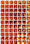 |
Fig. A.1. Cutouts of all 42 sources present in our final sample. ID 13 has already been shown in the main text. For IDs 1 to 14, 42, and 43, the sources belong to the first pointing and therefore are observed in ch3 and not ch4. For IDs 15 to 43, the objects are observed in ch4 and not in ch3; some of them are missing ch1 data because of the different image sizes (see the explanation in Sect. 2.2). These cutouts are 15″ × 15″. |
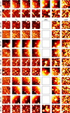 |
Fig. A.1. Continued. |
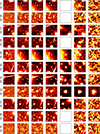 |
Fig. A.1. Continued. |
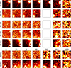 |
Fig. A.1. Continued. |
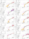 |
Fig. A.2. SED fits from Bagpipes in our main analyses. IDs 11, 13, 28, and 42 were already shown in the main text of the paper. The circles represent the photometric data points with S/N > 3, while the inverted triangles show upper limits at 3 σ. The different templates are explained in Sect. 4.1. |
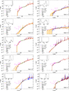 |
Fig. A.2. Continued. |
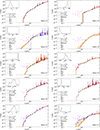 |
Fig. A.2. Continued. |
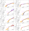 |
Fig. A.2. Continued. |
Main parameter output estimates retrieved by Bagpipes in our analyses, with the set-up presented in Table 4.
All Tables
Main parameter output estimates retrieved by Bagpipes in our analyses, with the set-up presented in Table 4.
All Figures
|
Fig. 1. Euclid red-green-blue image of the Perseus cluster made by combining the images taken through the three NISP filters. The solid coloured lines show the extent of the two Spitzer/IRAC datasets, with the cyan and magenta lines showing the extent of the first and second pointings, respectively. The images have been aligned with the WCS coordinate system, with north up and east to the left. In the low-right corner, a scale bar representing 5 arcmin is shown. |
| In the text | |
|
Fig. 2. Colour-magnitude (HE − ch2 versus ch2) distribution of the matched Euclid and Spitzer sample. The yellow stars show the objects that satisfy the HIERO colour criterion (shown as a dashed red line). The triangle symbols show lower limits for the HE-undetected objects, calculated using the 1σHE magnitude limit. The other points show the parent sample. |
| In the text | |
|
Fig. 3. Example multi-wavelength cutout of an object that was discarded due to an artefact in the VIS image. The cutout sizes are 15″ × 15″. |
| In the text | |
|
Fig. 4. Bagpipes fits to the SEDs for three representative objects, IDs 42, 28, and 11. The posterior PDF(z) are shown as insets. Photometric detections are shown by the coloured circles, and 3σ upper limits are plotted as triangles. The coloured lines show the three different fits described in the text. The PDF for ID 42 peaks at a low redshift, ID 28 is bimodal, and ID 11 has a single high-redshift peak, making it representative of the objects likely to be HIEROs. |
| In the text | |
|
Fig. 5. Properties of the HIEROs. Panel (a): Redshift versus stellar mass. The red circles show the most massive candidates, with stellar mass greater than 1011.7 M⊙. These objects are from here on defined as ‘over-massive’ and shown with the same symbol, i.e. red circles, in all other panels. The solid lines report the minimum observable stellar mass producing an IRAC ch2 magnitude of 22.7. All three curves represent star-forming galaxies, the green with an age between the redshift epoch and the burst peak of 200 Myr, the teal one 100 Myr, and the dark blue one 50 Myr. Panel (b): Redshift versus dust attenuation distribution. Panel (c): Dust attenuation versus stellar mass. The solid cyan line shows the relation from McLure et al. (2018), while the magenta line delimits the area identifying the so-called HELM galaxies (Bisigello et al. 2025). Different symbols report values from previous studies, as indicated in the legend. |
| In the text | |
|
Fig. 6. Different GSMFs: with the complete original sample (orange pentagons), with AGN candidates removed (empty orange stars), and with both the AGN candidates and over-massive objects removed, the most conservative case (filled orange stars). The comparison is shown with respect to the values found by Grazian et al. (2015, blue circles) and reported in Weaver et al. (2023, green triangles) and Weibel et al. (2024, magenta squares). The cyan crosses report the values found by Gottumukkala et al. (2024), who applied a similar selection to the JWST/CEERS dataset. |
| In the text | |
|
Fig. 7. Multi-wavelength cutouts of ID 13 with an estimated z ≈ 14. The available images are the Euclid bands IE, YE, JE, and HE and the Spitzer channels ch1, ch2, and ch3. The cutout size is 15″ × 15″. |
| In the text | |
|
Fig. 8. SED fits for ID 13: different SED fitting models found by Bagpipes (left) and the fit found by CIGALE (right). Both panels show photometric data points, both detections (circles) and upper limits (triangles). The PDF(z) are displayed in the insets. |
| In the text | |
|
Fig. A.1. Cutouts of all 42 sources present in our final sample. ID 13 has already been shown in the main text. For IDs 1 to 14, 42, and 43, the sources belong to the first pointing and therefore are observed in ch3 and not ch4. For IDs 15 to 43, the objects are observed in ch4 and not in ch3; some of them are missing ch1 data because of the different image sizes (see the explanation in Sect. 2.2). These cutouts are 15″ × 15″. |
| In the text | |
|
Fig. A.1. Continued. |
| In the text | |
|
Fig. A.1. Continued. |
| In the text | |
|
Fig. A.1. Continued. |
| In the text | |
|
Fig. A.2. SED fits from Bagpipes in our main analyses. IDs 11, 13, 28, and 42 were already shown in the main text of the paper. The circles represent the photometric data points with S/N > 3, while the inverted triangles show upper limits at 3 σ. The different templates are explained in Sect. 4.1. |
| In the text | |
|
Fig. A.2. Continued. |
| In the text | |
|
Fig. A.2. Continued. |
| In the text | |
|
Fig. A.2. Continued. |
| In the text | |
Current usage metrics show cumulative count of Article Views (full-text article views including HTML views, PDF and ePub downloads, according to the available data) and Abstracts Views on Vision4Press platform.
Data correspond to usage on the plateform after 2015. The current usage metrics is available 48-96 hours after online publication and is updated daily on week days.
Initial download of the metrics may take a while.