| Issue |
A&A
Volume 706, February 2026
|
|
|---|---|---|
| Article Number | A22 | |
| Number of page(s) | 11 | |
| Section | Numerical methods and codes | |
| DOI | https://doi.org/10.1051/0004-6361/202556460 | |
| Published online | 29 January 2026 | |
Using multi-task learning to determine gas-phase metallicity of star-forming galaxies
1
School of Computer and Information, Dezhou University,
Dezhou
253023,
China
2
School of Information and Control Engineering, Jilin University of Chemical Technology,
Jilin
132022,
China
★ Corresponding author: This email address is being protected from spambots. You need JavaScript enabled to view it.
Received:
17
July
2025
Accepted:
26
November
2025
Abstract
Aims. This study aimed to improve the estimation of the gas-phase metallicity of star-forming galaxies by using a multi-task learning approach that simultaneously performs gas-phase metallicity estimation and spectral classification of galaxies.
Methods. We propose a multi-task learning model to perform simultaneous gas-phase metallicity estimation and spectral classification of galaxies (MTLforGalSpecZ). The architecture is composed of three main components: (1) a shared feature extraction module, (2) a channel attention mechanism, and (3) two task-specific output heads. Specifically, the shared feature extraction module consists of stacked convolutional blocks that process spectroscopic inputs to extract global spectral features. These features are then passed to a channel attention mechanism, which adjusts the importance of each spectral channel. Finally, these features are fed into two separate output heads: a regression head to estimate the gas-phase metallicity and a classification head to determine the spectral class. The model is optimised using a combined loss function that includes both classification and regression losses. A conditional masking strategy is applied to the regression loss to ensure that metallicity estimation is performed only for star-forming galaxies.
Results. The model was trained on a dataset of approximately 100000 spectra, each labelled with a galaxy class, with gas-phase metallicity labels available for star-forming galaxies. On the test set, it achieves a prediction scatter of σ = 0.0374 for metallicity and a classification accuracy of 97.01%. Compared to running two independent single-task networks, MTLforGalSpecZ improves metallicity prediction performance by 30%, while also reducing total training time by 18.3% and inference time by 45.2%.
Key words: methods: data analysis / methods: statistical / techniques: spectroscopic / surveys
© The Authors 2026
 Open Access article, published by EDP Sciences, under the terms of the Creative Commons Attribution License (https://creativecommons.org/licenses/by/4.0), which permits unrestricted use, distribution, and reproduction in any medium, provided the original work is properly cited.
This article is published in open access under the Subscribe to Open model. This email address is being protected from spambots. You need JavaScript enabled to view it. to support open access publication.
1 Introduction
Star formation processes and gas physical properties are critical for understanding the mechanisms behind galaxy formation and evolution (Nagamine et al. 2016). Gas-phase metallicity is a key parameter in galaxy evolution, which influences the star formation rate, gas cooling processes, and supernova explosions (Simons et al. 2021; Maiolino & Mannucci 2019). High metal-licity indicates that a galaxy has undergone multiple episodes of star formation and supernova explosions, which enrich it with heavy elements (Boardman et al. 2023). Therefore, studying the gas-phase metallicity of star-forming galaxies is essential for understanding their chemical evolution and star formation history.
Traditional methods for estimating gas-phase metallicity include the Te method and the strong-line method. The Te method relies on auroral lines in the spectrum (e.g. [O III]λ4363, [NII]λ5755, and [SII]λ6312), which are sensitive to electron temperature (Garnett 1992; Pérez-Montero 2014). This method uses these lines to calculate the electron temperature and estimate the gas-phase metallicity. The strong-line method estimates metallicity using empirical relationships from diagnostic ratios based on strong emission lines in the spectrum, such as the R23 index (Pagel et al. 1979), defined as
![Mathematical equation: R_{23} = \frac{[\text{O\,II}]\,\lambda3727 + [\text{O\,III}]\,\lambda\lambda4959,5007}{\mathrm{H}\beta},](/articles/aa/full_html/2026/02/aa56460-25/aa56460-25-eq1.png) (1)
(1)
the N2 index (Denicoló et al. 2002),
![Mathematical equation: \mathrm{N2} = \log\left(\frac{[\text{N\,II}]\,\lambda6584}{\mathrm{H}\alpha}\right),](/articles/aa/full_html/2026/02/aa56460-25/aa56460-25-eq2.png) (2)
(2)
and the O3N2 index (Alloin et al. 1979),
![Mathematical equation: \mathrm{O3N2} = \log\left(\frac{[\text{O\,III}]\,\lambda5007/\mathrm{H}\beta}{[\text{N\,II}]\,\lambda6584/\mathrm{H}\alpha}\right).](/articles/aa/full_html/2026/02/aa56460-25/aa56460-25-eq3.png) (3)
(3)
These strong-line diagnostics are only calibrated for star-forming galaxies, although notable attempts at building calibrations for active galactic nuclei (AGNs), low-ionisation nuclear emissionline regions (LINERs), and other types do exist in the literature (Carvalho et al. 2020; Castro et al. 2017). Consequently, estimating the gas-phase metallicity generally requires first identifying star-forming galaxies within a spectral sample. The spectra of galaxies are traditionally classified into passive, star-forming, composite, or AGN categories using diagnostic diagrams such as the Baldwin-Phillips-Terlevich (BPT) diagram (Baldwin et al. 1981), which rely on ratios of strong emission lines, such as [NII]λ6584ZHα and [OIII]T5007ZHβ. Both gas-phase metal-licity estimation and spectral classification of galaxies require the measurement of specific emission lines. This process can be time-consuming, particularly when applied to large-scale spectroscopic surveys.
The rapid development of large-scale spectroscopic surveys, including the Sloan Digital Sky Survey (SDSS; York et al. 2000), the Large Sky Area Multi-Object Fiber Spectroscopic Telescope (LAMOST; Luo et al. 2015; Cui et al. 2012), and the Dark Energy Spectroscopic Instrument (DESI; DESI Collaboration 2025), has ushered astronomical spectroscopy into the big data era. Machine learning (ML) and deep learning (DL) techniques have proven highly effective in extracting meaningful features from spectral data. In galaxy parameter prediction, Ho (2019) used artificial neural networks (ANN) to estimate gas-phase metallicity in HII regions using 16 strong emission-line features, and Wang et al. (2024) used CNN to predict stellar population parameters of galaxies with spectra. In spectral classification, Chen (2021) used 1D CNN to distinguish Seyfert 1.9 spectra from Seyfert 2 galaxies, Wang et al. (2023) used spectral features around key emission lines to classify emissionline galaxies into star-forming, composite, LINER, and Seyfert classes based on ML models, and Wu et al. (2024) used CNN to classify galaxy spectra into star-forming, composite, AGN, and normal categories, and to analyse spectral features. Overall, gas-phase metallicity estimation and spectral classification of galaxies are based on spectral data and often rely on similar spectral features. However, most existing studies treat these tasks separately, which may lead to redundant feature extraction, increased computational cost, and longer processing times.
Multi-task learning (MTL) has gained considerable attention as a strategy to improve predictive performance and model efficiency by jointly learning multiple related tasks within a single model (Caruana 1997; Ruder 2017; Crawshaw 2020). Recent studies in astronomy demonstrate the effectiveness of MTL. Cabayol et al. (2023) used an MTL neural network to improve broadband photometric redshift estimates by simultaneously predicting broadband photometric redshifts and narrow-band photometry, where narrow-band data were only required in the training field. This approach enables improved photometric redshift predictions for galaxies without narrow-band photometry in the wide field. Ginolfi et al. (2025) utilised a multi-task CNN model to simultaneously infer redshift and key galaxy properties, such as stellar mass and star formation rate. These results demonstrate the potential of MTL frameworks for applications across multiple related astrophysical tasks.
In this work, we propose a multi-task learning framework to improve gas-phase metallicity estimation by jointly performing gas-phase metallicity estimation and spectral classification of galaxies (MTLforGalSpecZ). By integrating both tasks into a unified framework, the model can effectively share spectral features between tasks, improving learning efficiency and predictive accuracy. The structure of this paper is as follows. Section 2 describes the data selection and pre-processing steps. Section 3 presents the architecture and training details of the MTLfor-GalSpecZ model. Section 4 evaluates the model’s performance. Section 5 summarises the paper and outlines directions for future work.
2 Data
This section provides a description of the data used to train and evaluate the MTLforGalSpecZ model. Specifically, Sect. 2.1 details the data selection process, and Sect. 2.2 describes the preprocessing steps applied to prepare the spectra for input into the model.
2.1 Data selection
This study uses galaxy spectra from the SDSS Data Release 15 (DR15; Aguado et al. 2019) to construct a dataset for MTLforGalSpecZ. The SDSS DR15 contains 2779 151 galaxy spectra, each covering 3800-9200 Å with a spectral resolution of R ~ 2000.
To ensure data quality, we filtered the raw spectra by selecting galaxies with redshifts between 0.002 and 0.3, ensuring that key emission lines (such as Hß, [OIII], [NII], and Hα) fall within the spectral observation range. We used only spectra with zWarning = 0 to ensure reliable spectroscopic redshifts. In addition, we included only spectra with a signal-to-noise ratio in the r-band (S/Nr) of at least five to ensure data quality for reliable analysis.
After applying these filters, approximately 1 million spectra remained. To obtain spectral classification of galaxies and gas-phase metallicity labels, we used two value-added catalogues: galSpecExtra and emissionLinesPort. The galSpecExtra catalogue provides both spectral classification and gas-phase metallicity values, while the emissionLinesPort catalogue provides spectral classes. These catalogues are provided by the Max Planck Institute for Astrophysics and Johns Hopkins University (MPA-JHU)1, and the Portsmouth group (Maraston et al. 2013), respectively.
To ensure consistent and reliable class labels, we used both catalogues. The galSpecExtra catalogue, based on SDSS DR8 spectra, derives emission-line fluxes by fitting the stellar continuum with a non-negative least-squares routine (Lawson & Hanson 1974) and then applies Gaussian fits to the emission lines following Tremonti et al. (2004), with classifications assigned on the BPT diagram following Brinchmann et al. (2004). In contrast, the emissionLinesPort catalogue is based on SDSS DR12 spectra and measures emission lines using the penalized PixelFitting (pPXF) and Gas AND Absorption Line Fitting (GANDALF) pipelines (Cappellari & Emsellem 2004; Sarzi et al. 2006), with classifications following the schemes of Kauffmann et al. (2003), Kewley et al. (2001), and Schawinski et al. (2007). As the two catalogues are derived from different data releases and use different emission-line measurement methods, their classifications show some differences. To minimise possible systematic uncertainties from a single method, we cross-matched the two catalogues and retained only galaxies whose classes agree in both. The final class labels were then mapped into the four categories used in this study: passive galaxy, star-forming galaxy, composite galaxy, and AGN, as detailed in Table 1.
For gas-phase metallicity labels, we used the oh_p50 field from the galSpecExtra catalogue, which represents the median value of gas-phase metallicity expressed in units of 12 + log(O/H). These values were derived using the methodology described in Tremonti et al. (2004), which employs Bayesian inference combined with a large grid of photoionisation models to fit multiple strong emission lines. Although we adopted the Tremonti calibration in this work, other strong-line metallicity calibrations would have been equally suitable. To ensure reliable metallicity data, we excluded star-forming galaxies with invalid values (i.e. oh_p50 = −9999).
After applying the above steps, approximately 321 000 galaxies remained. To reduce computational cost, we selected 100 000 galaxies as our model’s dataset, randomly sampling 25 000 galaxies from each of the four classes. Among them, the 25 000 star-forming galaxies have valid gas-phase metallicity labels. Figure 1 shows the distributions of redshift, S/Nr, and magnitude (petroMag_r) between the full filtered 321 000-galaxy dataset and the selected 100 000 dataset. The close agreement between the two curves in all three parameters indicates that the randomly selected subset provides a representative sample of the full dataset. The redshift values are mostly within [0.02, 0.15], the S/Nr ranges from 5 to 30, and the petroMag_r values cluster between 16 and 18.
Mapping of galaxy classes between the galSpecExtra and emissionLinesPort catalogues.
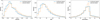 |
Fig. 1 Distributions of redshift, signal-to-noise ratio in the r-band (S/Nr), and Petrosian magnitude in the r-band (petroMag_r). Solid blue lines represent the main filtered dataset, and dashed yellow lines show the selected subset. |
2.2 Data pre-processing
To ensure the consistency of the input spectra for MTLforGal-SpecZ, we performed spectral interpolation and standardisation on our dataset. Each spectrum was linearly interpolated at 1 Å intervals within the wavelength range 3840-9000 Å, resulting in a total of 5161 pixels. This wavelength range was chosen because, although the nominal coverage of SDSS spectra is 3800-9200 Å, not all spectra actually span this full range. Setting the blue-end limit to 3800 Å would exclude 82.7% of the spectra in our sample, while adopting 3830 Å would still remove about 2.2%. In contrast, choosing 3840 Å results in the exclusion of only 0.7%, allowing us to preserve a larger portion of the dataset. For the red limit, we adopted 9000 Å to ensure the inclusion of key emission lines such as Hα and [N II]λ6584, even for galaxies at the highest redshift (z = 0.3) in our sample.
After interpolation, each spectrum was normalised by dividing its flux values by the mean flux of that spectrum. Specifically, the flux of a spectrum is represented as an m-dimensional vector, denoted by F = (f1, f2,..., fm)T. The standardised flux F′ is obtained by dividing the original flux by the mean value across all flux points, as
 (4)
(4)
Here, m is the number of wavelength points in the spectrum and  denotes the mean flux of the original spectrum. After normalisation, each spectrum has a mean flux of 1.
Through these pre-processing steps, we ensured that the input data were not only dimensionally consistent but also numerically stable, providing a reliable foundation for training MTLforGalSpecZ.
3 Methodology
This section introduces the design and training of MTLfor-GalSpecZ. The model was developed to perform two tasks simultaneously: gas-phase metallicity estimation and spectral classification of galaxies. Section 3.1 details the architecture of the MTLforGalSpecZ, Sect. 3.2 formulates the multi-task loss function, and Sect. 3.3 describes the training strategy.
3.1 Multi-task model architecture
The MTLforGalSpecZ model adopts a multi-task learning framework to simultaneously learn from 1D galaxy spectra for both gas-phase metallicity estimation and spectral classification tasks. The overall model architecture and training flow are shown in Fig. 2. The architecture is composed of three main components: (1) a shared feature extraction module built with stacked convolutional blocks, (2) a channel attention mechanism, and (3) two task-specific output heads for gas-phase metallicity regression and spectral classification.
- (1)
Shared feature extraction module. The model input consists of pre-processed spectra, each containing 5161 pixels. The shared feature extraction module is composed of five convolutional blocks. Each block contains two convolutional layers with rectified linear unit (ReLU) activation functions followed by a max-pooling layer. Each convolutional layer is labelled Conv1Dxx, where xx indicates the progressively increasing number of channels (16, 32, 64, 128, and 256) for extracting increasingly complex features. The kernel size for all convolutional layers is set to three, with a stride of one. The pooling window size for max-pooling layers is three, with a stride of three.
- (2)
Channel attention mechanism. To enhance the model’s ability to focus on task-relevant information, we introduced a channel attention module inspired by the squeeze-and-excitation (SE) mechanism (Hu et al. 2020). This module first applies global average pooling (GAP) to compress each channel into a single representative value, which is then processed by two 1D convolutional layers (kernel size 1) with 16 and 256 output channels, followed by ReLU and sigmoid activations, respectively. The resulting attention weights are applied to the original feature map through channel-wise multiplication, allowing the model to focus on task-relevant channels.
- (3)
Task-specific output heads. Following the attention-enhanced feature map, a global average pooling layer reduces the spatial dimension, and the resulting vector is passed to two separate output branches. The classification output head consists of a flattening layer, dropout, and three fully connected (FC) layers with decreasing dimensions (128 → 64 → num_classes) and ReLU activations, yielding class probabilities via softmax for spectral classification. The regression output head shares a similar structure, but outputs predicted gas-phase metallicity.
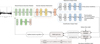 |
Fig. 2 Architecture and training workflow of MTLforGalSpecZ. The model comprises three main components: (1) a shared feature extraction module with multiple convolutional blocks to process input spectra; (2) a channel attention mechanism to enhance task-relevant features; and (3) two task-specific output heads—one for spectral classification of galaxies and the other for gas-phase metallicity regression. Training is guided by a joint loss function that combines focal loss for classification and masked mean absolute error (MAE) loss for regression, enabling end-to-end multi-task optimisation. |
3.2 Multi-task loss function
To enable the simultaneous optimisation of gas-phase metallic-ity prediction and spectral classification of galaxies, we adopted a multi-task loss function that combines two task-specific objectives into a single loss function. The total loss is defined as a weighted sum of the classification and regression losses:
 (5)
(5)
where Lclass and Lregress represent the classification and regression losses, respectively. The weights λ1 and λ2 control the relative importance of each task. They can be manually specified or dynamically adjusted during training to adapt to the changing learning difficulty of each task. In our experiments, we adopted dynamic weights to balance the two tasks during training; further details are provided in Sect. 3.3.
The classification branch aims to identify the galaxy class from four categories: passive, star-forming, composite, and AGN. To supervise this task, we used focal loss (Lin et al. 2020). The classification loss (Lclass) is defined as
 (6)
(6)
where N is the number of samples, C is the number of classes, yi,c denotes whether class c is the correct label for sample i, and pi,c is the predicted probability that sample i belongs to class c. The modulating factor (1 - pi,c)γ reduces the loss contribution from easy examples, while the weighting factor αc balances the importance of different classes. The parameters γ > 0 and 0 ≤ αc ≤ 1 control the degree of focusing and class weighting, respectively. In this study, we set α = 0.25 to reflect that all four categories are equally important in our classification task. We used γ = 2.0, the default value recommended by Lin et al. (2020).
The regression branch estimates the gas-phase metallicity only for star-forming galaxies. To prevent interference from nonstar-forming galaxies, we applied a conditional masking mechanism. Specifically, only samples classified as star-forming galaxies contribute to the regression loss. The conditional masked loss is defined as
 (7)
(7)
where ypred,i and ytrue,i denote the predicted and true gas-phase metallicity of the i-th sample, respectively. We define the mask variable Mi as

This masking strategy ensures that the regression branch focuses on star-forming galaxies, thereby improving the accuracy and robustness of the gas-phase metallicity predictions.
3.3 Multi-task model training
We trained and evaluated the MTLforGalSpecZ model using our full GPU-accelerated pipeline. All training and evaluation was conducted on an NVIDIA GeForce RTX 3080 Ti GPU (12 GB) paired with an Intel 11th Gen Core i7-11700F CPU. The software environment includes Python 3.11, NumPy 2.2.2, Pandas 2.2.3, scikit-learn 1.6.1, PyTorch 2.3.1, and CUDA 12.1.
We describe the training process from the following four aspects:
- (1)
Dataset split. We trained the MTLforGalSpecZ model using the pre-processed dataset described in Sect. 2.2. This dataset contains approximately 100000 spectra, each labelled with a galaxy class. Among these, 25 000 star-forming galaxies have gas-phase metallicity labels. The dataset was randomly divided into training, validation, and test sets with a ratio of 6:2:2. The distributions of the training, validation, and test sets for both the regression and classification labels. Panel a shows the distribution of galaxy classes across the three subsets, covering four classes: passive, star-forming, composite, and AGN. The proportions of each galaxy class are consistently maintained across the training, validation, and test sets, which is essential for unbiased model training and fair performance evaluation. Panel b shows that the distributions of gas-phase metallicity values in the three subsets are highly consistent, which provides reliable support for both learning and generalisation.
- (2)
Loss function and dynamic weighting strategy. The MTLforGalSpecZ model was trained using the combined classification (Eq. (6)) and regression (Eq. (7)) loss function described in Sect. 3.2. To dynamically balance the optimisation between the classification and regression tasks, we adopted the dynamic weight average (DWA) strategy proposed by Liu et al. (2019). In this method, task weights λk (t) for task k are updated at the end of each epoch based on the relative changes in recent task losses, as shown in Eq. (8). Here, k = 1 corresponds to the classification task and k = 2 to the regression task.
 (8)
where K is the number of tasks (K = 2 in our experiments) and T is a temperature coefficient that controls the smoothness of the task weighting distribution. A higher T leads to more balanced weights across tasks, while a lower T increases the sensitivity to the relative descent rate. In our experiments, we set T = 1 to make the weighting more responsive to task differences.
(8)
where K is the number of tasks (K = 2 in our experiments) and T is a temperature coefficient that controls the smoothness of the task weighting distribution. A higher T leads to more balanced weights across tasks, while a lower T increases the sensitivity to the relative descent rate. In our experiments, we set T = 1 to make the weighting more responsive to task differences.The wk(t) represents the relative loss descent rate for task k at epoch t, calculated as the ratio of the average loss in epoch t - 1 to that in epoch t - 2:
 (9)
where Lk(t) denotes the average loss of task k in epoch t. For t = 1, 2, we initialised wk(t) = 1. This formulation captures how fast each task is learning. Tasks with slower descent are assigned higher weights in the following epoch.
(9)
where Lk(t) denotes the average loss of task k in epoch t. For t = 1, 2, we initialised wk(t) = 1. This formulation captures how fast each task is learning. Tasks with slower descent are assigned higher weights in the following epoch. - (3)
Hyperparameters. The Adam optimiser was used with an initial learning rate of 0.001. Adam effectively improves the model’s convergence speed and stability. To further optimise learning rate adjustments during training, we employed a ReduceLROnPlateau2 scheduler. This scheduler reduces the learning rate by a factor of ten when the validation loss does not show an improvement for ten consecutive epochs, helping the model to stabilise convergence and refine its optimisation near the global optimum.
- (4)
Training procedure. During training, the spectra and their corresponding labels were fed into the MTLforGalSpecZ model in batches of 128. The model parameters were updated using the back-propagation algorithm in each epoch to minimise the loss function. The training process spans 100 epochs. Figure 4 shows that the loss decreases steadily for both training and validation sets, with minimal difference between the two, indicating good model performance. Figure 5 shows the evolution of the task weights assigned by the DWA strategy during training. The classification and regression task weights exhibit fluctuations during the early training stages. As training progresses, after approximately 60 epochs, both weights begin to stabilise and converge towards one. This convergence suggests that the model has learned to treat both tasks with comparable importance, indicating a balanced optimisation of the two tasks.
4 Results and discussion
This section presents an evaluation of MTLforGalSpecZ’s performance on the test set for both gas-phase metallicity regression and galaxy spectral classification. The evaluation comprises five parts. Section 4.1 introduces the metrics used to quantify the performance of regression and classification. Section 4.2 evaluates the performance of MTLforGalSpecZ. Section 4.3 compares MTLforGalSpecZ with single-task baselines for classification and regression. Section 4.4 evaluates MTLforGalSpecZ applied to DESI spectra. Finally, Sect. 4.5 explores the model’s ability to recover the mass-metallicity relation (MZR).
4.1 Evaluation metrics
To assess the performance of MTLforGalSpecZ, we adopted a set of evaluation metrics for both the regression and classification tasks.
- (1)
Gas-phase metallicity regression. We evaluated the regression task using the mean squared error (MSE), mean absolute error (MAE), standard deviation (SD) of the prediction errors, and the coefficient of determination R2. The MSE and MAE measure the magnitude of the prediction errors, with the MSE being more sensitive to large deviations. The SD reflects the variability of the error distribution around its mean, and the R2 score measures how well the model’s predictions account for the variance of the true values. The mathematical definitions of these metrics are as follows:
 (10)
(10)
 (11)
(11)
 (12)
(12)
 (13)
where ypred,i and ytrue,i denote the predicted and true values of the i-th sample, ∆̄ represents the mean value of the prediction errors (ypred - ytrue), and ȳ is the mean of all true values.
(13)
where ypred,i and ytrue,i denote the predicted and true values of the i-th sample, ∆̄ represents the mean value of the prediction errors (ypred - ytrue), and ȳ is the mean of all true values. - (2)
Spectral classification of galaxies. We report four metrics: accuracy, precision, recall, and F1 score. Accuracy measures the proportion of correctly classified samples among all samples. Precision quantifies the proportion of true positives among all positive predictions, while recall assesses the proportion of actual positives correctly identified. The F1 score provides a harmonic mean of precision and recall. The mathematical definitions of these metrics are as follows:
 (14)
(14)
 (15)
(15)
 (16)
(16)
 (17)
here, TP (true positives) is the number of samples correctly predicted as a given class, FP (false positives) is the number of samples incorrectly predicted as that class, TN (true negatives) is the number of samples correctly predicted as not belonging to that class, and FN (false negatives) is the number of samples belonging to that class but incorrectly predicted as another class.
(17)
here, TP (true positives) is the number of samples correctly predicted as a given class, FP (false positives) is the number of samples incorrectly predicted as that class, TN (true negatives) is the number of samples correctly predicted as not belonging to that class, and FN (false negatives) is the number of samples belonging to that class but incorrectly predicted as another class.
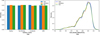 |
Fig. 3 Distributions of training, validation, and test sets. (a) Galaxy classes used in the classification task. (b) Gas-phase metallicity for star-forming galaxies used in the regression task. |
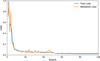 |
Fig. 4 Training and validation loss curves over 100 epochs. The blue line represents the training loss, while the yellow line represents the validation loss. |
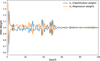 |
Fig. 5 Evolution of DWA weights for the classification and regression tasks over 100 training epochs. The blue line represents the weight for the spectral classification task (λ1), and the yellow line represents the weight for the gas-phase metallicity regression task (λ2). |
4.2 Model evaluation
In this section, we present three experiments to evaluate the performance of MTLforGalSpecZ. First, we assess its classification and regression performance on the test set in Sect. 4.2.1. Second, we quantify the contribution of the channel attention mechanism in Sect. 4.2.2. Third, we investigate the impact of redshift in Sect. 4.2.3. Finally, we examine the effect of the variations in the signal-to-noise ratio in Sect. 4.2.4.
4.2.1 Evaluation of MTLforGalSpecZ predictions on the test set
We evaluated the performance of MTLforGalSpecZ on the test set, assessing its ability to predict gas-phase metallicity and classify galaxy spectra.
- (1)
Gas-phase metallicity regression. Fig. 6 shows a scatter density plot comparing the predicted gas-phase metallicity (Zpred) with the true values (Ztrue) for star-forming galaxies. In the main panel, the solid black line represents the ideal 1:1 relation, while the red line traces the median values of Zpred. The dashed purple lines indicate the 1σ scatter around the median. The red median line closely follows the 1:1 reference, indicating high predictive accuracy. We observe slight deviations at the lower (<8.5) and upper (>9.2) ends of the metallicity range, likely due to reduced sample counts in these regions (as shown in Fig. 3b). The key metrics are shown in the top-left of the main panel: the prediction bias (mean residual) is μ = 0.0026 dex, with MSE = 0.0014, MAE = 0.0223, R2 = 0.9730, and SD = 0.0374 dex, indicating excellent predictive performance. The top panel shows the residual distribution (∆Z = Zpred - Ztrue), which is approximately symmetric and concentrated within the range −0.05 to +0.05 dex, suggesting minimal systematic bias.
In addition, we further quantified the predictive uncertainty of our metallicity regression branch using the Monte Carlo (MC) dropout method. Specifically, we performed 100 stochastic forward passes for each star-forming galaxy and computed the standard deviation of the predicted metallicity values, which is treated as the 1σ uncertainty. The results are shown in Fig. 7. The dots in the figure represent the mean value of the 1 σ uncertainty within each metallicity interval, while the vertical line segments indicate the standard deviation of the uncertainty within each interval. The predictive uncertainty reaches its maximum at the low-metallicity end (Zpred ~ 8.0), with a value of approximately 0.05 dex. As the metallicity increases, the uncertainty gradually decreases, reaching a minimum of approximately 0.01 dex around Zpred - 9.0. This trend can be explained by the distribution of samples: as shown in Fig. 6, the low-metallicity region (< 8.5) contains fewer samples and exhibits a larger scatter between predicted and true values, resulting in higher predictive uncertainty. In contrast, in the high-metallicity regime, where most samples are concentrated and the scatter between prediction and truth is smaller, the uncertainty is correspondingly reduced.
- (2)
Spectral classification of galaxies. The model achieves an overall classification accuracy of 97.01% across the four galaxy types. The corresponding precision, recall, and F1 score are also all 97.01%, indicating reliable classification performance (see Table 4 for a detailed summary of these metrics). The confusion matrix in Fig. 8 provides a detailed view of the classification results. The model demonstrates particularly high accuracy for passive galaxies (98.9%) and star-forming galaxies (98.3%), with only a small number of misclassifications. In contrast, the composite (95.3%) and AGN (95.4%) classes exhibit relatively higher misclassification rates. Composite galaxies have spectral features similar to both star-forming and AGN galaxies, making them easier to confuse. Despite this, the total number of misclassified samples remains small, highlighting the overall robustness of the model’s predictions.
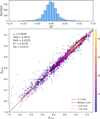 |
Fig. 6 Comparison of gas-phase metallicity predictions (Zpred) from the MTLforGalSpecZ model with true values (Ztrue) for star-forming galaxies. The main panel shows a scatter density plot of gas-phase metallicity: the solid black line indicates the 1:1 relation, the red line shows the median predicted metallicity against the true value, and the dashed purple lines represent the 1σ scatter around the median. The top panel shows the residual distribution (∆Z = Zpred - Ztrue ). |
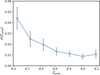 |
Fig. 7 Uncertainty estimation of the metallicity regression branch using MC Dropout. The black circles represent the mean 1σ uncertainty (σ(Zpred)) within each bin of predicted metallicity (Zpred), and the vertical bars indicate the standard deviation of the uncertainty values within each bin. |
4.2.2 Impact of the channel attention mechanism
To evaluate the contribution of the channel attention module, we conducted an experiment comparing the model with attention to a baseline model without this component. The results are summarised in Table 2.
For the classification task, the incorporation of channel attention improves all metrics, with accuracy increasing from 95.61% to 97.01%. For the regression task, the inclusion of channel attention leads to consistent improvements, reducing the MSE and MAE (0.0025 → 0.0014 and 0.0334 → 0.0223) and decreasing the standard deviation by about 20% (0.0468 → 0.0374). These results demonstrate that incorporating the channel attention mechanism enhances the overall performance of the model, especially for the regression task.
4.2.3 Evaluation of MTLforGalSpecZ at different redshifts
Redshift is a key parameter in astronomical observations. Because the spectra in our dataset were not redshifted to rest wavelengths, it is important to assess how well the trained model generalises across different redshifts. To assess the impact of redshift on our model, we divided the data into several redshift intervals: [0.0,0.04), [0.04,0.08), [0.08,0.12), [0.12,0.15), [0.15, 0.20), and [0.20, 0.30).
- (1)
Gas-phase metallicity regression. In each redshift bin, we calculated the SD between the values of Zpred and Ztrue. As shown by the dashed yellow line in Fig. 9a, the gas-phase metal-licity prediction error remains low, stabilising at approximately 0.04 dex for redshifts in the range 0.05-0.3. At lower redshifts, the error increases and reaches approximately 0.06 dex. This performance degradation can be attributed to the fact that, for z < 0.03, the [OII]λ3727 emission line falls outside the adopted wavelength range.
- (2)
Spectral classification of galaxies. We compute the classification accuracy within each redshift interval. As shown by the solid blue line in Fig. 9a, the classification accuracy remains consistently high (above 96%) across all redshift bins, indicating that the model performs robustly over the entire redshift range. Overall, the MTLforGalSpecZ model demonstrates robust generalisation across a wide redshift range, maintaining high classification accuracy and low regression error.
Performance comparison of models with and without channel attention.
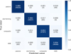 |
Fig. 8 Confusion matrix comparing spectral classification results from MTLforGalSpecZ with the true labels. The colour intensity and numerical values within each cell indicate the proportion of predictions for each class. |
4.2.4 Evaluation of MTLforGalSpecZ at different S/Nr levels
The signal-to-noise ratio may affect the predictive accuracy of MTLforGalSpecZ. To assess the model’s performance across different S/Nr levels, we divided the data into several S/Nr intervals: [5, 10), [10, 15), [15, 20), [20, 25), [25, 30), and [30, 100).
- (1)
Gas-phase metallicity regression. We calculated the SD between predicted and true gas-phase metallicity values (Zpred -Ztrue) in each S/Nr bin, as illustrated by the dashed yellow line in Fig. 9b. The largest prediction error occurs in the lowest S/Nr bin ([5, 10)), reaching approximately 0.06 dex. As the S/Nr increases, the SD decreases, reaching about 0.02 dex for the highest-quality spectra (S /Nr ≥ 30). These results confirm that the performance of the metallicity regression improves with increasing data quality, as expected.
- (2)
Spectral classification of galaxies. We computed the classification accuracy within each S/Nr bin. As shown by the solid blue line in Fig. 9b, the classification accuracy remains stable at around 97% for S/Nr values in the range[5, 30). However, when the S/Nr exceeds 30, the classification accuracy shows a slight decrease, falling to around 96%. This decrease may be attributed to a severe class imbalance in the high S/Nr interval. Specifically, in the S /Nr ≥ 30 bin, AGN galaxies account for 53.4% and composite galaxies for 30.7%, whereas star-forming and passive galaxies represent only 6.7% and 9.2%, respectively. This imbalance likely causes the model to overfit the dominant AGN class, resulting in degraded classification performance in this S/Nr range.
Overall, MTLforGalSpecZ performs well across different S/Nr intervals, achieving reliable results in both galaxy gasphase metallicity prediction and galaxy classification.
Comparison of regression performance between the multi-task and single-task regression models.
4.3 Comparison with single-task baselines
In this section, we compare MTLforGalSpecZ with its singletask counterparts in terms of predictive performance (Sect. 4.3.1) and computational efficiency (Sect. 4.3.2) under the same experimental settings.
4.3.1 Comparison of model performance: multi-task vs. single-task
We compared the performance of MTLforGalSpecZ with its single-task counterparts for both gas-phase metallicity regression and spectral classification tasks.
- (1)
Gas-phase metallicity regression. We compared the regression performance of MTLforGalSpecZ with that of a single-task regression model. The single-task regression model shares the same backbone architecture as MTLforGalSpecZ, with the classification head removed. For the training and evaluation dataset, we extracted approximately 25 000 star-forming galaxies from the sample of about 100000 spectra. The only difference in the training procedure lies in the loss function, where the multi-task loss is replaced by a mean absolute error loss. Table 3 presents the regression results for both models. MTLforGalSpecZ achieves a lower MSE (0.0014 vs. 0.0028), a lower MAE (0.0223 vs. 0.0302), and a higher R2 score (0.9730 vs. 0.9447). The SD of the prediction is reduced from 0.0532 to 0.0374, corresponding to a relative improvement of approximately 30%. These results demonstrate that the regression performance of MTLforGalSpecZ is significantly better than that of the single-task regression model.
- (2)
Spectral classification of galaxies. We evaluated the classification performance of MTLforGalSpecZ against a single-task classification model that shares the same backbone architecture. The only difference is that the single-task model removes the regression head, focusing solely on classification. The training procedure remains consistent between the two models, with the multi-task loss in MTLforGalSpecZ replaced by a focal loss for the single-task classifier. Table 4 presents the classification results in terms of precision, recall, F1 score, and accuracy. Overall, the multi-task model slightly outperforms the singletask model across all metrics. Specifically, it achieves an overall accuracy of 97.01%, compared to 96.80% for the single-task model.
In summary, the results of the comparison across both tasks demonstrate the advantages of multi-task learning: spectral classification helps improve metallicity estimation, while metallicity prediction contributes little to classification accuracy.
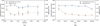 |
Fig. 9 Model performance across different redshift (a) and signal-to-noise ratio in the r-band (S/Nr) intervals (b). In each panel, the solid blue line represents spectral classification accuracy, while the dashed yellow line indicates the standard deviation (σ) of gas-phase metallicity predictions (∆ = Zpred - Ztrue). Error bars in each interval denote the standard deviation of the prediction error, and black circles indicate the median standard deviation within each bin. |
Comparison of classification performance between the multitask and single-task classification models.
4.3.2 Comparison of computational efficiency: Multi-task versus single-task
In addition to predictive performance, we assessed the computational efficiency of MTLforGalSpecZ relative to its single-task counterparts. Specifically, we evaluated the total training and inference times under identical hardware conditions. The comparative results are presented in Table 5.
Our goal was to obtain the gas-phase metallicity of starforming galaxies. The multi-task model performs both spectral classification of galaxies and metallicity prediction in a single training process, requiring 703 s. In contrast, the single-task approach involves first training a classification model to identify star-forming galaxies (649 s) and then training a regression model to predict their gas-phase metallicity (211 s), resulting in a combined training time of 860 s. This represents an 18.3% reduction in total training time for the multi-task approach.
For inference, we used the test set as input to the trained models and measure the average time taken per spectrum. On average, the multi-task model predicts both the galaxy class and the gas-phase metallicity in 1.55 ms per sample. By contrast, in the single-task setting, predicting both outputs requires sequentially applying the classification and regression models, with a combined average of 2.83 ms per sample (1.45 + 1.38 ms). This demonstrates that the multi-task model is approximately 45.2% faster than the combined single-task pipeline.
These findings further demonstrate that the multi-task model not only achieves good predictive performance, but also makes efficient use of computational resources.
Comparison of training and inference time between the multitask and single-task models.
4.4 Evaluation of the MTLforGalSpecZ model applied to DESI spectra
To evaluate the generalisation performance of the proposed model beyond the SDSS domain, we further applied the trained MTLforGalSpecZ model to the DESI Early Data Release (EDR) spectra (DESI Collaboration 2024a,b).
We cross-matched the ~321 000 SDSS galaxies with class and gas-phase metallicity labels described in Sect. 2.1 against the DESI EDR catalogue, yielding ~8900 paired spectra. Each DESI spectrum was processed following the same pre-processing pipeline described in Sect. 2.2, and the resulting spectra were subsequently fed into the trained MTLforGalSpecZ model to predict both the galaxy class and gas-phase metallicity. The predicted results were then compared with the corresponding SDSS reference values, as summarised in Table 6.
For the regression of gas-phase metallicity in star-forming galaxies, the model achieves an SD of 0.1125, an MSE of 0.0153, an MAE of 0.0869, and an R2 score of 0.6920. In the galaxy classification task, it achieves an overall accuracy of 79.47%, a precision of 86.19%, a recall of 79.47%, and an F1 score of 81.12%. Although these indices are lower than those obtained on the SDSS test set (see Sect. 4.2.1), they demonstrate that the MTLforGalSpecZ model retains predictive capability when applied to DESI spectra. The degradation reflects domain shifts between SDSS and DESI, primarily due to differences in instrumental configurations, spectral resolution, and flux calibration, which result in variations in spectral features. To further enhance performance on DESI spectra, fine-tuning our MTLforGalSpecZ model with a subset of DESI data or retraining it within the DESI domain could be effective strategies, which we plan to explore in future work.
Performance of the MTLforGalSpecZ model applied to DESI EDR spectra.
4.5 Recovering the mass-metallicity relation with MTLforGalSpecZ
The mass-metallicity relation (MZR) is a crucial empirical relationship in astronomy that describes the interaction between stellar mass and gas-phase metallicity in galaxies (Kewley & Ellison 2008; Gillman et al. 2021; Looser et al. 2024). Stellar mass reflects the history and scale of star formation within a galaxy, while gas-phase metallicity traces the accumulation of heavy elements and the chemical evolution of the galaxy. Investigating the MZR provides insight into the fundamental physical processes of galaxy formation and evolution. Following the empirical relation established by Tremonti et al. (2004), which is valid for stellar masses in the range 8.5 < log(M*/M⊙) < 11.5, we compared our predicted MZR with their results.
In this study, we used the test set to analyse the relationship between gas-phase metallicity and stellar mass. The gas-phase metallicity was predicted by MTLforGalSpecZ, while the stellar mass values were obtained from the lgm_fib_p50 parameter in the galSpecExtra catalogue. We restricted the stellar mass range in the test set to 8.5 < log(M*/M⊙) < 11.5, and plotted the predicted gas-phase metallicity (Zpred) as a function of stellar mass (log(M*/M⊙)), as shown in Fig. 10. The solid red line indicates the fitted relation, described by Eq. (18):
![Mathematical equation: \begin{aligned} 12 + \log(O/H) ={} & 0.217 + 1.613 \times \log(M_* / M_\odot) \\ & - 0.07307 \times [\log(M_* / M_\odot)]^2 \end{aligned},](/articles/aa/full_html/2026/02/aa56460-25/aa56460-25-eq20.png) (18)
(18)
where 12 + log(O/H) represents the gas-phase metallicity and log(M*/M⊙) is the logarithm of the stellar mass (M*) relative to the solar mass (M⊙).
In Fig. 10, the solid red line represents the median gas-phase metallicity predicted by MTLforGalSpecZ, while the dashed red lines indicate the ±σ deviation, which is approximately ±0.1 dex. In contrast, the solid and dashed black lines denote the empirical median MZR and its ±σ range as proposed by Tremonti et al. (2004). The results demonstrate that the MTLforGalSpecZ predicted MZR is consistent with the empirical MZR across most of the range, particularly within the main mass interval.
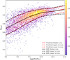 |
Fig. 10 Recovery of the mass-metallicity relation (MZR) predicted by the MTLforGalSpecZ. The solid red line represents the median gasphase metallicity predicted by the MTLforGalSpecZ, and the dashed red lines indicate the ±1σ deviation, approximately ±0.1 dex. The solid and dashed black lines represent the median empirical MZR and its ±1σ range proposed by Tremonti et al. (2004). |
5 Summary
This study presents a multi-task learning approach to improve gas-phase metallicity predictions for star-forming galaxies by simultaneously performing gas-phase metallicity estimation and spectral classification. The proposed model integrates convolutional feature extraction, a channel attention mechanism, and task-specific branches for gas-phase metallicity regression and spectral classification (passive, star-forming, composite, and AGN). Using approximately 100000 pre-processed galaxy spectra, the standard deviation of the gas-phase metallicity predictions for star-forming galaxies is 0.0374 dex.
To evaluate the model performance, we assessed it from the following perspectives:
Prediction performance: the model achieves highly accurate results, with gas-phase metallicity predictions showing low bias (0.0026 dex) and low scatter (0.0374 dex). Classification metrics including accuracy, precision, recall, and F1 score all reach 97.01%, reflecting strong performance across tasks.
Evaluation across redshift and S/Nr: The model maintains a high classification accuracy (above 96%) and a low metal-licity prediction error (below 0.04 dex) across most redshift and S/Nr intervals, demonstrating robust and reliable performance.
Comparison with single-task baselines: Compared with separately trained models, the multi-task model improves performance on both tasks. Specifically, the regression standard deviation improves by 30% (from 0.0532 to 0.0374 dex), while the classification accuracy increases from 96.80% to 97.01%. In addition, the multi-task approach reduces total training time by 18.3% and lowers combined inference time by approximately 45.2%, highlighting its advantages in both predictive accuracy and computational efficiency.
Evaluation on DESI spectra: when applied to the DESI EDR spectra, the model yields a standard deviation of 0.1125 dex for the gas-phase metallicity regression and an accuracy of 79.47% for galaxy classification. Despite a decline relative to the SDSS test set, the MTLforGalSpecZ model still demonstrates a meaningful predictive capability.
Recovery of the mass-metallicity relation: The model successfully recovers the empirical mass-metallicity relation (MZR), proposed by Tremonti et al. (2004). The predicted MZR curve agrees well with the observed trend, confirming the astrophysical reliability of the model’s outputs.
In conclusion, this study demonstrates the effectiveness of multitask deep learning in improving gas-phase metallicity predictions. Future work will explore fine-tuning strategies to adapt the model to other spectroscopic surveys and extend the framework to infer additional galaxy properties, such as stellar mass and star formation rate.
Data availability
The trained multi-task model and related codes are publicly available at https://gitlab.com/jiabaofeng99/MTLforGalSpecZ.
Acknowledgements
This work was supported by the Natural Science Foundation of China (grantNos. 12273075, 11903008, andU1931106).
References
- Aguado, D. S., Ahumada, R., Almeida, A., et al. 2019, ApJS, 240, 23 [Google Scholar]
- Alloin, D., Collin-Souffrin, S., Joly, M., & Vigroux, L. 1979, A&A, 78, 200 [Google Scholar]
- Baldwin, J. A., Phillips, M. M., & Terlevich, R. 1981, PASP, 93, 5 [Google Scholar]
- Boardman, N., Wild, V., Heckman, T., et al. 2023, MNRAS, 520, 4301 [NASA ADS] [CrossRef] [Google Scholar]
- Brinchmann, J., Charlot, S., White, S. D. M., et al. 2004, MNRAS, 351, 1151 [Google Scholar]
- Cabayol, L., Eriksen, M., Carretero, J., et al. 2023, A&A, 671, A153 [NASA ADS] [CrossRef] [EDP Sciences] [Google Scholar]
- Cappellari, M., & Emsellem, E. 2004, PASP, 116, 138 [Google Scholar]
- Caruana, R. 1997, Mach. Learn., 28, 41 [CrossRef] [Google Scholar]
- Carvalho, S. P., Dors, O. L., Cardaci, M. V., et al. 2020, MNRAS, 492, 5675 [NASA ADS] [CrossRef] [Google Scholar]
- Castro, C. S., Dors, O. L., Cardaci, M. V., & Hägele, G. F. 2017, MNRAS, 467, 1507 [NASA ADS] [Google Scholar]
- Chen, Y. C. 2021, ApJS, 256, 34 [NASA ADS] [CrossRef] [Google Scholar]
- Crawshaw, M. 2020, arXiv e-prints [arXiv:2009.09796] [Google Scholar]
- Cui, X.-Q., Zhao, Y.-H., Chu, Y.-Q., et al. 2012, Res. Astron. Astrophys., 12, 1197 [Google Scholar]
- Denicoló, G., Terlevich, R., & Terlevich, E. 2002, MNRAS, 330, 69 [CrossRef] [Google Scholar]
- DESI Collaboration (Abdul-Karim, M., et al.) 2025, arXiv e-prints [arXiv:2503.14745] [Google Scholar]
- DESI Collaboration (Adame, A. G., et al.) 2024a, AJ, 168, 58 [NASA ADS] [CrossRef] [Google Scholar]
- DESI Collaboration (Adame, A. G., et al.) 2024b, AJ, 167, 62 [NASA ADS] [CrossRef] [Google Scholar]
- Garnett, D. R. 1992, AJ, 103, 1330 [NASA ADS] [CrossRef] [Google Scholar]
- Gillman, S., Tiley, A. L., Swinbank, A. M., et al. 2021, MNRAS, 500, 4229 [NASA ADS] [Google Scholar]
- Ginolfi, M., Mannucci, F., Belfiore, F., et al. 2025, A&A, 693, A73 [NASA ADS] [CrossRef] [EDP Sciences] [Google Scholar]
- Ho, I. T. 2019, MNRAS, 485, 3569 [NASA ADS] [CrossRef] [Google Scholar]
- Hu, J., Shen, L., Albanie, S., Sun, G., & Wu, E. 2020, IEEE Trans. Pattern Anal. Mach. Intell., 42, 2011 [CrossRef] [Google Scholar]
- Kauffmann, G., Heckman, T. M., Tremonti, C., et al. 2003, MNRAS, 346, 1055 [Google Scholar]
- Kewley, L. J., & Ellison, S. L. 2008, ApJ, 681, 1183 [Google Scholar]
- Kewley, L. J., Dopita, M. A., Sutherland, R. S., Heisler, C. A., & Trevena, J. 2001, ApJ, 556, 121 [Google Scholar]
- Lawson, C. L., & Hanson, R. J. 1974, Solving Least Squares Problems [Google Scholar]
- Lin, T.-Y., Goyal, P., Girshick, R., He, K., & Dollar, P. 2020, IEEE Trans. Pattern Anal. Mach. Intell., 42, 318 [CrossRef] [Google Scholar]
- Liu, S., Johns, E., & Davison, A. J. 2019, in 2019 IEEE/CVF Conference on Computer Vision and Pattern Recognition (CVPR) (Los Alamitos, CA, USA: IEEE Computer Society), 1871 [Google Scholar]
- Looser, T. J., D’Eugenio, F., Piotrowska, J. M., et al. 2024, MNRAS, 532, 2832 [NASA ADS] [CrossRef] [Google Scholar]
- Luo, A.-L., Zhao, Y.-H., Zhao, G., et al. 2015, Res. Astron. Astrophys., 15, 1095 [Google Scholar]
- Maiolino, R., & Mannucci, F. 2019, A&A Rev., 27, 3 [NASA ADS] [CrossRef] [Google Scholar]
- Maraston, C., Pforr, J., Henriques, B. M., et al. 2013, MNRAS, 435, 2764 [NASA ADS] [CrossRef] [Google Scholar]
- Nagamine, K., Reddy, N., Daddi, E., & Sargent, M. T. 2016, Space Sci. Rev., 202, 79 [Google Scholar]
- Pagel, B. E. J., Edmunds, M. G., Blackwell, D. E., Chun, M. S., & Smith, G. 1979, MNRAS, 189, 95 [NASA ADS] [CrossRef] [Google Scholar]
- Pérez-Montero, E. 2014, MNRAS, 441, 2663 [CrossRef] [Google Scholar]
- Ruder, S. 2017, arXiv e-prints [arXiv:1706.05098] [Google Scholar]
- Sarzi, M., Falcón-Barroso, J., Davies, R. L., et al. 2006, MNRAS, 366, 1151 [Google Scholar]
- Schawinski, K., Thomas, D., Sarzi, M., et al. 2007, MNRAS, 382, 1415 [Google Scholar]
- Simons, R. C., Papovich, C., Momcheva, I., et al. 2021, ApJ, 923, 203 [NASA ADS] [CrossRef] [Google Scholar]
- Tremonti, C. A., Heckman, T. M., Kauffmann, G., et al. 2004, ApJ, 613, 898 [Google Scholar]
- Wang, L.-L., Zheng, W.-Y., Rong, L.-X., et al. 2023, New A, 99, 101965 [Google Scholar]
- Wang, L.-L., Yang, G.-J., Zhang, J.-L., et al. 2024, MNRAS, 527, 10557 [Google Scholar]
- Wu, Y., Tao, Y., Fan, D., Cui, C., & Zhang, Y. 2024, MNRAS, 527, 1163 [Google Scholar]
- York, D. G., Adelman, J., Anderson, John E. J., et al. 2000, AJ, 120, 1579 [NASA ADS] [CrossRef] [Google Scholar]
All Tables
Mapping of galaxy classes between the galSpecExtra and emissionLinesPort catalogues.
Comparison of regression performance between the multi-task and single-task regression models.
Comparison of classification performance between the multitask and single-task classification models.
Comparison of training and inference time between the multitask and single-task models.
All Figures
|
Fig. 1 Distributions of redshift, signal-to-noise ratio in the r-band (S/Nr), and Petrosian magnitude in the r-band (petroMag_r). Solid blue lines represent the main filtered dataset, and dashed yellow lines show the selected subset. |
| In the text | |
|
Fig. 2 Architecture and training workflow of MTLforGalSpecZ. The model comprises three main components: (1) a shared feature extraction module with multiple convolutional blocks to process input spectra; (2) a channel attention mechanism to enhance task-relevant features; and (3) two task-specific output heads—one for spectral classification of galaxies and the other for gas-phase metallicity regression. Training is guided by a joint loss function that combines focal loss for classification and masked mean absolute error (MAE) loss for regression, enabling end-to-end multi-task optimisation. |
| In the text | |
|
Fig. 3 Distributions of training, validation, and test sets. (a) Galaxy classes used in the classification task. (b) Gas-phase metallicity for star-forming galaxies used in the regression task. |
| In the text | |
|
Fig. 4 Training and validation loss curves over 100 epochs. The blue line represents the training loss, while the yellow line represents the validation loss. |
| In the text | |
|
Fig. 5 Evolution of DWA weights for the classification and regression tasks over 100 training epochs. The blue line represents the weight for the spectral classification task (λ1), and the yellow line represents the weight for the gas-phase metallicity regression task (λ2). |
| In the text | |
|
Fig. 6 Comparison of gas-phase metallicity predictions (Zpred) from the MTLforGalSpecZ model with true values (Ztrue) for star-forming galaxies. The main panel shows a scatter density plot of gas-phase metallicity: the solid black line indicates the 1:1 relation, the red line shows the median predicted metallicity against the true value, and the dashed purple lines represent the 1σ scatter around the median. The top panel shows the residual distribution (∆Z = Zpred - Ztrue ). |
| In the text | |
|
Fig. 7 Uncertainty estimation of the metallicity regression branch using MC Dropout. The black circles represent the mean 1σ uncertainty (σ(Zpred)) within each bin of predicted metallicity (Zpred), and the vertical bars indicate the standard deviation of the uncertainty values within each bin. |
| In the text | |
|
Fig. 8 Confusion matrix comparing spectral classification results from MTLforGalSpecZ with the true labels. The colour intensity and numerical values within each cell indicate the proportion of predictions for each class. |
| In the text | |
|
Fig. 9 Model performance across different redshift (a) and signal-to-noise ratio in the r-band (S/Nr) intervals (b). In each panel, the solid blue line represents spectral classification accuracy, while the dashed yellow line indicates the standard deviation (σ) of gas-phase metallicity predictions (∆ = Zpred - Ztrue). Error bars in each interval denote the standard deviation of the prediction error, and black circles indicate the median standard deviation within each bin. |
| In the text | |
|
Fig. 10 Recovery of the mass-metallicity relation (MZR) predicted by the MTLforGalSpecZ. The solid red line represents the median gasphase metallicity predicted by the MTLforGalSpecZ, and the dashed red lines indicate the ±1σ deviation, approximately ±0.1 dex. The solid and dashed black lines represent the median empirical MZR and its ±1σ range proposed by Tremonti et al. (2004). |
| In the text | |
Current usage metrics show cumulative count of Article Views (full-text article views including HTML views, PDF and ePub downloads, according to the available data) and Abstracts Views on Vision4Press platform.
Data correspond to usage on the plateform after 2015. The current usage metrics is available 48-96 hours after online publication and is updated daily on week days.
Initial download of the metrics may take a while.