| Issue |
A&A
Volume 706, February 2026
|
|
|---|---|---|
| Article Number | A175 | |
| Number of page(s) | 10 | |
| Section | Astrophysical processes | |
| DOI | https://doi.org/10.1051/0004-6361/202556470 | |
| Published online | 09 February 2026 | |
Long-term evolution of cyclotron resonant scattering features in the accreting pulsar Vela X-1: A pulse-to-pulse approach
1
Institut für Astronomie und Astrophysik, Universität Tübingen Sand 1 D-72076 Tübingen, Germany
2
ISDC Data Center for Astrophysics, Université de Genève 16 chemin d’Écogia 1290 Versoix, Switzerland
3
School of Physics and Astronomy, Sun Yat-Sen University Zhuhai 519082, P.R. China
4
Institute of Astrophysics, Central China Normal University Wuhan 430079, P.R. China
★ Corresponding author: This email address is being protected from spambots. You need JavaScript enabled to view it.
Received:
17
July
2025
Accepted:
30
November
2025
Abstract
We investigated the long-term evolution of the cyclotron line energy, as well as the relationship between cyclotron line energy and luminosity in the high-mass X-ray binary Vela X-1, based on archival Swift/BAT monitoring from 2005 to 2024 and pulse-to-pulse analysis of nine NuSTAR observations from 2012 to 2024. Our results provide the first confirmation that the long-term decay of the harmonic line energy (Ecyc, H) in Vela X-1 has ended. We further report the first detection of a transient increase in Ecyc, H between 2020 and 2023, which suggests a sudden and significant change in the magnetic field configuration or accretion geometry. In addition, Ecyc, H shows slightly lower values at low luminosities and tends to flatten at higher luminosities, in the range of (0.13 − 1.21)×1037 erg s−1. The fundamental line energy (Ecyc, F) exhibits no significant variation with time or luminosity, remaining stable at approximately 25 keV.
Key words: accretion, accretion disks / pulsars: general
© The Authors 2026
 Open Access article, published by EDP Sciences, under the terms of the Creative Commons Attribution License (https://creativecommons.org/licenses/by/4.0), which permits unrestricted use, distribution, and reproduction in any medium, provided the original work is properly cited.
This article is published in open access under the Subscribe to Open model. This email address is being protected from spambots. You need JavaScript enabled to view it. to support open access publication.
1. Introduction
Vela X-1 is an eclipsing high-mass X-ray binary (HMXB) and one of the earliest X-ray sources discovered in the history of X-ray astronomy (Chodil et al. 1967). It consists of the B0.5 Ib supergiant HD 77581 (Hiltner et al. 1972), and a wind-accreting neutron star (NS) with a spin period of ∼283 s, rotating in an 8.9 d orbit around the companion. The distance to the system is 1.9 ± 0.2 kpc (Sadakane et al. 1985). The mean luminosity is 5 × 1036 erg s−1 (Fürst et al. 2010). A detailed description of the system can be found in the recent review by Kretschmar et al. (2021).
Some highly magnetized accreting NSs show absorption-like lines in their high-energy X-ray spectra, called cyclotron lines or cyclotron resonant scattering features (CRSFs). They are produced in strong magnetic fields, where electrons are quantized onto Landau levels. Photons with energies close to the Landau levels are removed from the observed X-ray spectrum by scattering off these electrons. CRSFs provide a direct measurement of the magnetic field. The centroid energy of the CRSFs can be expressed as
![Mathematical equation: $$ \begin{aligned} E_{\rm cyc} \approx \frac{n}{(1+z)} 11.6\,[\mathrm{keV}] \times B_{12}, \end{aligned} $$](/articles/aa/full_html/2026/02/aa56470-25/aa56470-25-eq1.gif) (1)
(1)
where n is the number of Landau levels, B12 is the magnetic field strength in units of  gauss, and z is the gravitational redshift of the line formation region (Staubert et al. 2019).
Based on observations with the High Energy X-ray Experiment (HEXE), Kendziorra et al. (1992) reported the first evidence of CRSFs in Vela X-1: a fundamental line at approximately 25 keV and a first harmonic line near 50 keV. Subsequent studies confirmed the presence of both features, with the fundamental line typically observed at ∼23–27 keV and the harmonic at ∼45–54 keV (Kretschmar et al. 1997; Kreykenbohm et al. 2002; Schanne et al. 2007; Maitra & Paul 2013; Odaka et al. 2013). Notably, the fundamental line is considerably weaker than the harmonic and is not always detectable. Significant variability has been observed with the CRSF in Vela X-1, regarding its centroid energy Ecyc and other characteristic parameters (e.g., width and optical depth). These parameters vary with luminosity and with time. Fuerst et al. (2014) detected both CRSFs based on NuSTAR observations, and for the first time reported a positive correlation between the energy of the harmonic line (Ecyc, H) and luminosity, consistent with theoretical predictions in the subcritical accretion regime (Becker et al. 2012). In contrast, the energy of the fundamental line (Ecyc, F) exhibits a more complex, nonmonotonic dependence on luminosity. This positive Ecyc, H–luminosity correlation was further confirmed by La Parola et al. (2016) through an analysis of long-term Swift/BAT data. In addition, they discovered a secular decline in Ecyc, H at a rate of ∼0.36 keV yr−1 between 2004 and 2010. This establishes Vela X-1 as the second known source, after Her X-1 (see the summary by Staubert et al. 2020), to exhibit a long-term Ecyc decay. Ji et al. (2019) confirmed that the decay persisted until 2012 and reported that Ecyc, H remained stable thereafter based on continued Swift/BAT monitoring.
Two key questions are whether the long-term decay of Ecyc, H in Vela X-1 has truly ended and whether there is any indication of a subsequent increase. However, since the observations were obtained at different luminosity levels, the Ecyc–luminosity correlation presents a major challenge for disentangling intrinsic long-term evolution of Ecyc from its luminosity dependence. Previous studies have addressed this issue by using normalization techniques in Her X-1 (Staubert et al. 2014), and by comparing evolutionary trends across different epochs in Vela X-1 (La Parola et al. 2016). For this work our aim was to address this issue by applying a pulse-to-pulse analysis technique.
For this paper we analyzed Swift/BAT monitoring data of Vela X-1 spanning from January 2005 to December 2024; we employed the methodology and software developed by Klochkov et al. (2015) and validated by Ji et al. (2019). Here we present a detailed spectral analysis using nine NuSTAR observations conducted between 2012 and 2024. The structure of the paper is as follows. In Section 2, we describe the observations and data reduction procedures. Section 3 presents the results of our analysis. In Sections 4 and 5, we discuss and summarize our results. Additional results are included in the Appendix.
2. Observations and data analysis
2.1. Swift/BAT
In this work, we include publicly available archival data obtained with the Burst Alert Telescope (BAT; Barthelmy et al. 2005), a hard X-ray detector on board the Neil Gehrels Swift observatory (Gehrels et al. 2004). The aim of the BAT spectral analysis is to investigate the evolution of the energy of the harmonic cyclotron line. Due to the regular monitoring of the source by BAT, the dataset is nearly uniformly sampled with minimal time gaps. The instrument is sensitive in the energy range of 15–150 keV and is suited for the study of the ∼55 keV harmonic cyclotron line in Vela X-1.
The analysis covers data collected from January 2005 through December 2024, all of which are accessible via HEASARC1. The selected data were obtained in survey mode, in which events were collected in the detector plane histograms (DPHs) accumulated over a five-minute exposure time. The data reduction follows the method described by Klochkov et al. (2015) and Ji et al. (2019). The spectra were generated using the batbinevt tool from the HEASoft v6.34. We extracted the spectra only if the source could be identified in the sky map. The recommended BAT systematic uncertainties were applied using the batphasyserr task. Corrections to the BAT energy scale for detector nonlinearities and detector-dependent offsets not accounted for by onboard calibration were performed using the baterebin tool.
To enhance the statistics in the spectral analysis, we jointly fitted hundreds of spectra within three-month intervals; the spectral shapes were assumed to be the same, while the normalizations were variable. The validity of this method was previously verified by Klochkov et al. (2015) and Ji et al. (2019).
2.2. NuSTAR
The Nuclear Spectroscopic Telescope Array (NuSTAR) is the first focusing hard X-ray observatory and is equipped with two identical co-aligned X-ray telescopes, Focal Plane Module A and B (FPMA and FPMB; Harrison et al. 2013). The instruments cover a wide energy range of 3–79 keV and provide an imaging resolution of 18″ at full width at half maximum (FWHM) and a spectral energy resolution of 400 eV (FWHM) at 10 keV. In Table 1 we list nine observations of Vela X-1 performed by NuSTAR over the time period 2012–2024. We used the NUSTARDAS pipeline v2.1.2 and HEASoft v6.33.2 with NuSTAR CALDB v20240520. As suggested by Diez et al. (2022), we used the old FPMA ARF2 for observation 30501003002 to avoid differences between the two focal plane modules, due to an overly low-energy effective area correction. The event times are corrected for barycentric motion using the barycorr tool from NUSTARDAS and the binary orbit using the ephemeris from the Fermi GBM website3. For each observation, we extracted source spectra from a circular region with a 90 arcsec radius and background spectra from a circular region with a 60 arcsec radius. We performed epoch folding (Leahy 1987) on the extracted light curves to measure the spin period; the results are presented in Table 1.
Details on NuSTAR observations of Vela X-1 between 2012 and 2024.
We wanted to investigate the energy dependence on luminosity across different time intervals to explore the long-term evolution of spectral variability. However, the available data were insufficient to establish a definitive correlation. To address this limitation, we subsequently performed a pulse-to-pulse analysis of the NuSTAR observations. This technique, originally introduced by Klochkov et al. (2011), effectively expands the observed luminosity range and provides more detailed insights into spectral evolution. The analysis is described in detail in Section 3.2.2.
Both average and pulse-to-pulse spectra were grouped to ensure a minimum of 30 photons per energy bin. Spectral fitting was performed over the 3–70 keV energy range. All quoted uncertainties on spectral parameters correspond to the 68% confidence level.
3. Results
3.1. Swift/BAT result
This study includes Swift/BAT data spanning from January 2005 to December 2024. The data analysis procedures closely follow those described by Klochkov et al. (2015), La Parola et al. (2016), and Ji et al. (2019). To model the continuum of Vela X-1, we tested different spectral shapes. A simple power law modified with an exponential cutoff (cutoffpl) does not fit the data. A highecut model, another often-used model for the continuum in accreting neutron stars, is also not adequate to describe the data. We adopted the comptt model to describe the continuum, consistent with previous analyses of BAT data (La Parola et al. 2016; Ji et al. 2019). The fundamental line at approximately 25 keV is not detectable by BAT. The combined model, comptt × gabs, yields a good fit across all spectra. The temperature of the seed photons was fixed at 1 keV during the fitting. The resulting parameters are available in electronic form at the CDS, and the corresponding results are illustrated in Fig. 1. In Figure 1, the black data represents the centroid energy of the harmonic cyclotron line as derived by the BAT data, while the red data represent the time-averaged results from the NuSTAR observations discussed in Section 3.2.1. Initially, the line energy exhibited a significant decrease and remained nearly constant thereafter. A pronounced fluctuation occurred between MJD 59000 and MJD 60000 (corresponding to the years 2020–2023). After this period, the energy returned to its pre-fluctuation level. We adopted a broken linear function to model the evolution of Ecyc, H, following the approach of Ji et al. (2019):
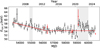 |
Fig. 1. Long-term evolution of the centroid energy of the harmonic cyclotron line in Vela X-1 as observed with Swift/BAT. The gray shaded regions indicate epochs of apparent Ecyc, H humps and the red points represent the time-averaged results from NuSTAR observations in Section 3.2.1. |
 (2)
(2)
Here E0 is the reference energy at fixed epoch t0 = 53371 (MJD), a is the linear slope describing the decreasing trend, and tcrit is the break time after which Ecyc, H remains constant. The resulting tcrit is MJD 56293 ± 264. The decrease rate of Ecyc, H is −0.584 ± 0.073 keV yr−1. After the break, the Ecyc, H remains constant at 54.60 ± 0.83 keV. Over the evolution, two abrupt humps are apparent, occurring around MJD 55000, and between MJD 59000 and MJD 60000.
3.2. NuSTAR result
3.2.1. The average spectra result
For the NuSTAR observations, the Fermi–Dirac cutoff model (FDcut; Tanaka 1986) provides a good fit to the continuum and was also adopted in previous studies (Fuerst et al. 2014; La Parola et al. 2016; Diez et al. 2022). The FDcut model, characterized by the photon index Γ, cutoff energy Ecut, and folding energy Efold, takes the form:
 (3)
(3)
The two CRSFs are well described with two Gaussian absorption components (gabs). In all the spectra, we detect with high significance the fundamental at ∼25 keV and the second harmonic at ∼52–55 keV. We constrained the width of the fundamental line to be half that of the harmonic line, σcyc, F = 0.5 × σcyc, H, following the approach adopted by Fuerst et al. (2014) and Diez et al. (2022). This assumption is motivated by the physical interpretation that harmonic lines originate from resonant scattering between the ground Landau level and higher excited levels (see Equation (1)). Consequently, the energies of the harmonic lines are expected to be twice that of the fundamental line, and their width scale accordingly. We adopted the tbabs absorption model, and set the abundances to wilm (Wilms et al. 2000). A single-absorption model cannot accurately describe the spectrum at lower energies because of the contribution of the absorption from the stellar wind. Therefore, we added a partial covering model pcfabs to take into account the wind structure (Fuerst et al. 2014; Diez et al. 2022). The interstellar absorption component (NH1) was fixed at 0.371 × 1022 cm−2, as determined from NASA’s HEASARC NH tool4. As NuSTAR does not provide coverage below 3 keV, it is not well suited to constraining low absorption values. In contrast, the absorption due to the stellar wind (NH2) was left as a free parameter. A Gaussian emission line centered around ∼6.4 keV was added to account for iron fluorescence. In addition, a broad Gaussian component around ∼10 keV was included, as this feature is essential for an adequate spectral fit. Similar features have been reported in previous studies of Vela X-1 (Fuerst et al. 2014; Diez et al. 2022), and in other sources, where they typically appear near the spectral cutoff energy (Nespoli et al. 2012; DeCesar et al. 2013; Nabizadeh et al. 2021). In the case of Vela X-1, this feature has not been interpreted as a CRSF, although its physical origin remains uncertain. To enable joint fitting of the two instruments, a cross-normalization constant was applied. Throughout the analysis, the cflux convolution model was used to derive all unabsorbed flux values.
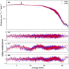 |
Fig. 2. (a) Spectrum and best-fit model for ObsID 91002349002 in energy range 3–70 keV using the model const×tbabs×pcfabs(gauss+gauss+gabs×gabs×fdcut). The FPMA data is in red and the FPMB data in blue. The best-fit model is shown in black. (b) Residuals for the best-fit model. (c) Residuals after fitting without the feature around 10 keV. (d) Residuals after fitting without the CRSFs. |
Best-fit parameters of the phase-averaged spectrum for ObsID 91002349002 using the model const×tbabs×pcfabs(gauss+gauss+gabs×gabs×fdcut) in the 3–70 keV energy band.
We present the results of ObsID 91002349002 as a representative example; this dataset has not been analyzed in previous studies. Figure 2 shows the broadband spectrum. Panel (c) presents the residuals when the ∼10 keV component is excluded from the model, and Panel (d) presents the residuals when the two CRSFs are excluded. Table 2 summarizes the spectral parameters obtained from the best-fit model for this observation. The model yielded a χ2 value of 555.27 for 448 degrees of freedom. The best-fit cyclotron line energies were  keV and
  keV. This model was subsequently applied to fit the average spectra of all NuSTAR observations. The resulting parameters are available in electronic form at the CDS. Figure 3 shows the best-fit spectral parameters, including the energy and strength of the fundamental line; the energy, width, and strength of the harmonic line; and the continuum parameters, as functions of the intrinsic source luminosity (3–70 keV) assuming a distance of 1.9 kpc. Since the measured cyclotron line energies can be affected by the continuum shape and the line widths, we also constructed corner plot of the distribution for all the parameters (see Figure A.1 in the Appendix).
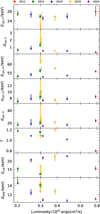 |
Fig. 3. Flux-resolved spectral parameters derived from nine NuSTAR observations in the 3–70 keV energy range, shown as a function of intrinsic source luminosity. From top to bottom: Energy of the fundamental line, energy of the harmonic line, width of the harmonic line, strength of the harmonic line, photon index, cutoff energy, and folding energy. |
The luminosity range derived from the time-averaged spectral analysis is approximately (0.2 − 0.8)×1037 erg s−1. We observed a sudden drop in Ecut at around 0.3 × 1037 erg s−1. For the three corresponding observations, we fixed Ecut at 20 keV. This adjustment has no significant impact on the parameters of either the harmonic or the fundamental cyclotron lines. The observed drop is likely due to relatively low statistics in these spectra. No clear trend is observed in the evolution of Ecyc, F with luminosity; the values range from a minimum of  keV to a maximum of
  keV. Similarly, no obvious correlation between Ecyc, H and luminosity can be established based on the nine averaged measurements. The three 2020 observations show relatively high values of Ecyc, H, reaching
  keV (ObsID 90602328002),
  keV (ObsID 90602328004), and
  keV (ObsID 90602328006), consistent with the increase in the line energy observed with the Swift/BAT monitoring since 2020. To more accurately trace the evolution of the line energy, we employed a pulse-to-pulse analysis technique.
3.2.2. The pulse-to-pulse analysis
Following the method introduced by Klochkov et al. (2011), we generated pulse amplitude-resolved spectra based on the pulse-to-pulse technique. This approach was applied to explore the luminosity dependence of the CRSF energy in Cep X–4 and V 0332+53 using NuSTAR data (Vybornov et al. 2017, 2018), and in 1A 0535+262 with Insight-HXMT data (Shui et al. 2024). The pulse-to-pulse technique is based on the fact that most accreting pulsars exhibit strong pulse-to-pulse variations in amplitude that are driven by short-term fluctuations in the accretion rate. By selecting individual pulses with similar amplitudes and grouping them to generate spectra, this method extends the accessible luminosity range and improves statistics. Therefore, it enables a more detailed investigation of the luminosity dependence of the CRSF energy.
The pulse amplitude is defined as the total number of counts summed over a single pulse. Due to limited photon statistics, extracting meaningful spectra from individual pulses is not feasible. Therefore, pulses with similar amplitudes were grouped together. We explored the distribution of pulse amplitudes and divided the entire range of amplitudes into several bins, thus ensuring approximately equal statistics within each bin. The number of bins was primarily determined by the available counting statistics for the energy spectra, which needed to be sufficient to constrain the cyclotron line energy during spectral fitting. For each bin a list of good time intervals (GTIs) was generated to select pulses within the corresponding amplitude range. Using these GTIs, we extracted the broadband spectra for each amplitude bin.
Using the pulse-to-pulse method, we divided ObsIDs 10002007001, 30002007003, 90402339002, 30501003002, and 91002349002 into 4, 4, 4, 4, and 3 amplitude bins, respectively. The distributions of counts per individual pulse are shown in Figure 4. The distributions reveal that pulse amplitudes within a single observation cover a dynamic range of several times, indicating a strong intrinsic pulse-to-pulse variability of the source. For ObsIDs 30002007002, 90602328002, 90602328004, and 90602328006, due to limited exposure time, we retained only the time-averaged spectral results. For the spectral analysis, we employed the same model as used in the time-averaged analysis: const×tbabs×pcfabs(gauss+gauss+gabs×gabs×fdcut). Given the shorter exposure time per pulse-to-pulse spectrum, we had to fix some parameters to their respective time-averaged values to achieve a good fit. We fixed the width of the iron line, σKα; the energy and the width of the 10 keV line, E10 keV and σ10 keV; and the width of the two CRSFs, σcyc, F and σcyc, H, to their respective time-averaged values. We initially attempted to leave σcyc, H and Ecut free. However, this approach resulted in poor constraints on Ecut. The continuum parameter Ecut was therefore fixed because of its degeneracy with the fundamental line energy Ecyc, F. With the adopted strategy of fixing the above parameters, we obtained very good fits for all spectra. The corresponding best-fit parameters are provided in the tables available at the CDS.
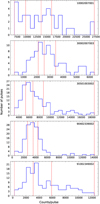 |
Fig. 4. Distributions of counts per individual pulse (i.e. of pulse amplitudes). The red dashed lines indicate the boundaries of the amplitude bins used for extracting pulse-to-pulse spectra. In each distribution, the total number of counts is evenly distributed among the bins. |
Figure 5 presents the spectral results obtained from the pulse-to-pulse analysis. The plot also includes the time-averaged results for the short-exposure observations 30002007002, 90602328002, 90602328004, and 90602328006. Our analysis extends the explored luminosity range to (0.13 − 1.21)×1037 erg s−1 and successfully disentangles the intrinsic long-term evolution of Ecyc from its luminosity dependence.
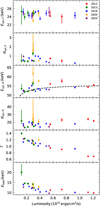 |
Fig. 5. Flux-resolved spectral parameters derived from the pulse-to-pulse analysis in the 3–70 keV energy range. Different colors represent different observation years, and distinct marker styles indicate observation IDs; time-averaged results for the short-exposure observations (30002007002, 90602328002, 90602328004, and 90602328006) are also shown. The dashed line in the second panel is the theoretical prediction for E* = 28.097 ± 0.052 keV (see Equation (4)). |
The fundamental line energy, Ecyc, F, exhibits no significant variation with time or luminosity, remaining stable at approximately 25 keV. At higher luminosities (LX ≳ 1037 erg s−1), the spectra can be well fit without requiring an additional component for the fundamental line. Therefore, we do not include these two data points in the plot, as they are not meaningful when the corresponding spectral component is not necessary for the fit. To improve the statistics, we split this observation into two bins, with only one data point in the high-luminosity bin. The fit remains acceptable without the fundamental line. When included, we derived a 3σ upper limit on its strength of ∼0.8, suggesting that the line may be present but undetectable due to limited sensitivity.
For the energy of harmonic line, Ecyc, H, excluding the 2020 observations, the data appear fairly stable, with slightly lower values at lower luminosities. Moreover, at comparable luminosity levels, there is no time dependence of the Ecyc, H across different epochs, suggesting that the long-term decay of Ecyc, H likely ceased after 2012. Additionally, the photon index exhibits a negative correlation with luminosity, indicating a hardening of the continuum spectrum at higher flux levels.
4. Discussion
In this work, we investigate the dependence of the fundamental cyclotron line energy (Ecyc, F) and the harmonic line energy (Ecyc, H) on both time and X-ray luminosity (LX). By performing a time-averaged analysis of archival Swift/BAT monitoring data, we investigated the long-term evolution of Ecyc, H over 20 years. Using observations from NuSTAR we performed the pulse-to-pulse analysis to reveal the comprehensive scenario of the Ecyc–LX relation covering a luminosity range of 0.13 × 1037 erg s−1 to 1.21 × 1037 erg s−1.
4.1. Changes in Ecyc with time
To date, only two sources, Her X-1 and Vela X-1, have shown clear long-term variability in Ecyc over timescales of tens of years (Staubert et al. 2020; La Parola et al. 2016; Ji et al. 2019). In Her X-1 the long-term decay of Ecyc ended around 2012, stabilizing at approximately 37 keV, with a decline rate of ∼0.26 keV yr−1 between 1996 and 2012 (Staubert et al. 2020). For Vela X-1 our analysis confirms the previously reported decrease in the energy of the first cyclotron harmonic (La Parola et al. 2016; Ji et al. 2019), which now appears to remain constant. The decrease rate is ∼0.36 keV yr−1 and ∼0.51 keV yr−1 stated by La Parola et al. (2016) and Ji et al. (2019), similar to our result ∼0.58 keV yr−1 based on BAT observations.
The long-term decay of Ecyc, H in Vela X-1 is likely a local effect at the magnetic polar cap, rather than a change in the global dipole field. Similar scenarios have been proposed for Her X-1 (Staubert et al. 2014, 2016, 2020). They suggested that the decay could be connected to a geometric displacement of the emission region in the dipole field or it could be related to the accreted matter that accumulates into a magnetically supported mound and causes a change in the magnetic field configuration at the polar cap. The end of the decay could be explained by the mound reaching its maximum stable size beyond which further accumulation no longer significantly affects the field structure.
In addition, we observed a sudden increase in the harmonic cyclotron line energy, reaching ∼62 keV in 2020, with NuSTAR observations, followed by a decrease back to ∼52 keV in 2024 at comparable luminosity levels of ∼0.3 × 1036 erg s−1. Such a dramatic evolution in the cyclotron line energy is unusual. This result is supported by Swift/BAT monitoring, which shows a significant increase in Ecyc, H between 2020 and 2023 (MJD 59000–60000). A similar hump around MJD 55000 was also detected in the Swift/BAT data and was reported by Ji et al. (2019). A comparable phenomenon was observed in Her X-1, where the line energy remained constant prior to 1991 and then increased to ∼41 keV between 1990 and 1995 (Gruber et al. 1999; dal Fiume et al. 1998), followed by a more gradual, linear decay. This process may be cyclic (Staubert et al. 2017).
We present here a possible explanation for the sudden increase. Matter accumulation at the magnetic poles increases the overpressure until a critical threshold is reached. This triggers interchange instabilities (e.g., ballooning instabilities Litwin et al. 2001) near the column boundary, causing localized magnetic field deformation and mass leakage. As a result, Ecyc, H increases because of partial column collapse, and a reduction in height. The fact that only Ecyc, H exhibits this strong variability, while the Ecyc, F remains nearly constant, may suggest that the harmonic line is more sensitive to changes in the height of the emission region.
It is worth noting that previous studies have shown that sudden changes in cyclotron line energy generally occur during the declining phase of long-term evolution. In contrast, this work is the first to reveal that such abrupt shifts can also arise when the cyclotron line has entered a relatively stable, long-term plateau. This finding suggests that even when the polar-cap accretion structure appears to have reached a steady state, localized regions may still experience dynamic or structural changes. At present, no comprehensive theoretical framework can fully explain this behavior, but extensive future observations of Vela X-1 and other source (e.g. Her X-1, Cen X-3, 4U 1538-522) could provide critical constraints for refining models of polar-cap dynamics and magnetic-field evolution.
4.2. Changes in Ecyc with luminosity
The variation in Ecyc with luminosity has long been a key focus in the study of accreting X-ray pulsars because it directly reflects the strength of the local magnetic field. Previous observations suggest that cyclotron lines exhibit two distinct evolutionary trends depending on luminosity. A positive dependence of Ecyc on LX was observed in low- to moderate-luminosity sources, such as Her X-1 (Staubert et al. 2007, 2014, 2016, 2017, 2020), Vela X-1 (Fuerst et al. 2014; La Parola et al. 2016; Diez et al. 2022), and Cep X-4 (Vybornov et al. 2017). A negative dependence of Ecyc on LX was observed in relatively high-luminosity sources, such as V 0332+53 (Tsygankov et al. 2006; Cusumano et al. 2016; Doroshenko et al. 2017; Vybornov et al. 2018) and 1A 0535+262 (Kong et al. 2021). The luminosity at which these different evolutionary behaviors of Ecyc occur is often referred to as the critical luminosity (Lcrit) of the source, typically a few times 1037 erg s−1. The Lcrit separates the accretion regimes into sub-critical and super-critical states. In general, sub-critical accretion is associated with a positive Ecyc–LX correlation, while super-critical accretion corresponds to a negative correlation (Becker et al. 2012; Mushtukov et al. 2015a). The contrasting Ecyc–LX behaviors at sub-critical and super-critical luminosities can be interpreted within different theoretical models. An interpretation for the observed Ecyc–LX correlation relies on the relationship between the Ecyc and the height of the emission region above the NS surface (Becker et al. 2012). In low- to moderate-luminosity sources, including Vela X-1, the accreting material is primarily decelerated via Coulomb braking. As the accretion rate increases, the emission region is pushed closer to the NS surface, where the magnetic field is stronger, leading to an increase in Ecyc. Mushtukov et al. (2015b) proposed that the positive correlation observed in sub-critical sources arises from Doppler shifts in the infalling plasma. In this model, CRSFs are formed as radiation from the polar-cap hotspot travels upward through the accretion column and interacts with the plasma at resonant energies. As luminosity increases, radiation pressure slows the plasma, thus reducing the Doppler redshift and causing the observed line energy to rise.
In our study we first focused on the harmonic cyclotron line energy, Ecyc, H. Using two NuSTAR observations from 2012 and 2013, Fuerst et al. (2014) reported a positive correlation between Ecyc, H and luminosity. However, Diez et al. (2022), based on two NuSTAR observations from 2019, were unable to confirm this correlation. According to our results, the data remain relatively stable, exhibiting modestly reduced values at lower luminosities. Theoretical predictions for the Ecyc–LX relationship can be derived from Equations (51) and (58) of Becker et al. (2012):
![Mathematical equation: $$ \begin{aligned} \begin{aligned} E_{\rm theo} =&\left[1 + 0.6 \left(\frac{R_*}{10\,\mathrm{km}}\right)^{-\frac{13}{14}}\left(\frac{\Lambda }{0.1}\right)^{-1}\left(\frac{\tau _*}{20}\right) \times \left(\frac{M_*}{1.4\,M_{\odot }}\right)^{\frac{19}{14}}\right.\\&\left.\left(\frac{E_*}{1\,\mathrm{keV}}\right)^{-\frac{4}{7}}\left(\frac{L_x}{10^{37}\,\mathrm{{erg\,s}}^{-1}}\right)^{-\frac{5}{7}}\right]^{-3}\times E_*. \end{aligned} \end{aligned} $$](/articles/aa/full_html/2026/02/aa56470-25/aa56470-25-eq31.gif) (4)
(4)
Here τ* is the Thomson optical depth, around 20 for typical HMXB parameters (Becker et al. 2012), and E* is the energy of the fundamental cyclotron line at the NS surface. We adopt the values Λ = 1, R* = 10 km and M* = 1.8 M⊙. Fitting the data using Equation (4) and excluding the anomalously high values from 2020 yields E* = 28.097 ± 0.052 keV, assuming a harmonic ratio of 2. The Pearson correlation coefficient is 0.462, with a p-value of 0.0405.
However, the fundamental line shows a different behavior as a function of luminosity. A possible anti-correlation up to 7 × 1036 erg s−1 was reported by Fuerst et al. (2014), beyond which the correlation seems to flatten. This result is obtained from the fitting of data from each orbit, with relatively short exposure times, which leads to large error bars. In our pulse-to-pulse analysis, we considered both the spectra with similar pulse amplitudes and those with longer exposures. As a result, our findings provide better constraints on the fundamental cyclotron line and confirm that its energy shows a flat evolutionary trend with luminosity. The lack of a clear luminosity dependence in the fundamental CRSF energy can be explained by the photon spawning effect (Schönherr et al. 2007). In this scenario, resonant scattering events produce additional low-energy photons that preferentially populate the energy range of the fundamental line, effectively filling in the absorption feature and diminishing its depth. As a result, the fundamental line becomes less sensitive to luminosity. Furthermore, based on Harding & Daugherty (1991), the cross section of CRSF at the fundamental and the harmonic is different, which is related to the angle between the photon momentum and the magnetic field. In the subcritical regime, photons can escape from the top of the accretion column along the magnetic field lines (called pencil-beam geometry), where the cross section of the harmonic line is much lower than that of the fundamental, making it intrinsically weaker. However, when the infalling material reaches relativistic speeds, the resulting beaming effect can increase the effective viewing angle and enhance the cross section of the harmonic line. Such conditions may arise near the shock region of the accretion column, leading to a locally stronger harmonic feature (see discussion in Kong et al. 2022).
To further investigate the accretion regime of Vela X-1, we calculated the Lcrit under different theoretical models. The expression for the Lcrit as a function of the magnetic field strength at the neutron star (NS) surface, following Becker et al. (2012), is given by:
 (5)
(5)
where R* is the radius of the NS, M* is the mass of the NS, B* is the magnetic field strength at the NS surface, Λ is a constant that depends on the accretion flow geometry, and w is a parameter describing the spectral shape inside the column. We adopt R* = 10 km and M* = 1.8 M⊙ (Rawls et al. 2011), and assume w = 1, corresponding to a Bremsstrahlung-dominated emission spectrum inside the column. Accretion flow geometry is a source of principal uncertainties. If we take Λ = 1, appropriate for spherical or wind-fed accretion, and combine Equation (5) with Equation (1), assuming a surface fundamental cyclotron line energy of Ecyc, F = 25 keV, we obtain Lcrit ∼ 0.17 × 1037 erg s−1. If we adopt Λ = 0.1, which corresponds to disc accretion, yields Lcrit ∼ 4.31 × 1037 erg s−1. These two scenarios represent limiting cases. In reality, the accretion flow may involve a combination of both modes, suggesting that the actual Lcrit lies between these two limits.
Mushtukov et al. (2015a) provided a numerical solution by calculating the luminosity for two scenarios: one with purely extraordinary polarization and another with an equal mix of ordinary and extraordinary polarization. The real critical luminosity value is expected to fall between the two cases. In their prediction, assuming Ecyc = 25 keV, the estimated Lcrit for Vela X-1 is in the range of ∼0.3 − 1.0 × 1037 erg s−1 (as shown in Fig. 7 of that study).
We observe a clear spectral hardening with increasing luminosity. In many accreting pulsars, the photon index Γ exhibits a luminosity dependence similar to that of the Ecyc: it decreases with increasing luminosity in high-luminosity sources (i.e., the spectrum softens), and increases with luminosity in low- to moderate-luminosity sources (i.e., the spectrum hardens) (Klochkov et al. 2011; Reig & Nespoli 2013). In the case of Vela X-1, this behavior can be interpreted as a result of the emission region moving closer to the neutron star surface at higher luminosities. As the sinking region becomes more compact, the optical depth increases, leading to enhanced Comptonization and the production of harder photons, thereby yielding a harder spectrum (Becker et al. 2012; Reig & Nespoli 2013). According to the model proposed by Postnov et al. (2015), at low luminosities the emerging X-ray spectrum is produced by ordinary photons in a magnetized optically thin slab-like atmosphere near the polar cap. As the accretion rate increases, the Comptonization rises, thus leading to a harder X-ray continuum.
5. Conclusions
We conducted a detailed study of the long-term evolution and the luminosity dependence of the cyclotron line energy in Vela X-1, based on archival Swift/BAT monitoring and nine NuSTAR observations from 2012 to 2024.
This work presented the first confirmation that the long-term decay of the harmonic line energy in Vela X-1 has ended. Moreover, we report the first detection of a renewed increase in Ecyc, H between 2020 and 2023. Such dramatic variability, which occurred after the line energy had settled into a relatively stable plateau, is unusual and likely reflects sudden magnetic or structural changes in the accretion environment. Continued long-term monitoring of Vela X-1 and other sources will be essential to determine whether this behavior is part of a broader cyclic phenomenon.
Using pulse-to-pulse analysis, we find that the fundamental line energy remains stable over both time and luminosity, showing no significant evolution. The harmonic line energy is found to be slightly lower at low luminosities and to flatten at higher luminosities.
Data availability
The tables related to the Swift/BAT spectral parameters, the NuSTAR averaged spectral parameters, and the NuSTAR pulse-to-pulse spectral parameters for individual observations are available at the CDS via https://cdsarc.cds.unistra.fr/viz-bin/cat/J/A+A/706/A175
Acknowledgments
This work made use of data from the NuSTAR mission, a project led by the California Institute of Technology, and also benefited from the long-term support of the Burst Alert Telescope on board the Neil Gehrels Swift observatory. Y.J. Du would like to thank the support from China Scholarship Council (CSC 202108080247). P. J. Wang is grateful for the financial support provided by the Sino-German (CSC-DAAD) Postdoc Scholarship Program (57678375). L. Ji is supported by the National Natural Science Foundation of China under grant No. 12173103. LD acknowledges funding from the Deutsche Forschungsgemeinschaft (DFG, German Research Foundation) – Projektnummer 549824807.
References
- Barthelmy, S. D., Barbier, L. M., Cummings, J. R., et al. 2005, Space Sci. Rev., 120, 143 [Google Scholar]
- Becker, P. A., Klochkov, D., Schönherr, G., et al. 2012, A&A, 544, A123 [NASA ADS] [CrossRef] [EDP Sciences] [Google Scholar]
- Chodil, G., Mark, H., Rodrigues, R., Seward, F. D., & Swift, C. D. 1967, ApJ, 150, 57 [NASA ADS] [CrossRef] [Google Scholar]
- Cusumano, G., La Parola, V., D’Aì, A., et al. 2016, MNRAS, 460, L99 [NASA ADS] [CrossRef] [Google Scholar]
- dal Fiume, D., Orlandini, M., Cusumano, G., et al. 1998, A&A, 329, L41 [Google Scholar]
- DeCesar, M. E., Boyd, P. T., Pottschmidt, K., et al. 2013, ApJ, 762, 61 [NASA ADS] [CrossRef] [Google Scholar]
- Diez, C. M., Grinberg, V., Fürst, F., et al. 2022, A&A, 660, A19 [NASA ADS] [CrossRef] [EDP Sciences] [Google Scholar]
- Doroshenko, V., Tsygankov, S. S., Mushtukov, A. A., et al. 2017, MNRAS, 466, 2143 [NASA ADS] [CrossRef] [Google Scholar]
- Fuerst, F., Pottschmidt, K., Wilms, J., et al. 2014, American Astronomical Society Meeting Abstracts, 223, 438.20 [Google Scholar]
- Fürst, F., Kreykenbohm, I., Pottschmidt, K., et al. 2010, A&A, 519, A37 [CrossRef] [EDP Sciences] [Google Scholar]
- Gehrels, N., Chincarini, G., Giommi, P., et al. 2004, ApJ, 611, 1005 [Google Scholar]
- Gruber, D. E., Heindl, W. A., Rothschild, R. E., et al. 1999, in Highlights in X-ray Astronomy, eds. B. Aschenbach, & M. J. Freyberg, 272, 33 [NASA ADS] [Google Scholar]
- Harding, A. K., & Daugherty, J. K. 1991, ApJ, 374, 687 [NASA ADS] [CrossRef] [Google Scholar]
- Harrison, F. A., Craig, W. W., Christensen, F. E., et al. 2013, ApJ, 770, 103 [Google Scholar]
- Hiltner, W. A., Werner, J., & Osmer, P. 1972, ApJ, 175, L19 [Google Scholar]
- Ji, L., Staubert, R., Ducci, L., et al. 2019, MNRAS, 484, 3797 [Google Scholar]
- Kendziorra, E., Mony, B., Kretschmar, P., et al. 1992, in Frontiers Science Series, eds. Y. Tanaka, & K. Koyama, 51 [Google Scholar]
- Klochkov, D., Staubert, R., Santangelo, A., Rothschild, R. E., & Ferrigno, C. 2011, A&A, 532, A126 [NASA ADS] [CrossRef] [EDP Sciences] [Google Scholar]
- Klochkov, D., Staubert, R., Postnov, K., et al. 2015, A&A, 578, A88 [NASA ADS] [CrossRef] [EDP Sciences] [Google Scholar]
- Kong, L. D., Zhang, S., Ji, L., et al. 2021, ApJ, 917, L38 [NASA ADS] [CrossRef] [Google Scholar]
- Kong, L.-D., Zhang, S., Ji, L., et al. 2022, ApJ, 932, 106 [Google Scholar]
- Kretschmar, P., Pan, H. C., Kendziorra, E., et al. 1997, A&A, 325, 623 [NASA ADS] [Google Scholar]
- Kretschmar, P., El Mellah, I., Martínez-Núñez, S., et al. 2021, A&A, 652, A95 [NASA ADS] [CrossRef] [EDP Sciences] [Google Scholar]
- Kreykenbohm, I., Coburn, W., Wilms, J., et al. 2002, A&A, 395, 129 [NASA ADS] [CrossRef] [EDP Sciences] [Google Scholar]
- La Parola, V., Cusumano, G., Segreto, A., & D’Aì, A. 2016, MNRAS, 463, 185 [NASA ADS] [CrossRef] [Google Scholar]
- Leahy, D. A. 1987, A&A, 180, 275 [NASA ADS] [Google Scholar]
- Litwin, C., Brown, E. F., & Rosner, R. 2001, ApJ, 553, 788 [Google Scholar]
- Maitra, C., & Paul, B. 2013, ApJ, 763, 79 [NASA ADS] [CrossRef] [Google Scholar]
- Mushtukov, A. A., Suleimanov, V. F., Tsygankov, S. S., & Poutanen, J. 2015a, MNRAS, 447, 1847 [NASA ADS] [CrossRef] [Google Scholar]
- Mushtukov, A. A., Tsygankov, S. S., Serber, A. V., Suleimanov, V. F., & Poutanen, J. 2015b, MNRAS, 454, 2714 [Google Scholar]
- Nabizadeh, A., Tsygankov, S. S., Ji, L., et al. 2021, A&A, 652, A89 [NASA ADS] [CrossRef] [EDP Sciences] [Google Scholar]
- Nespoli, E., Reig, P., & Zezas, A. 2012, A&A, 547, A103 [NASA ADS] [CrossRef] [EDP Sciences] [Google Scholar]
- Odaka, H., Khangulyan, D., Tanaka, Y. T., et al. 2013, ApJ, 767, 70 [Google Scholar]
- Postnov, K. A., Gornostaev, M. I., Klochkov, D., et al. 2015, MNRAS, 452, 1601 [Google Scholar]
- Rawls, M. L., Orosz, J. A., McClintock, J. E., et al. 2011, ApJ, 730, 25 [NASA ADS] [CrossRef] [Google Scholar]
- Reig, P., & Nespoli, E. 2013, A&A, 551, A1 [NASA ADS] [CrossRef] [EDP Sciences] [Google Scholar]
- Sadakane, K., Hirata, R., Jugaku, J., et al. 1985, ApJ, 288, 284 [Google Scholar]
- Schanne, S., Götz, D., Gérard, L., et al. 2007, in The Obscured Universe. Proceedings of the VI Integral Workshop, ESA SP, 622, 479 [Google Scholar]
- Schönherr, G., Wilms, J., Kretschmar, P., et al. 2007, A&A, 472, 353 [NASA ADS] [CrossRef] [EDP Sciences] [Google Scholar]
- Shui, Q. C., Zhang, S., Wang, P. J., et al. 2024, MNRAS, 528, 7320 [NASA ADS] [CrossRef] [Google Scholar]
- Staubert, R., Shakura, N. I., Postnov, K., et al. 2007, A&A, 465, L25 [NASA ADS] [CrossRef] [EDP Sciences] [Google Scholar]
- Staubert, R., Klochkov, D., Wilms, J., et al. 2014, A&A, 572, A119 [NASA ADS] [CrossRef] [EDP Sciences] [Google Scholar]
- Staubert, R., Klochkov, D., Vybornov, V., Wilms, J., & Harrison, F. A. 2016, A&A, 590, A91 [NASA ADS] [CrossRef] [EDP Sciences] [Google Scholar]
- Staubert, R., Klochkov, D., Fürst, F., et al. 2017, A&A, 606, L13 [NASA ADS] [CrossRef] [EDP Sciences] [Google Scholar]
- Staubert, R., Trümper, J., Kendziorra, E., et al. 2019, A&A, 622, A61 [NASA ADS] [CrossRef] [EDP Sciences] [Google Scholar]
- Staubert, R., Ducci, L., Ji, L., et al. 2020, A&A, 642, A196 [NASA ADS] [CrossRef] [EDP Sciences] [Google Scholar]
- Tanaka, Y. 1986, in IAU Colloquium 89: Radiation Hydrodynamics in Stars and Compact Objects, eds. D. Mihalas, & K.-H. A. Winkler, 255, 198 [Google Scholar]
- Tsygankov, S. S., Lutovinov, A. A., Churazov, E. M., & Sunyaev, R. A. 2006, MNRAS, 371, 19 [NASA ADS] [CrossRef] [Google Scholar]
- Vybornov, V., Klochkov, D., Gornostaev, M., et al. 2017, A&A, 601, A126 [NASA ADS] [CrossRef] [EDP Sciences] [Google Scholar]
- Vybornov, V., Doroshenko, V., Staubert, R., & Santangelo, A. 2018, A&A, 610, A88 [NASA ADS] [CrossRef] [EDP Sciences] [Google Scholar]
- Wilms, J., Allen, A., & McCray, R. 2000, ApJ, 542, 914 [Google Scholar]
Appendix A: Additional figure
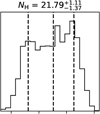 |
Fig. A.1. Corner plot of the posterior distributions of all model parameters for ObsID 91002349002. |
All Tables
Best-fit parameters of the phase-averaged spectrum for ObsID 91002349002 using the model const×tbabs×pcfabs(gauss+gauss+gabs×gabs×fdcut) in the 3–70 keV energy band.
All Figures
|
Fig. 1. Long-term evolution of the centroid energy of the harmonic cyclotron line in Vela X-1 as observed with Swift/BAT. The gray shaded regions indicate epochs of apparent Ecyc, H humps and the red points represent the time-averaged results from NuSTAR observations in Section 3.2.1. |
| In the text | |
|
Fig. 2. (a) Spectrum and best-fit model for ObsID 91002349002 in energy range 3–70 keV using the model const×tbabs×pcfabs(gauss+gauss+gabs×gabs×fdcut). The FPMA data is in red and the FPMB data in blue. The best-fit model is shown in black. (b) Residuals for the best-fit model. (c) Residuals after fitting without the feature around 10 keV. (d) Residuals after fitting without the CRSFs. |
| In the text | |
|
Fig. 3. Flux-resolved spectral parameters derived from nine NuSTAR observations in the 3–70 keV energy range, shown as a function of intrinsic source luminosity. From top to bottom: Energy of the fundamental line, energy of the harmonic line, width of the harmonic line, strength of the harmonic line, photon index, cutoff energy, and folding energy. |
| In the text | |
|
Fig. 4. Distributions of counts per individual pulse (i.e. of pulse amplitudes). The red dashed lines indicate the boundaries of the amplitude bins used for extracting pulse-to-pulse spectra. In each distribution, the total number of counts is evenly distributed among the bins. |
| In the text | |
|
Fig. 5. Flux-resolved spectral parameters derived from the pulse-to-pulse analysis in the 3–70 keV energy range. Different colors represent different observation years, and distinct marker styles indicate observation IDs; time-averaged results for the short-exposure observations (30002007002, 90602328002, 90602328004, and 90602328006) are also shown. The dashed line in the second panel is the theoretical prediction for E* = 28.097 ± 0.052 keV (see Equation (4)). |
| In the text | |
|
Fig. A.1. Corner plot of the posterior distributions of all model parameters for ObsID 91002349002. |
| In the text | |
Current usage metrics show cumulative count of Article Views (full-text article views including HTML views, PDF and ePub downloads, according to the available data) and Abstracts Views on Vision4Press platform.
Data correspond to usage on the plateform after 2015. The current usage metrics is available 48-96 hours after online publication and is updated daily on week days.
Initial download of the metrics may take a while.