| Issue |
A&A
Volume 706, February 2026
|
|
|---|---|---|
| Article Number | A158 | |
| Number of page(s) | 9 | |
| Section | Stellar structure and evolution | |
| DOI | https://doi.org/10.1051/0004-6361/202556508 | |
| Published online | 06 February 2026 | |
Multiple short-term cycles in Kepler star KIC 6876668
1
Georg-August-Universität, Institut für Astrophysik Friedrich-Hund-Platz 1 37077 Göttingen, Germany
2
E. Kharadze Georgian National Astrophysical Observatory Mount Kanobili, Georgia
3
School of Natural Sciences and Medicine, Ilia State University Cholokashvili Ave. 3/5 Tbilisi, Georgia
4
Institute of Physics, IGAM, University of Graz Universitätsplatz 5 8010 Graz, Austria
5
INAF-Osservatorio Astrofisico di Catania, Via S. Sofia 78 95123 Catania, Italy
6
Departament de Física & Institut d’Aplicacions Computacionals de Codi Comunitari (IAC3), Universitat de les Illes Balears 07122 Palma de Mallorca, Spain
★ Corresponding author: This email address is being protected from spambots. You need JavaScript enabled to view it.
Received:
19
July
2025
Accepted:
21
November
2025
Abstract
Context. Solar and stellar magnetic activity may have similar properties, which can be used to understand the stellar magnetic evolution.
Aims. This paper examines the multiple short-term cycles in the total irradiance of the Sun and in the light curve of a Kepler star, KIC 6876668.
Methods. We study the light curve variations of KIC 6876668, which exhibits a rotation period of 5−6 d. In order to detect cyclic patterns across rotational and Rieger timescales, we used wavelet and Lomb-Scargle (LS) methodologies.
Results. We found that the light curve of the star exhibits periodicities at ∼47, 59 and 72 d, which are fully consistent with the Rieger period range. Through LS and wavelet analysis, we also found variations in the total irradiance of the Sun as a star in cycle 23 of ∼185, 240, and 380 d. The ratios of stellar and solar cyclic periods over their rotation periods revealed striking similarities of ∼8, ∼10, and 12−15. The observed cycles are interpreted as the spherical harmonics of magnetic Rossby waves in dynamo layers of the star and the Sun. The corresponding magnetic field strengths are estimated as 40 kG and 10 kG in the stellar and solar interiors, respectively. The relationship observed between the Rieger cycle and the rotation period of a young star suggests that the processes in its inner layers driving stellar cycles resemble those found in the Sun.
Conclusions. These results provide an insight into the internal magnetic processes in a Sun-like star, KIC 6876668, where a short cycle and a strong magnetic field indicate stronger activity. Sun-like stars as well as other stars may show similar variations in magnetic activity to the Sun. Therefore, the cycles can be used to extract plasma parameters in their interior. Our analysis shows that the ratio of the rotation angular frequency and the estimated magnetic field strength might stay constant (Ω/B = constant) throughout stellar evolution.
Key words: stars: activity / stars: evolution / stars: magnetic field / stars: solar-type / starspots
© The Authors 2026
 Open Access article, published by EDP Sciences, under the terms of the Creative Commons Attribution License (https://creativecommons.org/licenses/by/4.0), which permits unrestricted use, distribution, and reproduction in any medium, provided the original work is properly cited.
This article is published in open access under the Subscribe to Open model. This email address is being protected from spambots. You need JavaScript enabled to view it. to support open access publication.
1. Introduction
Main-sequence stars generally follow an activity-rotation relationship in which faster-rotating stars are more active. Stellar activity is often quasi-periodic, resembling the Schwabe cycles of 11 years on the Sun, but the variation timescales are rather dispersed. The ratio of cyclic and rotational frequencies, which is generally proportional to Rossby number, has two different scales for most stars with age t > 0.1 Gyr: the stars are distributed in two parallel branches on a cyclic period-Rossby number diagram, where more active stars are more widely distributed in the lower branch and then fall to the upper branch with increasing age (Saar & Brandenburg 1999). However, after studying the chromospheric activity of 4454 cool stars, Boro Saikia et al. (2018) strongly questioned the existence of an active branch of stellar activity cycles.
On the other hand, the Schwabe cycles in solar activity are accompanied by the variations over shorter timescales. The short-term periodicity of several months, called Rieger-type cycles, was discovered almost 40 years ago in γ-ray solar flares (Rieger et al. 1984). The periodicity has been reported in many indices of solar activity such as sunspots, flares, radio flux, and total solar irradiance (Bai & Sturrock 1987; Bai & Cliver 1990; Carbonell & Ballester 1990, 1992; Oliver et al. 1998; Zaqarashvili et al. 2010; Gurgenashvili et al. 2021). It was found that the periodicity appears or disappears in different cycles and has different values for different indices (Lean & Brueckner 1989; Lean 1990). Previous studies have suggested that the Rieger cycle manifests as a relatively short periodicity, typically ranging between 150 and 250 days in the case of the Sun (Lean 1990; Oliver et al. 1998; Zaqarashvili et al. 2010; Gurgenashvili et al. 2016). It was recently shown that the Rieger periodicity correlates with solar cycle strength so that shorter periods are found in stronger cycles and in more active hemispheres (Gurgenashvili et al. 2016, 2017). The observed correlation of the Rieger period with solar cycle strength suggests its possible connection with the solar internal dynamo layer below the convection zone. This hypothesis is further supported by the detection of Rieger cycles in erupted magnetic flux (Ballester et al. 2002). Therefore, the Rieger periodicity might appear in the dynamo layer below the convection zone.
The physical mechanism of Rieger periodicity remains an open question. Various mechanisms have been proposed to explain the properties of this periodicity. Ichimoto et al. (1985) suggested that the periodicity might be linked to the timescale of the magnetic field in the solar convective zone. Bai & Sturrock (1991) introduced a ‘clock’ model with a rotation period of 25−28 d, interpreting the 155-d period as a subharmonic of the tenth fundamental period. Wolff (1992) and Sturrock et al. (2013) attempted to explain this periodicity through oscillations of non-magnetic r-modes, or Rossby waves. Lou (2000) proposed that large-scale equatorial hydrodynamic Rossby waves in the photosphere could be responsible.
Because the periodicity is observed in the magnetic flux-related activity indices (for example, it is absent in plage-index, where the magnetic field is very weak), the inclusion of magnetic field in Rossby wave model is essential. Zaqarashvili et al. (2010) showed that this periodicity can be explained by Rossby waves in the solar tachocline, where the combined action of differential rotation and a toroidal magnetic field drive instabilities. The unstable harmonics of Rossby waves can cause periodic magnetic flux surges at the surface. The dispersion relation of magnetic Rossby waves depends on the magnetic field strength, so cycle-to-cycle variations in the dynamo field naturally modulate the observed periodicity.
Then the observed periodicity might be used to sound the magnetic field in the dynamo layer using the dispersion relation of the magnetic Rossby waves (Zaqarashvili & Gurgenashvili 2018). This method may prove to be a very important tool for testing different dynamo models not only on the Sun but also on other solar-type stars (Zaqarashvili et al. 2021). Another short-to-intermediate cycle observed in the solar activity is the 1-yr oscillation, which has already been found in various indicators of solar activity, such as the sunspot number and area (Wolff 1983; Oliver et al. 1992; Gachechiladze et al. 2019), 10.7 cm radio flux, plage index (Lean & Brueckner 1989), and solar flares (Ichimoto et al. 1985; Bai 1987). However, typically, the 1 yr periodicity is not officially considered as a Rieger period. The 1 yr, 1.3 yr, and 2 yr cycles are known as mid-range periods in solar activity.
One can suggest the existence of shorter period cycles on other stars. Indeed, short period cycles in Sun-like stars have been known since Baliunas et al. (1995) discovered the 116-d cycle in τ Boo, which proved to be quite stable for 40 years (Mittag et al. 2017) and co-existed with a longer, 11.6-yr cycle. Later Mengel et al. (2016), Schmitt & Mittag (2017), and Mittag et al. (2017) confirmed the existence of 117−122-d cycles in the same star. Other F-type stars with short cycles are confirmed to be HD17051 (1.6 yr; Metcalfe et al. 2010) and HD49933 (120 d; García et al. 2010). Mittag et al. (2019) detected three additional F-type stars showing cycles shorter than one year.
Long-term ground-based observations have already established the connection between starspots, chromospheric activity, and stellar cycles (Wilson 1978; Noyes et al. 1984; Saar & Baliunas 1992). Later, space-based observatories, including Kepler (Borucki et al. 2010), CoRoT (Baglin et al. 2008), and TESS (Ricker et al. 2014), provided continuous, high-quality photometric monitoring of solar-type stars and extended these studies by discovering modulations caused by star spots and cyclic variations (Breton et al. 2024a). A fraction of Kepler’s stars are young, magnetically more active than the Sun, characterised by shorter rotation periods and stronger dynamos. Lanza et al. (2009) discovered a 29-d cycle in the G7 star CoRoT-2 accompanied by an orbiting hot Jupiter. A 48-d short cycle (Bonomo & Lanza 2012) was discovered in Kepler-17 (G2V star), which was later confirmed by Lanza et al. (2019) based on the 4-year complete observations of Kepler. The existence of short cycles has been confirmed on other Kepler stars as well (Arkhypov et al. 2015; Arkhypov & Khodachenko 2021). Gurgenashvili et al. (2022) found a Rieger cycle of 61-d on a Kepler Sun-like star with a rotation period of about 9.5 d. The obtained periodicity was used to estimate the magnetic field strength in the stellar internal dynamo layer.
The upcoming PLATO (PLAnetary Transits and Oscillations of Stars) mission of the European Space Agency (ESA) aims to detect and study exoplanets and conduct asteroseismic analyses of numerous stars. Aside from discovering planets that are smaller than two Earth radii around bright stars, PLATO will also find terrestrial planets within the habitable zones of solar-like stars, improving our understanding of exoplanetary systems (Rauer et al. 2025). The PLATO mission aims to focus on the Sun-like stars, including their rotations and activity cycles (Breton et al. 2024b). After Kepler and CoRoT missions, PLATO can give us new insights to better understand the processes in the stellar interiors. Among Sun-like stars, this information is crucial for improving gyrochronology (Barnes 2010) and dynamo theories. In this paper, we analyse the light curve of a Kepler star to find the short-term cycles that might be analogous to the solar Rieger-type cycles.
2. Data and methods
Several catalogues were created on the basis of Kepler data to find the parameters of stars including rotation period: Reinhold et al. (2013, 2024), Nielsen et al. (2013), McQuillan et al. (2014), Santos et al. (2019, 2021)1. The analysis shows that the periodograms of Kepler stars are mostly flat, showing only rotation periods and their half values. Significant effort is required to find the periods in their light curves, which are longer than the rotation period.
Kepler has two types of data: simple aperture photometry (SAP), which contains strong instrumental trends and pre-search data conditioning (PDC), in which the instrumental trends are mostly removed. As a result of the aggressive methods used to correct for instrumental trends, PDC data can sometimes be strongly affected and all variability over timescales of 20−25 days is strongly reduced or suppressed, especially when the applied correction algorithm is the multi-scale maximum a posteriori data (msMAP; Gilliland et al. 2015). While the periodic signals that persist after vigorous cleaning are probably very strong, we cannot entirely dismiss the probability that certain long-period signals were altered or eliminated during these correction processes. Consequently, the Kepler PDC data shows periods that survived the correction process. Here, we used PDC data and removed the data jumps, which are caused by the satellite’s quarterly rotation, by matching the median values between quarters.
We used Lomb-Scargle (LS) periodogram (Lomb 1976; Scargle 1982) and Morlet wavelet (Torrence & Compo 1998) analyses to find short periodic variations in the stellar activity. For the LS periodogram, we used the astropy (Astropy Collaboration 2013, 2018, 2022) Python implementation of VanderPlas (2018). To establish the confidence of the power peaks in the LS periodogram, we used the method of Breton et al. (2024b) to estimate the mean background power level. This was made with the use of the quick_background function of the star-privateer Python library developed by Breton et al. (2024b). The false alarm probability (FAP) of each peak is then given by exp(−z), where z is the peak height divided by the mean background power level at the peak frequency.
A Python wavelet software based on Torrence & Compo (1998) was provided by Evgeniya Predybaylo2. The confidence levels of the wavelet spectrum were computed following Auchère et al. (2016).
Short period variations mean that the periods are longer than the rotation period but shorter than the period of Kepler quarters, i.e. Prot < Pcycle < 90 d (it is commonly believed that any periodicity longer than 90 days is unreliable in Kepler data). These long periods are questionable because it is difficult to distinguish between remnants of the PDC-MAP pipeline and real long periods (Reinhold et al. 2013). Kepler data includes frequent gaps of several hours, days, and even weeks. Due to the peculiarities of the focal plane, some stars fall outside the CCD module when Kepler performs a 90-degree rotation quarterly, so the entire quarter data may be missed. The LS periodogram tool is very useful for the analysis of such intermittent data, as it is designed to work with unevenly distributed data. On the other hand, Morlet wavelet analysis, which we used here, generally requires evenly spaced data (however, Foster 1996 introduced the wavelet-Z transform (WWZ), which is designed specifically for unevenly distributed data). Nevertheless, this method has the advantage of finding the temporal location of a particular oscillation.
Solar-type stars are normally selected with parameters similar to the Sun, such as the effective temperature (Teff, between 5500−6000 K) and surface gravity (log g ≥ 4.2 for solar-type stars). Rieger cycles on the Sun (150−200 d) are 6−8 times longer than the solar rotation period (∼25 d). Therefore, due to the above-mentioned restriction (< 90 days), the rotation period of our sample stars must be < 15 d.
3. Short-term cycles in the activity of KIC 6876668
To study short-term cycles, we selected a young main-sequence solar-type star from the McQuillan et al. (2014) catalogue with a rotation period of 5.58 d. Exoplanet transits are not observed in the light curve of this star. The basic parameters of the star from various space missions are presented in Table 1.
Basic parameters of the star KIC 6876668.
The McQuillan catalogue as well as other Kepler catalogues describe KIC 6876668 as a solar-type star with similar effective temperatures and Log(g) values. On the other hand, the Gaia DDR3 considers KIC 6876668 as a subgiant rather than a main-sequence star. Based on Gaia, this star has an effective temperature of 5918 K, which is not significantly different from Kepler’s original model. The mass of the star according to Gaia is about the same as that of the sun, while the luminosity is 4.338 times larger than the solar luminosity. Hence, the stellar parameters are closer to the early subgiant stage. The subgiant stars usually rotate more slowly because of magnetic braking through stellar winds, but KIC 6876668 shows a rather faster rotation with a period of 5.6 d according to various Kepler catalogues, which seems to be incompatible with subgiant status. According to the Gaia DDR3 catalogue3, which is shown in Table 1, this star lies beyond the main sequence, on the subgiant branch. The parameters listed above, except for the rotation period, are all compatible with subgiants. This suggests that the rapid rotation of the subgiant star may be caused by tidal interactions, indicating that the star has a nearby companion such as a massive planet, a brown dwarf, or a star. The hydromagnetic dynamo processes occurring in KIC 6876668 are not directly affected during the subgiant stage, as the outer stellar structure (e.g. convection) is basically the same as in the case of the main-sequence stage, but with a larger radius.
Our first step was to check the Gaia DR3 catalogue for the RUWE parameter, which is equal to 0.98, indicating a good fit for a single star model. In addition, this star is not included in the Kepler binary star catalogues compiled by Berger et al. (2018) and Simonian et al. (2019). Because there are no signs of wobbles, this star is unlikely to be part of a binary system. Nonetheless, this does not exclude the possibility of a low-mass companion nearby, such as a massive planet or brown dwarf. The rotation periods of most subgiant stars are similar to those of main sequence stars with the same surface temperature. However, Santos et al. (2021) found that some subgiant stars rotate rapidly (see bottom panel of their Fig. 5). Therefore, the fast rotation of our star at subgiant stage seems to not be a very rare case (Fig. 15 in Appendix C of Santos et al. 2021).
Figure 1 (upper panel) shows the light curve of KIC 6876668 with clear modulation by the rotation period. The solid black line is a 20-d moving average, which shows a longer-period modulation of several tens of days. The light curve was recorded continuously for almost the entire 4-year observations of Kepler, although the data still show some gaps of a few days (also, there are less noticeable hour gaps).
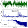 |
Fig. 1. Upper panel: Light curve of KIC 6876668. The solid black line corresponds to the 20-d moving average. Medium and bottom panels: LS analysis of the light curve for the whole frequency range (medium panel) and for the period range [30 d, 90 d] (bottom panel). Black arrows indicate the possible peaks of short-term cycles (with corresponding periods in days). The broad peaks around 0.18−0.2 d−1 show the rotation period of the star. The solid and dashed light blue lines give the background power level and the 10−6 FAP level, respectively. The vertical grey lines mark the separation between the frequency bins used to the determine the background power spectrum. |
The middle and bottom panels of Fig. 1 show the LS analysis of the data series. Stellar rotation is clearly seen in the frequency interval of 0.17−0.21 d−1. This interval is quite wide as it is typical for a rotation frequency of Kepler stars. Besides the rotation frequency, there are lower frequencies corresponding to periods of 47, 59, and 72 d. These periods are several times longer than the rotation period, which is entirely consistent with the length of the Rieger-type cycles on the Sun. The significance of these three power peaks is evaluated with the help of the mean background spectrum, computed with the quick_background function with nbin = 10; see Sect. 2 for more details. The middle and bottom panels of Fig. 1 show that the 47-d power peak has a FAP smaller than 10−6 and so can be considered as significant. The other two peaks, on the other hand, have a FAP above the 10−6 level and could in principle be discarded. They are also closer to the quarter duration of Kepler observations, which could introduce some modulation of instrumental origin. More specifically, the FAP of the three peaks is 3.2 × 10⁻⁷, 1.4 × 10⁻⁵ and 3.4 × 10⁻⁴.
We then performed a wavelet analysis to obtain an independent estimation of the significance of these power peaks and to see the evolution of the periodicities over time. The KIC 6876668 data are unequally spaced and contain gaps, so we interpolated them on a time grid with a uniform spacing of 0.02042 d (≈29 min, Kepler cadence). Figure 2 confirms the results obtained from the LS periodogram. First, this figure clearly shows the rotation period, Prot, above the 95% confidence level almost continuously throughout the four years of observation. Furthermore, the three peaks with periods of 47, 59, and 72 d are all above the 95% confidence level, and therefore we interpret them as physical variability of KIC 6876668. Moreover, the first peak with a period of about 43−48 d took place from about mid 2010 to the beginning of 2012. The next stronger peak, at a period of 56−58 d, was present in the middle of 2010 to the first half of 2012. Finally, the peak with a period of around 75 d was observed during 2010 and the beginning of 2011.
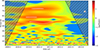 |
Fig. 2. Wavelet analysis of the KIC 6876668 light curve in the range 2−90 d. Short-term cycles at 43−48, 56−58, and 75 d are clearly seen. The Morlet mother function with η = 20 has been used (Torrence & Compo 1998). The white contours give the 95% confidence levels (Auchère et al. 2016). |
The multiple cycles observed in the light curve of KIC 6876668 may have a common occurrence on stars. Gurgenashvili et al. (2022) found similar cycles on the Kepler star KIC 2852336. It is important to compare the cycles to the periods observed in solar activity.
4. The Sun as a star in the cycle 23
The solar analogue of stellar light curves is the total solar irradiance (TSI). TSI has a significant impact on the Earth; therefore, it has been continuously recorded for almost 45 years through various missions.
To compare TSI to the light curve variations of KIC 6876668, we selected solar cycle 23. Although solar data, primarily sunspot records, extend back to the 17th century, comparing stellar light curves with other data, aside from solar irradiance, is not optimal. While some reconstruction models even extend back to the Maunder Minimum (Yeo et al. 2014, 2017; Wu et al. 2018; Krivova et al. 2010), we focused on observational data from SOHO/VIRGO (Fröhlich et al. 1995) and SORCE/TIM (Kopp et al. 2005) for recent cycles.
Figure 3 (upper panel) shows the TSI observations obtained by SOHO/VIRGO during solar cycle 23. The data shows a clear 11-year modulation as well as the modulation with shorter periods from several months to 1−1.5 yr. Note that we only discuss the peaks classified as short periods. Although the 1-yr periodicity is not usually considered a Rieger periodicity, we include it in our analysis for a comparison with the detected stellar cycles.
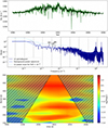 |
Fig. 3. Upper panel: Total irradiance of the Sun during cycle 23 based on SOHO/VIRGO data. The solid black line corresponds to the 30-d moving average. Medium panel: LS analysis of the TSI data for the whole frequency range. The meaning of lines and arrows are the same as in Fig. 1. Bottom panel: Wavelet analysis of the TSI in the range 150−450 d. The significance level of all power peaks is below 5% and for this reason the confidence level contours are not plotted. We only consider peaks that are consistent with Rieger periodicity and 1-year cycle. Longer period features are not classified as Rieger-type cycles. |
The medium and bottom panels of the figure display the LS and wavelet spectra of the time series in the range of 150−450 d. Three well-defined periods are seen in both panels. The shortest period corresponds to 185 d, which is the Rieger-type periodicity already reported by Gurgenashvili et al. (2021). This period is seen in the interval between 1998 and 2004, i.e. during the maximum of cycle 23.
The second periodicity corresponds to ∼240 d and it also takes place at the maximum of the solar cycle. A similar period is also reported in the daily sunspot data of GRO (Gachechiladze et al. 2019). The third, most powerful peak corresponds to a period of about 1 year and is continuously seen during the whole cycle. The quasi-annual cycle was already reported in other solar activity indices such as sunspots, (Wolff 1983; Ichimoto et al. 1985; Bai 1987; Lean & Brueckner 1989; Oliver et al. 1992; Gachechiladze et al. 2019). Table 2 shows the multiple cycles in the total irradiance of the Sun and in the light curve of the Kepler star.
Rotation periods and Rieger periods for the Sun and KIC 6876668.
We see that, although the solar periods around 185, 240, and 380 d are well established in cycle 23 from various activity indices, in TSI the LS power lies below the 10−6 FAP threshold line (see the middle panel of Fig. 3). At the same time, they appear at a confidence level of < 5% in the wavelet spectrum (see the bottom panel). This implies that the TSI is not a good solar indicator for detecting these periods with enough confidence. On the other hand, the periodicities of 47, 59, and 73 d have been confidently assessed in the light curve of the KIC 6876668 star. This allows us to conclude that these must be strong periodicities.
When comparing the significance of the periodicities in the KIC 6876668 data and in the TSI data, one must be aware that the number of samples per period is quite different in the two datasets. In the first one, with a cadence around 0.0204-d, there are ≃2280 and ≃3540 samples per period for the periods of 46.6 and 72.3-d, respectively. On the other hand, the TSI cadence is 1-d; hence, the number of samples per period for the shortest and longest TSI periodicities of Table 2 are ≃185 and ≃382, respectively. In view of the discrepancy between the number of samples per period, we retained only one KIC 6876668 data value out of ten and repeated the spectral analysis, obtaining results that are very much the same as those in Figs. 1 and 2: the three main periodicities have a very similar period and confidence level,  d,
d,  d, and
  d (see Fig. 4). This leads us to conclude that the strong, statistically significant periodicities found in the KIC 6876668 data are not caused by the high cadence and that they are true periodicities of the light curve of this star.
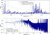 |
Fig. 4. Same as the middle and bottom panels of Fig. 1; however, the spectral analysis was repeated by retaining only one out of every ten stellar data values. The three main periodicities had nearly identical periods and confidence levels. |
5. Solar versus stellar Rieger cycles
One can note that the three periods seen on Fig. 3 are quite similar to the periods of Fig. 2. The comparison between solar and stellar Rieger cycles is presented in Table 2. Simple estimations show that the ratios of the cyclic and the rotation periods for the Sun and the star have almost similar values. Therefore, the cycles are probably excited by the same mechanism. It is believed that the Rieger cycles in solar activity are excited due to magnetic Rossby waves in the dynamo layer (Zaqarashvili et al. 2010, 2021). Therefore, the multiple cycles may correspond to the different harmonics of Rossby waves (Gachechiladze et al. 2019).
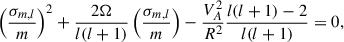
The solutions and dispersion relations of magnetic Rossby waves depend on the latitudinal structure of toroidal magnetic field. In the case of a simple Malkus profile (symmetric and homogeneous with latitude), the solutions are in terms of associated Legendre polynomials and the dispersion relation is (in the rotating frame)
 (1)
(1)
where σm, l is the wave frequency of (m, l) harmonic, Ω is the angular frequency of the rotating stellar layer, R is the distance from the centre,  is the Alfvén speed (B is the magnetic field strength and ρ is the density), and m (corresponding to the toroidal wave number, i.e. the number of zeros in the toroidal direction) and l (corresponding to the total number of zeros on the sphere) are the angular order and degree of spherical harmonics. For a more complex magnetic profile that resembles the dynamo field, having maxima at middle latitudes and a changing sign at the equator (anti-symmetric with latitudes), the solution of magnetic Rossby waves is in terms of spheroidal wave functions with a more complex dispersion relation (Gachechiladze et al. 2019).
Angular frequency, density, and the distance of the dynamo layer from the centre is more or less known for the Sun. Therefore, observed oscillation frequencies can be identified with σm, l estimating the corresponding magnetic field strength, B. It is known that the most unstable harmonic of magnetic Rossby waves is for m = 1 (Zaqarashvili et al. 2010); therefore, observed oscillation periods can be identified with magnetic Rossby wave harmonics having m = 1, but different values of l. Figure 5 shows the periods of fast magnetic Rossby wave harmonics with (m, l) = (1, 4), (1, 5), (1, 6), (1, 7) versus the magnetic field strength in the dynamo layer for the anti-symmetric profile of the field. The observed periods in TSI are marked with points. It is seen that the observed periods correspond to the harmonics of (1, 4), (1, 5), (1, 7) in the case of the magnetic field strength of ∼10 kG. We do not consider the (m = 1, l = 6) harmonic on Fig. 5. For the magnetic field of 10 kG, the period corresponding to the harmonic must be around 340 d. No significant peak is seen near that period on the spectrum. However, we still see a small peak near this value in the LS spectrum. The wavelet spectrum also displays a peak near that period, but it is masked by the stronger 382-d periodicity. Therefore, we consider (1, 6) signal as insignificant and consequently focus on the harmonics that are more clearly detected. The (m = 1, l = 6) harmonic is antisymmetric with regards to the equator; therefore, the contributions of the northern and southern hemispheres may cancel each other out in TSI, so we see only the small peak. Anyway we prefer to work only with the peaks, which are more significant in the power spectra. Therefore, 10 kG magnetic field strength in the dynamo layer will lead to the observed multiple periods in solar activity.
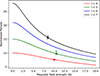 |
Fig. 5. Normalised periods of magneto-Rossby wave spherical harmonics vs dynamo magnetic field strength for the solar dynamo layer. Curves with different colours correspond to the harmonic with m = 1 and l = 4, 5, 6, 7, respectively. The harmonics with m = 1 and l = 4, 5, 7, correspond to the observed periods in the case of solar dynamo field strength of 10 kG. Note that no clear detection is seen for the m = 1, l = 6 harmonic. |
Now let us consider the cycles in the light curve of KIC 6876668. This star is considered as a young solar analogue in Kepler catalogues and as a subgiant in Gaia data. In the first case, the parameters used in Eq. (1) (the distance of the base of the convection zone from the centre, R, density near the base of the convection zone, ρ) can be taken as those of the Sun. In the second case, one can follow the evolution of one solar mass star and take the parameters from the model near the subgiant stage. Different latitudinal profiles of the toroidal magnetic field affect the dispersion relation of magnetic Rossby waves, and therefore the periods of spherical harmonics. Consequently, the magnetic field strengths inferred from Rossby mode analysis may carry an estimated systematic uncertainty of about 20−30%. However, this does not influence our identification of the (m, l) modes or the overall physical interpretation. On the other hand, if the latitudinal structure of the surface magnetic field is known from the multiple Zeeman Doppler imaging studies (Reiners 2012; Donati & Landstreet 2009), then the uncertainty can be significantly reduced. We use the model of Iben (1967), but other recent models show basically similar values. Figure 1 of Iben (1967) displays the luminosity versus surface temperature of stars near solar mass during post-main-sequence evolution. Four times the solar luminosity of a solar-mass star is achieved at the position marked by 11. The corresponding internal structure of the star is plotted on Fig. 10 in Iben (1967). The radius of the star is 2.2 Rsun, where the base of the convection zone corresponds to 0.7 of the stellar radius, i.e. R = 1.54 Rsun. At the same time, the density near the base of the convection zone is 0.06 g/cm3. We use these parameters to plot the figure for stellar magneto-Rossby waves similar to Fig. 5.
Figure 6 shows the periods of fast magnetic Rossby wave harmonics with (m, l) = (1, 4), (1, 5), (1, 6) versus the magnetic field strength in the dynamo layer for the anti-symmetric profile of the field. The observed periods in stellar light curve are marked with points. The observed periods correspond to the harmonics of (1, 4), (1, 5), (1, 6) in the case of magnetic field strength of ∼30−35 kG. Hence, ∼30−35 kG magnetic field strength in the dynamo layer of the star will lead to the observed multiple periods in the light curve. The analysis shows that a rapidly rotating star has a much stronger dynamo field strength than the Sun, as expected.
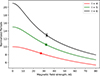 |
Fig. 6. Normalised periods of magneto-Rossby wave spherical harmonics vs dynamo magnetic field strength for the stellar dynamo layer. Curves with different colours correspond to the spherical harmonic with m = 1 and l = 4, 5, 6, respectively. The harmonics with m = 1 and l = 4, 5, 6, correspond to the observed periods in the case of stellar dynamo field strength of 30−35 kG. |
6. Discussion and conclusion
Rieger periodicity has been observed in many activity indices of the Sun over the past several decades. The periodicity is enigmatic; its value changes from cycle to cycle according to the cycle strength. The periodicity usually appears during cycle maxima and disappears in other activity phases. Recent studies showed that the Rieger periodicity is anti-correlated with solar cycle strength, so that the stronger cycles display shorter periods and vice versa (Gurgenashvili et al. 2016).
Recently, Gurgenashvili et al. (2022) found an interesting solar-type star with a rotation period of 9.5 d and a Rieger period of about 61 d. It was revealed that the rotation period of this star is three times shorter than that of the Sun. At the same time, the estimated strength of its dynamo (from Eq. (1)) magnetic field was found to be about three times greater than that of our Sun. This led to the suggestion that the ratio of Ω/B is constant throughout stellar evolution. Therefore, it is of importance to search for Rieger-type periods in other stars and to test the hypothesis.
In this paper, we continue the case study of Kepler stars and show that a young, bright counterpart of the Sun, KIC 6876668, with a rotation period of around 5−6 d (Reinhold et al. 2013; McQuillan et al. 2014), displays multiple cycles in the light curve. The periods of the cycles are 47, 59, and 72 d and are comparable to the range of Rieger periods in the Sun. To check the reliability of the periods, we used several methods. First, we checked the star through other space missions, such as Gaia and TESS, to obtain additional data. Through Gaia, we determined that this star has no companion star at a close distance that could affect these periods. Second, we used wavelet analysis to examine when these periods appeared in the stellar light curves. The first and the last quarters of Kepler are considered relatively unreliable; therefore, observed periods should be outside these quarters. Indeed, wavelet analysis showed that these periods are located in the interval of 2010−2012; hence, the obtained periods can be considered to be reliable.
In order to compare the obtained periods to the solar counterparts, we analysed TSI data in cycle 23 and found three main periods: 185 d, 240 d, and an approximately 1-yr period. If one compares the observed cycles in solar and stellar light curves normalised by the corresponding rotation periods, one can find the ratios of 7.6, 9.7, and 15.6 for the Sun, and the ratios of 8.3, 10.5, and 12.9 for the star (see Table 2). There is a clear correspondence between the multiple cycles of the Sun and those of the star. We tried to interpret the multiple cycles in solar and stellar light curves as magnetic Rossby waves in the dynamo layer. The theory of magnetic Rossby waves suggests that the periods in stellar light curves can be interpreted as the spherical harmonics with m = 1 and l = 4, 5, 6 in the case of a stellar dynamo field of 30−35 kG. On the other hand, the periods in solar total irradiance can be interpreted as the spherical harmonics with m = 1 and l = 4, 5, 7 in the case of a solar dynamo field of 10 kG. As the stellar rotation period of KIC 6876668 is approximately 4.5 times shorter than the solar rotation period, one might conclude that Ωstar/Ωsun ∼ Bstar/Bsun ∼ 4, and hence
 (2)
(2)
which coincides with the result found by Gurgenashvili et al. (2022). Hence, our analysis shows that the ratio of stellar angular frequency and the dynamo field strength is the same for stars with solar mass at different phases of evolution. Therefore, the ratio may remain constant throughout the stellar evolution. On the other hand, Reiners et al. (2022) derived the relationship between the average surface field and the Rossby number as B ∼ Ro−1.26 ± 0.10 for red dwarfs, which is slightly different from our result. The slight difference between the two results can be mainly explained by two reasons. First, the difference could be caused by the different spectral types of sample stars. Reiners et al. (2022) considered light red dwarfs, while we considered stars with solar mass. Second, Reiners et al. (2022) considered the relation between the surface magnetic field and angular frequency, while we estimated the dynamo magnetic field strength, which is actually based below the convection zone of Sun-like stars.
The possibility of probing magnetic fields at subsurface layers would shed light on the question of magnetic field generation and flux emergence. An interesting question is how the subsurface fields scale with rotation and whether the surface fields are reflecting the field strengths at lower layers or are only parts of the subsurface fields of which different fractions are visible at the surface. A larger sample of stars with measurements of short-term cycles will help us to measure the depth dependence of stellar magnetic fields.
The consistent relationship observed between the Rieger period and the rotation period in KIC 6876668’s activity suggests that the physical processes occurring in its interior, which drive stellar cycles, are similar to those in the Sun. By studying young solar analogues, we can gain critical insights into the early stages of solar magnetic activity and its subsequent evolution. Our investigation into the magnetic cycles of Sun-like stars has revealed that Rieger cycles are not unique to the Sun and may be quite common among similar stars. The study of young stars allows us to compare their activity with that of the Sun, helping us understand how stellar cycles evolve over time.
Ultimately, the results for KIC 6876668 enhance our understanding of the connection between stellar rotation and magnetic activity. Future research should encompass a broader range of solar analogues to explore the universality and significance of these phenomena for Sun-like stars at different stages of evolution.
Acknowledgments
This work was supported by Shota Rustaveli National Science Foundation of Georgia (SRNSFG) [YS-24-088]. TVZ was supported by the Austrian Science Fund (FWF) project PAT7550024. This publication is part of the R+D+i project PID2023-147708NB-I00, financed by MCIN/AEI/10.13039/501100011033. The authors gratefully acknowledge advice and comments by Dr. Sylvain Breton that helped to improve the data analysis of the present work. This research was supported by the International Space Science Institute (ISSI) in Bern, through ISSI International Team project 24-629 (Multiscale variability in solar and stellar magnetic cycles).
References
- Arkhypov, O. V., & Khodachenko, M. L. 2021, A&A, 651, A28 [NASA ADS] [CrossRef] [EDP Sciences] [Google Scholar]
- Arkhypov, O. V., Khodachenko, M. L., Lammer, H., et al. 2015, ApJ, 807, 109 [NASA ADS] [CrossRef] [Google Scholar]
- Astropy Collaboration (Robitaille, T. P., et al.) 2013, A&A, 558, A33 [NASA ADS] [CrossRef] [EDP Sciences] [Google Scholar]
- Astropy Collaboration (Price-Whelan, A. M., et al.) 2018, AJ, 156, 123 [Google Scholar]
- Astropy Collaboration (Price-Whelan, A. M., et al.) 2022, ApJ, 935, 167 [NASA ADS] [CrossRef] [Google Scholar]
- Auchère, F., Froment, C., Bocchialini, K., et al. 2016, ApJ, 825, 110 [CrossRef] [Google Scholar]
- Baglin, A., Auvergne, M., Barge, P., Deleuil, M., & Michel, E. 2008, Proc. Int. Astron. Union, 4, 71 [NASA ADS] [CrossRef] [Google Scholar]
- Bai, T. 1987, ApJ, 318, L85 [Google Scholar]
- Bai, T., & Cliver, E. H. 1990, ApJ, 363, 299 [Google Scholar]
- Bai, T., & Sturrock, P. A. 1987, Nature, 327, 601 [NASA ADS] [CrossRef] [Google Scholar]
- Bai, T., & Sturrock, P. A. 1991, Nature, 350, 141 [Google Scholar]
- Baliunas, S. L., Donahue, R. A., Soon, W. H., et al. 1995, ApJ, 438, 269 [Google Scholar]
- Ballester, J. L., Oliver, R., & Carbonell, M. 2002, ApJ, 566, 505 [NASA ADS] [CrossRef] [Google Scholar]
- Barnes, S. A. 2010, ApJ, 722, 222 [Google Scholar]
- Berger, T. A., Huber, D., Gaidos, E., & van Saders, J. L. 2018, ApJ, 866, 99 [NASA ADS] [CrossRef] [Google Scholar]
- Bonomo, A. S., & Lanza, A. F. 2012, A&A, 547, A37 [NASA ADS] [CrossRef] [EDP Sciences] [Google Scholar]
- Boro Saikia, S., Marvin, C. J., Jeffers, S. V., et al. 2018, A&A, 616, A108 [NASA ADS] [CrossRef] [EDP Sciences] [Google Scholar]
- Borucki, W., Koch, D., Basri, G., et al. 2010, Science, 327, 977 [CrossRef] [PubMed] [Google Scholar]
- Breton, S. N., Lanza, A. F., & Messina, S. 2024a, A&A, 682, A67 [NASA ADS] [CrossRef] [EDP Sciences] [Google Scholar]
- Breton, S. N., Lanza, A. F., Messina, S., et al. 2024b, A&A, 689, A229 [NASA ADS] [CrossRef] [EDP Sciences] [Google Scholar]
- Carbonell, M., & Ballester, J. L. 1990, A&A, 238, 377 [NASA ADS] [Google Scholar]
- Carbonell, M., & Ballester, J. L. 1992, A&A, 255, 350 [NASA ADS] [Google Scholar]
- Donati, J. F., & Landstreet, J. D. 2009, ARA&A, 47, 333 [Google Scholar]
- Foster, G. 1996, AJ, 112, 1709 [NASA ADS] [CrossRef] [Google Scholar]
- Fröhlich, C., Romero, J., Roth, H., et al. 1995, Sol. Phys., 162, 101 [Google Scholar]
- Gachechiladze, T., Zaqarashvili, T. V., Gurgenashvili, E., et al. 2019, ApJ, 874, 162 [NASA ADS] [CrossRef] [Google Scholar]
- García, R. A., Mathur, S., Salabert, D., et al. 2010, Science, 329, 1032 [Google Scholar]
- Gilliland, R. L., Chaplin, W. J., Jenkins, J. M., Ramsey, L. W., & Smith, J. C. 2015, AJ, 150, 133 [Google Scholar]
- Gurgenashvili, E., Zaqarashvili, T. V., Kukhianidze, V., et al. 2016, ApJ, 826, 55 [NASA ADS] [CrossRef] [Google Scholar]
- Gurgenashvili, E., Zaqarashvili, T. V., Kukhianidze, V., et al. 2017, ApJ, 845, 137 [NASA ADS] [CrossRef] [Google Scholar]
- Gurgenashvili, E., Zaqarashvili, T. V., Kukhianidze, V., et al. 2021, A&A, 653, A146 [NASA ADS] [CrossRef] [EDP Sciences] [Google Scholar]
- Gurgenashvili, E., Zaqarashvili, T. V., Kukhianidze, V., et al. 2022, A&A, 660, A33 [NASA ADS] [CrossRef] [EDP Sciences] [Google Scholar]
- Iben, I. 1967, ApJ, 147, 624 [NASA ADS] [CrossRef] [Google Scholar]
- Ichimoto, K., Kubota, J., Suzuki, M., et al. 1985, Nature, 316, 422 [Google Scholar]
- Kopp, G., Lawrence, G., & Rottman, G. 2005, Sol. Phys., 230, 129 [NASA ADS] [CrossRef] [Google Scholar]
- Krivova, N. A., Vieira, L. E. A., & Solanki, S. K. 2010, J. Geophys. Res., 115, A12112 [Google Scholar]
- Lanza, A. F., Pagano, I., Leto, G., et al. 2009, A&A, 493, 193 [NASA ADS] [CrossRef] [EDP Sciences] [Google Scholar]
- Lanza, A. F., Netto, Y., Bonomo, A. S., et al. 2019, A&A, 626, A38 [NASA ADS] [CrossRef] [EDP Sciences] [Google Scholar]
- Lean, J. L. 1990, ApJ, 363, 718 [Google Scholar]
- Lean, J. L., & Brueckner, G. E. 1989, ApJ, 337, 568 [Google Scholar]
- Lomb, N. R. 1976, Ap&SS, 39, 447 [Google Scholar]
- Lou, Y.-Q. 2000, ApJ, 540, 1102 [NASA ADS] [CrossRef] [Google Scholar]
- McQuillan, A., Mazeh, T., & Aigrain, S. 2014, ApJS, 211, 24 [Google Scholar]
- Mengel, M. W., Fares, R., Marsden, S. C., et al. 2016, MNRAS, 459, 4325 [NASA ADS] [CrossRef] [Google Scholar]
- Metcalfe, T. S., Basu, S., Henry, T. J., et al. 2010, ApJ, 723, L213 [NASA ADS] [CrossRef] [Google Scholar]
- Mittag, M., Robrade, J., Schmitt, J. H. M. M., et al. 2017, A&A, 600, A119 [NASA ADS] [CrossRef] [EDP Sciences] [Google Scholar]
- Mittag, M., Schmitt, J. H. M. M., Hempelmann, A., & Schroeder, K.-P. 2019, A&A, 621, A136 [NASA ADS] [CrossRef] [EDP Sciences] [Google Scholar]
- Nielsen, M. B., Gizon, L., Schunker, H., & Karoff, C. 2013, A&A, 557, L10 [NASA ADS] [CrossRef] [EDP Sciences] [Google Scholar]
- Noyes, R. W., Weiss, N. O., & Vaughan, A. H. 1984, ApJ, 287, 769 [Google Scholar]
- Oliver, R., Carbonell, M., & Ballester, J. L. 1992, Sol. Phys., 137, 141 [Google Scholar]
- Oliver, R., Ballester, J. L., & Boudin, F. 1998, Nature, 394, 552 [NASA ADS] [CrossRef] [Google Scholar]
- Rauer, H., Aerts, C., Cabrera, J., et al. 2025, Exp. Astron., 59, 26 [Google Scholar]
- Reiners, A. 2012, Liv. Rev. Sol. Phys., 9, 1 [Google Scholar]
- Reiners, A., Shulyak, D., Käpylä, P. J., et al. 2022, A&A, 662, A41 [NASA ADS] [CrossRef] [EDP Sciences] [Google Scholar]
- Reinhold, T., Reiners, A., & Basri, G. 2013, A&A, 560, A4 [NASA ADS] [CrossRef] [EDP Sciences] [Google Scholar]
- Reinhold, T., Shapiro, A. I., Solanki, S. K., & Basri, G. 2024, A&A, 678, A24 [Google Scholar]
- Ricker, G. R., Winn, J. N., Vanderspek, R., et al. 2014, Proc. SPIE, 9143, 914320 [Google Scholar]
- Rieger, E., Share, G. H., Forrest, D. J., et al. 1984, Nature, 312, 623 [Google Scholar]
- Saar, S. H., & Baliunas, S. L. 1992, ASP Conf. Ser., 27, 197 [NASA ADS] [Google Scholar]
- Saar, S. H., & Brandenburg, A. 1999, ApJ, 524, 295 [NASA ADS] [CrossRef] [Google Scholar]
- Santos, A. R. G., García, R. A., Mathur, S., et al. 2019, ApJS, 244, 21 [Google Scholar]
- Santos, A. R. G., Breton, S. N., Mathur, S., & García, R. A. 2021, ApJS, 255, 17 [NASA ADS] [CrossRef] [Google Scholar]
- Scargle, J. D. 1982, ApJ, 263, 835 [Google Scholar]
- Schmitt, J. H. M. M., & Mittag, M. 2017, A&A, 600, A120 [NASA ADS] [CrossRef] [EDP Sciences] [Google Scholar]
- Simonian, G. V. A., Pinsonneault, M. H., & Terndrup, D. M. 2019, ApJ, 871, 174 [Google Scholar]
- Sturrock, P. A., Bertello, L., Fischbach, E., et al. 2013, APh, 42, 62 [Google Scholar]
- Torrence, C., & Compo, G. P. 1998, Bull. Am. Meteorol. Soc., 79, 61 [Google Scholar]
- VanderPlas, J. T. 2018, ApJS, 236, 16 [Google Scholar]
- Wilson, O. C. 1978, ApJ, 226, 379 [Google Scholar]
- Wolff, C. L. 1983, ApJ, 264, 667 [Google Scholar]
- Wolff, C. L. 1992, SoPh, 142, 187 [Google Scholar]
- Wu, C.-J., Krivova, N. A., Solanki, S. K., & Usoskin, I. G. 2018, A&A, 620, A120 [NASA ADS] [CrossRef] [EDP Sciences] [Google Scholar]
- Yeo, K. L., Krivova, N. A., Solanki, S. K., & Glassmeier, K. H. 2014, A&A, 570, A85 [NASA ADS] [CrossRef] [EDP Sciences] [Google Scholar]
- Yeo, K. L., Krivova, N. A., & Solanki, S. K. 2017, J. Geophys. Res.: Space Phys., 122, 3888 [NASA ADS] [CrossRef] [Google Scholar]
- Zaqarashvili, T. V., & Gurgenashvili, E. 2018, Front. Astron. Space Sci., 5, 7 [CrossRef] [Google Scholar]
- Zaqarashvili, T. V., Carbonell, M., Oliver, R., & Ballester, J. L. 2010, ApJ, 709, 749 [NASA ADS] [CrossRef] [Google Scholar]
- Zaqarashvili, T. V., Albekioni, M., Ballester, J. L., et al. 2021, Space Sci. Rev., 217, 15 [Google Scholar]
Data sources: Reinhold et al. (2013): https://cdsarc.cds.unistra.fr/viz-bin/qcat?J/A+A/560/A4, Nielsen et al. (2013): https://cdsarc.cds.unistra.fr/viz-bin/qcat?J/A+A/557/L10, McQuillan et al. (2014): https://vizier.u-strasbg.fr/viz-bin/VizieR?-source=J/ApJS/211/24, Reinhold et al. (2024): https://cdsarc.cds.unistra.fr/viz-bin/cat/J/A+A/678/A24, Santos et al. (2019): https://cdsarc.cds.unistra.fr/viz-bin/cat/J/ApJS/244/21, Santos et al. (2021): https://cdsarc.cds.unistra.fr/viz-bin/cat/J/ApJS/255/17
All Tables
All Figures
|
Fig. 1. Upper panel: Light curve of KIC 6876668. The solid black line corresponds to the 20-d moving average. Medium and bottom panels: LS analysis of the light curve for the whole frequency range (medium panel) and for the period range [30 d, 90 d] (bottom panel). Black arrows indicate the possible peaks of short-term cycles (with corresponding periods in days). The broad peaks around 0.18−0.2 d−1 show the rotation period of the star. The solid and dashed light blue lines give the background power level and the 10−6 FAP level, respectively. The vertical grey lines mark the separation between the frequency bins used to the determine the background power spectrum. |
| In the text | |
|
Fig. 2. Wavelet analysis of the KIC 6876668 light curve in the range 2−90 d. Short-term cycles at 43−48, 56−58, and 75 d are clearly seen. The Morlet mother function with η = 20 has been used (Torrence & Compo 1998). The white contours give the 95% confidence levels (Auchère et al. 2016). |
| In the text | |
|
Fig. 3. Upper panel: Total irradiance of the Sun during cycle 23 based on SOHO/VIRGO data. The solid black line corresponds to the 30-d moving average. Medium panel: LS analysis of the TSI data for the whole frequency range. The meaning of lines and arrows are the same as in Fig. 1. Bottom panel: Wavelet analysis of the TSI in the range 150−450 d. The significance level of all power peaks is below 5% and for this reason the confidence level contours are not plotted. We only consider peaks that are consistent with Rieger periodicity and 1-year cycle. Longer period features are not classified as Rieger-type cycles. |
| In the text | |
|
Fig. 4. Same as the middle and bottom panels of Fig. 1; however, the spectral analysis was repeated by retaining only one out of every ten stellar data values. The three main periodicities had nearly identical periods and confidence levels. |
| In the text | |
|
Fig. 5. Normalised periods of magneto-Rossby wave spherical harmonics vs dynamo magnetic field strength for the solar dynamo layer. Curves with different colours correspond to the harmonic with m = 1 and l = 4, 5, 6, 7, respectively. The harmonics with m = 1 and l = 4, 5, 7, correspond to the observed periods in the case of solar dynamo field strength of 10 kG. Note that no clear detection is seen for the m = 1, l = 6 harmonic. |
| In the text | |
|
Fig. 6. Normalised periods of magneto-Rossby wave spherical harmonics vs dynamo magnetic field strength for the stellar dynamo layer. Curves with different colours correspond to the spherical harmonic with m = 1 and l = 4, 5, 6, respectively. The harmonics with m = 1 and l = 4, 5, 6, correspond to the observed periods in the case of stellar dynamo field strength of 30−35 kG. |
| In the text | |
Current usage metrics show cumulative count of Article Views (full-text article views including HTML views, PDF and ePub downloads, according to the available data) and Abstracts Views on Vision4Press platform.
Data correspond to usage on the plateform after 2015. The current usage metrics is available 48-96 hours after online publication and is updated daily on week days.
Initial download of the metrics may take a while.