© The Authors 2026

1 Introduction

In scientific research, any measured data needs to be tested against a suitable hypothesis. As such, robust statistical techniques are indispensable for parameter estimation and model comparison. Science frequently faces the challenge of characterising probability distributions arising from complex, high-dimensional models ridden with nuisance parameters, uncertainties, and degeneracies. Markov chain Monte Carlo (MCMC) methods are widely recognised as a vital tool in many areas of science. They enable researchers to characterise parameter uncertainties precisely and compare models rigorously. Research areas that rely on precise inference, such as phylogenetics (Rannala & Yang 1996; Drummond et al. 2002), physio-chemistry (Hansmann 1997; Sugita & Okamoto 1999), gravitational waves (van der Sluys et al. 2008; Veitch et al. 2015), and exoplanet discovery (Jenkins et al. 2020; Vines et al. 2023), benefit from the flexibility of MCMC techniques to explore difficult posterior landscapes.

Early exoplanet radial-velocity (RV) detections were often confirmed by identifying significant peaks in periodograms – in which false-alarm probabilities were calculated to establish the significance of a planetary candidate – and performing nonlinear least-squares fitting for Keplerian orbits. Such was the case for 51 Pegasi b (Mayor & Queloz 1995) – the first exoplanet around a Sun-like star – and for the many Jovian planets that quickly followed this discovery (Gonzalez 1997; Marcy & Butler 2000).

However, as RV data grew and multi-planet systems became common, more sophisticated statistical tools were needed to extract the more difficult exoplanet signals, which could be subtle, degenerate, and embedded in considerable noise. This led to the introduction of MCMC methods (Ford et al. 2005), revolutionising exoplanet RV fitting with robust estimation of orbital parameters with realistic uncertainties, even for nonlinear parameters (such as eccentricity and longitude of periastron). Far from perfect, MCMC still has its caveats. Poorly tuned chains could wander slowly or get trapped in local maxima.

To thoroughly explore multi-modal parameter spaces (common in multi-planet systems, for example), Gregory (2005) pioneered the use of the parallel tempering (PT) MCMC method (Swendsen & Wang 1986; Earl & Deem 2005) in relation to RV-signal detection and characterisation. This approach runs several chains in parallel to sample different powers (a temperature ladder) of the posterior distribution, each tempered to a different level. Hotter chains traverse the parameter space with more freedom, while colder chains sample the fine details. Inter-chain communication allows the sampler to explore distant high-probability nodes with ease. Furthermore, PT enables the algorithm to estimate the marginalised posterior (or evidence), a crucial quantity for model comparison. Gregory (2005) shows that this method is capable of efficiently exploring all regions of the phase space, lessening the burden of multi-modality. However, this early implementation was not capable of estimating the evidence reliably without a huge performance loss.

The affine-invariant ensemble samplers (Goodman & Weare 2010) also found their way into the exoplanet domain (Hou et al. 2012a). This MCMC variant, instead of a single chain, utilises an ensemble of ‘walkers’, drawing multiple samples per step, making the sampler insensitive to parameter covariances, and thus providing an enormous computational performance boost.

As an extra Keplerian in one’s model can always fit noise, efforts turned to providing an accurate model comparison framework, leading to the usage of nested sampling (NS) algorithms (Skilling 2004) to calculate the Bayesian evidence for competing models (with differing number of planets or noise models), allowing one to select the most likely model (Feroz & Hobson 2008; Feroz et al. 2011). Building on NS, dynamic NS (DNS, Higson et al. 2019; Speagle 2020) introduces an adaptive allocation of ‘sampling effort’ to higher-probability areas of the phase space, further increasing the efficiency of reaching the target evidence precision, finding use in RV fitting (Diamond-Lowe et al. 2020).

MCMC excels in parameter posterior estimation, yielding reliable uncertainties, even for complex or correlated parameters. However, while evidence estimation is certainly possible under this algorithm, it is as a by-product of the posterior exploration. Therefore, increasing the accuracy of the evidence estimation does not necessarily translate into increased posterior accuracy, while carrying a substantial computational burden. On the other hand, NS is primarily designed for efficient evidence estimation by systematically shrinking the likelihood volume. As a by-product, it provides posterior samples, which can be used to model the parameter posteriors. Consequently, this method inherently does not provide as many samples from the parameter distribution as a well-tuned MCMC, conveying less precise parameter estimates.

This work presents reddemcee¹, an adaptive PT MCMC Python algorithm for any scientific-sampling-related endeavour that handles complex, high-dimensional, multi-modal posteriors, with several competing models. Leveraging five different automated tuning strategies for the temperature ladder – two classic ones, uniform swap acceptance, and posterior area overlap; and three new implementations based on average energy differences, the system’s specific heat, and the swap mean distance (SMD) – while providing original adaptations for evidence estimation, such as the stepping stones algorithm (SS, Xie et al. 2011) with a per-stone geometric-bridge, thermodynamic integration (TI, Gelman & Meng 1998) enhanced by curvature-aware interpolation, and a novel hybrid approach.

2 Bayesian framework

A full description of Bayesian inference and MCMC methods is beyond the scope of this manuscript, and we therefore refer the reader to Gelman et al. (2004). Nonetheless, a summary of essential concepts is provided.

Bayesian inference generally consists of depicting the posterior probability distribution over the parameters θ ∈ Θ of the hypothesise model, M, depicting some known measured data, D: $$p(\theta \mid D,M)=\frac{p(\theta \mid M)\cdot p(D\mid \theta ,M)}{p(D\mid M)},$$(1) where p(θ | M) corresponds to the prior distribution, p(D | θ, M) to the likelihood function, and p(D | M) to the marginalised likelihood, frequently denoted as the Bayesian evidence, 𝒵, or simply ‘evidence’ (as it is in this manuscript). Throughout this work, proper priors are assumed (∫_Θ p(θ | M) = 1), so the evidence is well defined and finite.

The evidence quantifies the overall support for model M and is crucial for Bayesian model comparison. However, the evidence integral generally has no closed-form solution and must be estimated numerically (Oaks et al. 2018). The MCMC methods, while excelling at drawing samples from the posterior, do not directly provide 𝒵.

Within MCMC methods, several evidence-estimation techniques have been developed (Maturana-Russel et al. 2019). For PT MCMC, two common approaches are TI (Gelman & Meng 1998) and stepping stones (Xie et al. 2011). How PT works and how TI and SS leverage the tempered ensemble to estimate the evidence are briefly outlined below.

2.1 Parallel tempering MCMC

Parallel tempering MCMC runs an ensemble of B parallel chains, each sampling a different power of the posterior distribution (at a different temperature, T_i; Swendsen & Wang 1986; Earl & Deem 2005; Miasojedow et al. 2013). The inverse of the temperature is $\beta =\frac{1}{T}$, with 1 = β₁ > β₂ > … > β_B−1 > β_B ≥ 0, and the full chain ${\overline{X}}_t=\left(X_t^{\left({\beta }_1\right)},\dots ,X_t^{\left({\beta }_B\right)}\right)$. By convention, β₁ = 1 for the cold chain (sampling the original posterior) and β_B ≈ 0 for the hottest chain (sampling a highly flattened landscape, approaching the prior as β_B → 0). Each chain, $X_t^{\left({\beta }_i\right)}$, samples a tempered posterior where the likelihood has been raised to the power β_i, $${{\beta }_i}_{}(\theta )=\frac{\text{Π}\cdot {ℒ}^{{\beta }_i}}{{\mathcal{Z}}_{{\beta }_i}},$$(2) where ${{\beta }_i}_{}(\theta )$ is the posterior distribution , Π the prior, ${ℒ}^{{\beta }_i}$ the tempered likelihood, and $Z_{{\beta }_i}$ the evidence.

In 𝒫_β(θ), hotter temperatures flatten and broaden peaks, reducing the risk of getting trapped in local maxima, and effectively making the posterior easier to sample. As such, hot chains are able to rapidly sample a large portion of the parameter space, whilst cold chains provide precise local sampling. By allowing chains at different temperatures to swap states, PT achieves a fast, thorough sampling of the posterior. Swaps in PT are implemented with a Metropolis-like acceptance rule. The pairwise swap (Goggans & Chi 2004), which is when two adjacent chains $\left(X_t^{\left({\beta }_i\right)},X_t^{\left({\beta }_{i+1}\right)}\right)$ propose to switch states, is accepted with probability $$A_{i,i+1}=\min \left(0,-\text{Δ}\ln {ℒ}^{{\beta }_i}\cdot \text{Δ}{\beta }_i\right)$$(3) where ∆ln ${ℒ}^{{\beta }_i}$ is the log-likelihood difference between the two chain states. This criterion (derived by simplifying the detailed balance condition for swapping two Boltzmann-distributed ensembles) shows that swaps are more probable when a high-likelihood state from a hotter chain is proposed for a colder chain. Without adjacent posteriors overlapping enough to allow regular swaps, efficiency plummets. By tuning the temperature ladder (the set of β_i values), PT aims to maintain a reasonably high swap-acceptance rate (SAR) across all adjacent pairs, ensuring a thorough exploration of the posterior landscape and providing a natural framework for estimating the evidence, 𝒵, via the ladder of tempered distributions.

Although our APT implementation does not provide independent draws, we next set up the classic methods for evidence estimation (which assume IID-based errors). In .4Sect. 3.3, we address how to handle this problem.

2.2 Thermodynamic integration

Thermodynamic integration is an indirect method of computing the evidence, 𝒵, by leveraging the continuous sequence of intermediate posteriors between prior and posterior (Gelman & Meng 1998; Goggans & Chi 2004; Lartillot & Philippe 2006). The basic formula arises from the identity (in statistical mechanics) that relates the derivative of the log-partition function to the average energy. In Bayesian terms: $$\ln \mathcal{Z}=\ln {\mathcal{Z}}_1-\ln {\mathcal{Z}}_0=\underset{0}{\overset{1}{{\displaystyle \int }}}{\mathbb{E}}_{\beta }[\ln ℒ]d\beta$$(4) where 𝔼_β […] is the expectation with respect to 𝒫_β(θ), the tempered posterior at inverse temperature β. Since 𝒵₀ = 1 for proper priors (so ln 𝒵₀ = 0), the integral directly yields ln 𝒵. With B the number of temperatures, the integral is calculated via the trapezoidal rule: $$\ln {\widehat{\mathcal{Z}}}_{TI}\approx {\displaystyle \sum }_{i=1}^{B-1}\frac{{\mathbb{E}}_{{\beta }_{i+1}}[\ln ℒ]+{\mathbb{E}}_{{\beta }_i}[\ln ℒ]}{2}\cdot \text{Δ}{\beta }_i.$$(5)

2.3 Stepping stones

The stepping-stones algorithm (Xie et al. 2011) expresses the evidence ratio 𝒵=𝒵₁/𝒵₀ as a telescopic product across the temperature ladder: $$\begin{array}{cc}{\widehat{Z}}_{SS}={\displaystyle \prod }_{i=1}^{B-1}\frac{{\mathcal{Z}}_{{\beta }_i}}{{\mathcal{Z}}_{{\beta }_{i+1}}}={\displaystyle \prod }_{i=1}^{B-1}{r}_i,& r_i\equiv \frac{{\mathcal{Z}}_{{\beta }_i}}{{\mathcal{Z}}_{{\beta }_{i+1}}}={\mathbb{E}}_{{\beta }_{i+1}}\left[{ℒ}^{{\beta }_i-{\beta }_{i+1}}\right],\end{array}$$(6) with r_i the stepping-stones ratios and 𝔼_β […] the expectation with respect to 𝒫_β(θ). It is often convenient to work in log-space for numerical stability, yielding $$\ln {\widehat{\mathcal{Z}}}_{SS}={\displaystyle \sum }_{i=1}^{B-1}\ln \left[\frac{1}{N_i}{\displaystyle \sum }_{n=1}^{N_i}{ℒ}^{{\beta }_i-{\beta }_{i+1}}\right],$$(7) where N_i is the number of posterior samples per chain used to approximate each expectation. SS has the advantage of typically delivering improved accuracy over TI when the number of temperatures is limited, since it more directly ‘bridges’ distributions to evaluate each incremental evidence ratio.

2.4 Evidence error estimation

For TI, Lartillot & Philippe (2006) identified two sources of error: one from the sampling itself, ${\widehat{\sigma }}_S$, calculated as the MC standard error affecting the log-likelihood averages, and another from the discretisation of the integral, ${\widehat{\sigma }}_D$. This quantity can be estimated by considering the worst-case contribution of the trapezoidal rule (essentially misrepresenting the whole triangular part): $${\widehat{\sigma }}_D\simeq \frac{\left|{\mathbb{E}}_{{\beta }_i}[\ln ℒ]-{\mathbb{E}}_{{\beta }_{i+1}}[\ln ℒ]\right|}{2}\cdot \text{Δ}{\beta }_i.$$(8)

For the SS method, the product of unbiased estimators, ${\widehat{z}}_{SS}$, is also unbiased; nevertheless, changing to log scale introduces a bias. Xie et al. (2011) estimated the error as $${\widehat{\sigma }}_{Z_{SS}}^2\approx \frac{1}{N^2}{\displaystyle \sum }_{i=1}^{B-1}{\displaystyle \sum }_{n=1}^N{\left(\frac{{ℒ}^{{\beta }_i-{\beta }_{i+1}}}{{\widehat{r}}_i}-1\right)}^2$$(9)

3 Temperature ladder

Extending the parallelisms with statistical thermodynamics, the specific heat, C_ν, is defined with the energy U = − ln ℒ: $$C_v(\beta )=\frac{d{\mathbb{E}}_{\beta }[U]}{dT}={\beta }^2\left({\mathbb{E}}_{\beta }\left[U^2\right]-{\mathbb{E}}_{\beta }{[U]}^2\right)={\beta }^{2}Va{r}_{\beta }[U].$$(10)

This quantity governs the energy fluctuations at different temperatures, and is closely related to both the temperature ladder and the SAR. The mean SAR – derived from Eq. (3) – for a small temperature gap can be expressed as $$\begin{array}{ll}{\overline{A}}_{i,i+1}\hfill & ={\mathbb{E}}_{{\beta }_i,{\beta }_i+1}\left[\exp \left(-\text{Δ}{U}_i\cdot \text{Δ}{\beta }_i\right)\right]\hfill \\ \hfill & \propto {\mathbb{E}}_{{\beta }_i}\left[\text{Δ}{U}_i\cdot \text{Δ}{\beta }_i\right]=\frac{\sqrt{C_v\left({\beta }_i\right)}}{{\beta }_i}\text{Δ}{\beta }_i.\hfill \end{array}$$(11)

In the PT scheme, the temperature ladder must be chosen to maximise the efficiency of the cold chain. To ensure that this chain has good mixing, from the SAR (see Eq. (11)), it would suffice to minimise both ∆β_i and ∆U_i for every single chain. This way, samples from the hot chain can easily traverse to the cold chain. As a secondary aim, the temperature ladder serves to estimate the evidence as well, so allocating the temperatures aimed at favouring either the TI or SS method also has its benefits. Achieving a uniform SAR across all chains is generally considered a good strategy for healthy mixing (Sugita & Okamoto 1999; Predescu et al. 2004; Kone & Kofke 2005; Roberts & Rosenthal 2007; Vousden et al. 2016).

3.1 Geometric spacing

Kofke (2002) and later Predescu et al. (2004), by analysing the constant specific heat scenario, concluded that adjacent temperatures geometrically spaced should approximate to a uniform SAR. With a constant ratio, $\overline{R}$, each β would be defined by $$\overline{R}=\frac{{\beta }_i}{{\beta }_{i+1}}$$(12)

This is the starting point for ladder design, and it illustrates why adaptive methods are needed: geometric spacing assumes constant C_ν, which does not hold true in complex posteriors.

3.2 Adaptive methods

Adaptive parallel tempering (APT) MCMC dynamically updates the temperature ladder during the run to improve mixing efficiency (Gilks et al. 1998; Roberts & Rosenthal 2007; Miasojedow et al. 2013; Vousden et al. 2016). Such an algorithm inherently fails to be ergodic and may not preserve the stationarity of the cold chain. In practice, reddemcee uses a decaying adaptive rate (see Eq. (14)), allowing the ladder to stabilise over time. Then, the adaptation can be discontinued, after which detailed balance is preserved and standard ergodicity theorems apply. This procedure was adopted for all benchmarks that follow. Next, five different adaptation strategies are shown. The first two – uniform SAR and Gaussian area overlap – are commonly seen in the literature, while for the latter three – SMD, small Gaussian gap (SGG), and equalised thermodynamic length (ETL) – we present our implementations, as effective alternatives, especially when C_ν is non-uniform.

3.2.1 Uniform swap-acceptance rate

Vousden et al. (2016) propose that the dynamic adjustments of the temperature ladder are guided by the SAR. They define the ladder in terms of logarithmic temperature intervals, S i, between adjacent chains. Therefore, the adaptation rate corresponds to $\frac{d{S}_i}{dt}$. The adaptation includes a diminishing factor, κ(t), where lim_t→∞ κ(t) = 0, here expressed as a hyperbolic decay: $$\begin{array}{cc}{S}_i\equiv \ln \left(T_i-T_{i+1}\right),& \frac{d{S}_i}{dt}=\kappa (t)\left[A_i(t)-A_{i+1}(t)\right]\end{array}$$(13) $$\kappa (t)=\frac{1}{v_0}\frac{{\tau }_0}{\left(t+{\tau }_0\right)},$$(14) with A_i(t) the measured SAR, τ₀ the decay half-life, and ν₀ the evolution timescale. This leaves both β₁ and β_B static, while the intermediate temperatures settle to achieve a uniform SAR.

3.2.2 Gaussian area overlap

Rathore et al. (2005), by studying the correlation between replicas of the SAR and the area of overlap of likelihoods in Gaussian distributions, found a relation to control the acceptance rate by spacing temperatures: $$A_{\text{overlap}}=\text{erfc}\left[\frac{\text{Δ}\ln ℒ}{2\sqrt{2}{\sigma }_m}\right]\Rightarrow {\frac{\text{Δ}\ln ℒ}{{\sigma }_m}|}_{\beta i}={\left[\frac{\text{Δ}\ln ℒ}{{\sigma }_m}\right]}_{\text{target}},$$(15) where σ_m = (σ₁ + σ₂)/2 is the mean of the deviations of the adjacent temperature log-likelihoods. While also aiming for uniform SAR, this ladder evolution is informed by a different mechanism, which may compensate for the effects of having a non-uniform C_ν.

3.2.3 Uniform swap mean distance

Considering that a non-uniform C_ν is more realistic for complex systems (as in exoplanet discovery), Katzgraber et al. (2006) presented a feedback-optimised method that maximises the round trips of each replica between the extremal temperatures. This allows information about the likelihood landscape to travel faster from the hot chain to the cold chain. A well-tempered chain (where the posterior shape has changed significantly compared to the target posterior) should propose far-away states that, if accepted, would contribute more to healthy mixing than a swap so close that it is equivalent to the intra-chain evolution. Therefore, a ladder where adjacent swaps are done by maximising the swap distance would maximise the crossing of ‘useful’ information across the replicas. By normalising all dimensions in the system to unity, the mean distance of adjacent swaps for all walkers at a given temperature is $${d|}_{\beta i}=\frac{1}{W}{\displaystyle \sum _{w=1}^{\text{W}}\sqrt{{{\displaystyle \sum _{d=1}^{\text{D}}\left(\frac{{\theta }_{d,i}-{\theta }_{d,i+1}}{c_d}\right)}}^2,}}$$(16) where W is the number of walkers, D the number of dimensions, and c_d the range of the prior for dimension d. Hereafter this method is referred to as the SMD. Intuitively, this encourages swaps that carry proposals farther across the parameter space, which may be specifically beneficial in high-dimensional problems, where local swaps might exchange nearly similar states.

3.2.4 Small Gaussian gap

This scheme (SGG) targets a uniform SAR by using a Gaussian approximation for small temperature gaps. If adjacent βs are very close, the energy difference, ∆U_i, has approximately a Gaussian distribution of ∼(0, 2Var[U_i]). In this small-gap regime, one can show that the product (∆β_i)²Var[U_i] largely controls the SAR (Predescu et al. 2004), from Eq. (11): $$\begin{array}{ll}{\overline{A}}_{i,i+1}\hfill & ={\mathbb{E}}_{{\beta }_i,{\beta }_i+1}\left[\exp \left(-\text{Δ}{U}_i\cdot \text{Δ}{\beta }_i\right)\right]\hfill \\ \hfill & \approx \exp \left(\frac{1}{2}{\left(\text{Δ}{\beta }_i\right)}^2\left(2{\text{Var}}_{{\beta }_i}[U]\right)\right)=\exp \left({\left(\text{Δ}{\beta }_i\right)}^2\left({\text{Var}}_{{\beta }_i}[U]\right)\right).\hfill \end{array}$$(17)

Thus, keeping the product (∆β_i)²(Var[U_i]) constant implies a roughly uniform SAR.

3.2.5 Equalised thermodynamic length

The thermodynamic length is defined as $$L(\beta )={\displaystyle {\int }_{{\beta }_{\min }}^{{\beta }_{\max }}\sqrt{{\text{Var}}_{\beta }[\text{U}]}d\beta }={\displaystyle {\int }_{{\beta }_{\min }}^{{\beta }_{\max }}\frac{\sqrt{C_v}(\beta )}{\beta }d\beta }$$(18)

Intuitively L(β) corresponds to the local metric that measures how quickly (or far) the distribution changes with β. Setting neighbouring replica distributions so that they are the same ‘distance’ apart translates to placing them uniformly in L space, effectively populating the regions where C_ν peaks with more chains. This ensures denser sampling where the posterior changes most rapidly. Each interval of this integral can be approximated as $$\text{Δ}{L}_i\approx \frac{\text{Δ}{\beta }_i}{2}\left(\sqrt{{\text{Var}}_{{\beta }_i}[\text{U}]}+\sqrt{{\text{Var}}_{{\beta }_{i+1}}[\text{U}]}\right).$$(19)

Then, the discrete estimate for thermodynamic distance is $$L\left({\beta }_N\right)={\displaystyle \sum }_{i=0}^{B-1}\text{Δ}{L}_i$$(20)

Shenfeld et al. (2009) arrived at the same conclusion, further demonstrating that under constant C_ν the ETL forms a geometric progression as well.

3.2.6 Ladder adaptation in reddemcee

reddemcee implements each of the methods discussed above by setting the adaptation as $\frac{d{S}_i}{dt}=\kappa (t)\cdot Q_i$. This way, choosing a definition for Q_i determines the adaptive approach – be it a uniform SAR, Gaussian area overlap (GAO), uniform SMD, SGG, or ETL: $$Q_i=\{\begin{array}{ll}\text{[}{A}_i\left(t\right)-A_{i\text{+1}}(t\text{)]}\hfill & \text{for\hspace{0.17em}SAR\hspace{0.17em}(see\hspace{0.17em}Sect}.\mathrm{\hspace{0.17em}3}.2.1)\hfill \\ \frac{\Delta U_i}{{\sigma }_m}\hfill & \text{for\hspace{0.17em}GAO\hspace{0.17em}(see\hspace{0.17em}Sect}.\mathrm{\hspace{0.17em}3}.2.2)\hfill \\ {d|}_{{\beta }_i}\hfill & \text{for\hspace{0.17em}SMD\hspace{0.17em}(see\hspace{0.17em}Sect}.\mathrm{\hspace{0.17em}3}.2.3)\hfill \\ \exp \left({(\Delta {\beta }_i)}^2(Var[U_i])\right)\hfill & \text{for\hspace{0.17em}SGG\hspace{0.17em}(see\hspace{0.17em}Sect}.\mathrm{\hspace{0.17em}3}.2.4)\hfill \\ \frac{\Delta L_i}{L({\beta }_N)}\hfill & \text{for\hspace{0.17em}ETL\hspace{0.17em}(see\hspace{0.17em}Sect}.\mathrm{\hspace{0.17em}3}.2.5)\hfill \end{array}.$$(21)

3.3 Revisiting evidence

The APT implementation does not provide independent draws; each walker’s proposal is based on its current position, meaning successive samples retain memory until the integrated autocorrelation time has passed. The stretch move also couples walkers, influencing each other’s proposals (Goodman & Weare 2010). Furthermore, the swap move creates a cross-temperature coupling as well. To account for all these effects in correlated draws, we replaced IID-based errors with autocorrelation-adjusted MC standard errors (Flegal & Jones 2008), using overlapping batch means (OBM, Wang et al. 2018). This technique, which is consistent for MCMC under standard ergodicity conditions, also propagates cross-temperature covariance across the ladder. We used this as ${\widehat{\sigma }}_S$ for both methods.

Both TI and SS rely on the shape of the 𝔼_β[U](β) curve, for which we considered three factors: (1) the ladder size is relatively small, providing few samples for either TI or SS; (2) temperatures are not uniformly spaced; (3) 𝔼_β[U](β) is a monotonically increasing function. With these points in mind, two different solutions for a better ${\widehat{\sigma }}_D$ come to mind. One approach is to use the Richardson extrapolation, which entails computing the evidence estimate on two different grids (one coarse and one fine). The difference between these estimates is then used to extrapolate the discretisation error, leveraging the known convergence order of the trapezoidal rule. Another approach is to estimate the local curvature of the 𝔼_β[U](β) curve (since the leading trapezoidal-rule error term is proportional to the second derivative) to derive a tailored error estimate for each interval. In the following paragraphs, two original implementations based on these ideas are presented, leveraging the properties of 𝔼_β[U](β) for a more precise ln 𝒵 estimation.

Piecewise interpolated thermodynamic integration. Building on the TI method, an interpolation on the curve 𝔼_β[U](β) was applied with the local piecewise cubic hermite interpolating polynomial (PCHIP), which preserves monotonicity (physically expected) and prevents overshooting for non-smooth data (few temperatures; Fritsch & Butland 1984). For ${\widehat{\sigma }}_D$, we formed a coarse ladder by dropping every other temperature, built the corresponding PCHIP, and computed another coarser evidence estimate. We used its difference with respect to the finer one as the discretisation error.

The total error is then ${\widehat{\sigma }}_Z=\sqrt{{\widehat{\sigma }}_D^2+{\widehat{\sigma }}_S^2}$. It is worth noting that this approach addresses the discretisation error more explicitly, reducing bias at the cost of possibly smaller (but more realistic) error bars, as is shown in Section 4. More details on the method can be found in Appendix C.2.

Geometric-bridge stepping stones. The SS evidence estimator, ${\widehat{z}}_{SS}$ (see Eq. 9), estimates the ratio, r_i, with an expectation under a single distribution, ${\mathbb{E}}_{{\beta }_i+1}[\cdot ]$ (see Eq. 6). We replaced the ratios with geometric-bridge sampling (Meng & Wong 1996; Gronau et al. 2017): $$r_i=\frac{{\mathbb{E}}_{{\beta }_i}\left[{ℒ}^{\text{Δ}{\beta }_i/2}\right]}{{\mathbb{E}}_{{\beta }_{i+1}}\left[{ℒ}^{-\text{Δ}{\beta }_i/2}\right]}$$(22)

By using samples from both ends, we expect to diminish the estimator variance when the temperature gap is large, as the per-stone ratio would degrade less rapidly. Using the same APT samples has no additional computational cost, and by halving the exponent we reduce the dynamic range, improving numerical stability. A more detailed explanation can be read in Appendix C.1.

Hybrid method. Consider a temperature mid-point, β_∗, so TI is applied in β ∈ [0, β_∗], and stepping stones in β ∈ [β_∗, 1]. Provided that continuity is ensured around β_∗, separating where each method is stronger leads to a fair estimation of ln 𝒵. From Eq. (5) the overall log-evidence can be decomposed as $$\ln \mathcal{Z}={\displaystyle {\int }_0^1{\mathbb{E}}_{\beta }[U]d\beta =}{\displaystyle {\int }_0^{{\beta }_{\ast }}{\mathbb{E}}_{\beta }[U]d\beta +}{\displaystyle {\int }_{{\beta }_{\ast }}^1{\mathbb{E}}_{\beta }[U]d\beta }$$(23)

The transition between the ‘pure prior’ region (β=0) to a moderately informed distribution (small β) changes statistics more dramatically than other areas. Intuitively, any sharp change in posterior shape can be seen as a phase transition, which is also reflected as a peak in C_ν(β). Since most temperature ladders are proportional in some form to C_ν, chains are denser in this region, and therefore a straightforward method such as TI works well. Near β=1, SS is more efficient at handling ratios, since the posterior is strongly peaked and ∆β tends to increase. By decomposing the TI trapezoidal area contribution of each interval, the mid-point is selected to be where the rectangular area is larger than twice the triangular area, ensuring that we are in a region where ∆U_i dominates over ∆β_i, and where the energy slope is pronounced: $$\text{Δ}{\beta }_i\cdot U_i\ge 2\left(\text{Δ}{\beta }_i\cdot \frac{\text{Δ}{U}_i}{2}\right)\Rightarrow 2U_i\ge U_{i+1}$$(24)

4 Benchmarks

This section seeks to validate the proposed ladder adaptation algorithms as well as the evidence estimators. Taken together, these tests probe the different problems that matter most when contrasting an APT sampler with DNS. Gaussian shells, Gaussian egg-box, and the hybrid Rosenbrock function capture the three classic challenges when sampling from a multimodal distribution: mode-finding, mode-hopping, and in-mode mixing, all of which are intensified as dimensionality increases. Hereafter, two distinct qualities are compared: first, the sampler performance (comprising both the intra-chain mixing and the computational cost, measured in effective samples per second or ‘kenits’); and second, the evidence estimation (comprising the estimated evidence value and its uncertainty). This was measured by both the difference found with the analytical evidence ${\text{Δ}}_{\mathcal{Z}}\equiv \exp (\ln \mathcal{Z}-\ln \widehat{\mathcal{Z}})-1$, validating the accuracy of the estimator, and the log-likelihood $ℒ(\widehat{\mathbb{Z}})\equiv \ln {ℒ}_{\overline{\mathcal{Z}}}$, validating the credibility of the uncertainties, for $\widehat{\mathcal{Z}}\sim \mathcal{N}\left(\ln \widehat{\mathcal{Z}},{\widehat{\sigma }}_{\ln }\widehat{z}\right)$, where ln $\widehat{z}$ is the estimate of the evidence, and ${\widehat{\sigma }}_{\ln }\widehat{z}$ the estimate of the evidence uncertainty. Each benchmark was run 11 times with different known random seeds, and the reported values correspond to the mean and standard deviation of all runs.

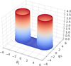Fig. 1 2D Gaussian shells likelihood. Radius r=2 and width w=0.1. Parameter boundaries are imposed as ±6. Likelihood values are coloured from blue (low) to red (high) to facilitate the visualisation of the figure.

4.1 n-d Gaussian shells

Sampling from an n-dimensional Gaussian shell is an analytically tractable problem widely used in the literature (Feroz & Hobson 2008; Speagle 2020). The likelihood contours are curved, thin, and nearly singular (see Fig. 1). Random-walk steps are inefficient, so this multimodal function stresses proposal geometry and temperature allocation. For n dimensions, radius r, width w, and peaks’ centres c_i, the likelihood is $$p(\theta )={\displaystyle \sum }_{i=1}^n\frac{1}{\sqrt{2\pi w^2}}\exp \left(-\frac{{\left(\left|\theta -c_i\right|-r\right)}^2}{2w^2}\right).$$(25)

This benchmark was used to assess the behaviour of the different samplers in efficiency and evidence estimation. reddemcee was set up with [16, 320, 640, 1] temperatures, walkers, sweeps, and steps, respectively, for a total of 3 276 800 samples. The adaptation hyper-parameters, τ₀, ν₀, were set as one tenth of the sweeps and one hundredth of the walkers, respectively. We adapted the temperature ladder during the first half of the sweeps, and then froze it. This entire adaptive phase was treated as burn-in: those samples were discarded before any statistical inference, but the time spent was included in the reported run-time (i.e. it affects the kenits metric). For comparison, the DNS runs were performed using dynesty (Speagle 2020) with its automated settings, testing three sampling modes: uniform, slice, and random-slice.

For dynesty, we calculated kenits using the reported number of likelihood calls, effectively measuring the sampling efficiency (fraction of independent samples) times all likelihood evaluations divided by the total run-time. For reddemcee, efficiency was defined as the inverse of the average autocorrelation time of the cold-chain, and kenits were computed as this efficiency multiplied by the number of likelihood evaluations (discarding burn-in samples, but not their run-time) over the full run-time. This method ensures a fair kenits comparison.

Sampler performance. All adaptive ladder methods are statistically similar (see Table 1); variance between ladder algorithms (0.04²) is smaller than the run-to-run variance of each method (≈0.12²), delivering ≈3.6–3.8 kenits. The best DNS method, dyn-rs, achieves 0.94±0.05 kenits, which is 26% of the APT average. This method also finishes the fastest, at 13.4s. It is worth mentioning that once converged, the efficiency does not radically change, so even by demanding a higher total iteration count as a stop condition, the kenits (and efficiency) would not dramatically increase. The dynamic algorithm stops at target precision, which, in the dyn-u case, required a much longer run-time with many more samples, whereas the slice methods finished faster with far fewer independent samples. In other words, there is a trade-off between thorough posterior sampling and evidence-estimation convergence speed. The same reasoning can be extended to MCMC, preserving much richer posterior information.

Evidence estimation. The proposed evidence estimation methods in Sect. 2.4 were tested and compared against the analytical value for the 2D case, ln 𝒵=−1.746 (see Table 2). The default TI method has ${{\Delta }_z|}_{\text{TI}}=8.394\%$, whereas the improved TI+ version achieves ${{\Delta }_z|}_{\text{TI+}}=0.324\%$ (an order of magnitude closer to the true value). The likelihood improves as well, with a ratio of exp(2.80 – 0.92) = 6.58. By contrast, the default SS has the highest $ℒ{(\stackrel{⌢}{{\rm Z}})|}_{\text{SS}}=4.326$ alongside a low ${{\Delta }_z|}_{\text{ss}}=0.117\%$. The SS+ counterpart shows slightly more conservative uncertainties (0.006 instead of 0.005) with $ℒ{(\stackrel{⌢}{{\rm Z}})|}_{\text{SS+}}=4.263$, and a slightly higher accuracy, ${{\Delta }_z|}_{\text{SS+}}=0.099\%$. The H+ method achieves the highest accuracy of all, ${{\Delta }_Z|}_{\text{H+}}=0.016\%$, along with a high likelihood, $ℒ{(\stackrel{⌢}{{\rm Z}})|}_{\text{H+}}=3.951$. Out of the DNS methods, dyn-u is the most reliable with ${{\Delta }_Z|}_{\text{dyn}-\text{u}}=1.751\%$, and a log-likelihood of $ℒ{(\stackrel{⌢}{{\rm Z}})|}_{\text{dyn}-\text{u}}=2.206$.

4.2 Gaussian egg-box

The Gaussian egg-box, dubbed after its likelihood shape (see Fig. 2), presents a periodic landscape with several equally high peaks, separated by deep troughs. It is an ideal stress test for mode completeness. Missing a single peak would render catastrophically wrong evidence. The likelihood function is $$p(\theta )={\left(2+{\displaystyle \prod }_{n=1}^{dim}\cos \left(\frac{\theta }{4}\right)\right)}^{{\overline{\beta }}_e},$$(26) where ${\overline{\beta }}_e=5$ was used, defining the narrowness of the peaks. The prior volume was limited to [0, 10π], and a fine grid integration gives ln 𝒵=235.856, which was used as the true value. We used the same set-up as in Sect. 4.1.

Sampler performance. For the ladder adaptation methods, the SAR and SMD methods rank best at 5.79 ± 0.29 and 5.66 ± 0.23 kenits with overlapping uncertainties, followed closely by the other methods (see Table 3). Out of the DNS methods, dyn-rs has the lowest wall-time as well as the highest kenits count, 0.82 ± 0.07, 14.2% of the SAR kenits.

Evidence estimation. As seen in Table 4, the TI algorithm misses the mark by Δ_𝒵=11.53%, with the worst overall likelihood: $ℒ(\stackrel{⌢}{{\rm Z}})=-0.643$. TI+ improves this to Δ_𝒵=1.43%, with a likelihood ratio of exp(2.658 − (−0.643)) = 26.87. The SS yields a log-likelihood of $ℒ(\stackrel{⌢}{{\rm Z}})=2.618$. Its SS+ counterpart marginally reduces Δ_𝒵 from 1.25% to 1.21%, with $ℒ(\stackrel{⌢}{{\rm Z}})=2.771$. The H+ method outperforms SS+ and TI+, achieving $ℒ(\stackrel{⌢}{{\rm Z}})=1.099$ and $ℒ(\stackrel{⌢}{{\rm Z}})=3.082$. Out of the DNS methods, dyn-u finds all modes (extremely accurate Δ_𝒵=0.201), albeit at the cost of many likelihood calls. Meanwhile, slice-based samplers are faster but slightly undersample some modes (evidence biases). dyn-u has the highest log-likelihood out of the DNS methods, at 1.828. Against H+, it gives a ratio of exp(3.082 – 1.828) = 3.5, which is almost four times as likely.

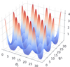Fig. 2 Gaussian egg-box likelihood, with 16 different modes. Likelihood values are coloured from blue (low) to red (high) to facilitate visualisation.

4.3 Hybrid Rosenbrock function

The Rosenbrock function is a long, thin, curved valley with strong non-linear correlations, slightly resembling a banana. The hybrid-Rosenbrock function is an extension that provides analytic evidence for any dimension (Pagani et al. 2019). Its likelihood is $$p(x)=-a{\left(x_1-\mu \right)}^2-{\displaystyle \sum }_{j=1}^{n_2}{\displaystyle \sum }_{i=2}^{n_1}{b}_{j,i}{\left(x_{j,i}-x_{j,i-1}^2\right)}^2,$$(27) where x _j,i, μ ∈ ℝ, and a, b_j,i ∈ ℝ⁺ are arbitrary constants. Its evidence is $$\mathcal{Z}=\sqrt{\frac{{\pi }^n}{a\cdot {{\displaystyle \prod }}^{\text{}}{b}_{j,i}}},$$(28) where n = (n₁ − 1) - n₂ + 1, and n₁ is the number of dimensions in each of the n₂ groups. Per Goodman & Weare (2010), a scale factor of 1/20 was chosen, with a = 1/20 and all b_j,i = 100/20, so the distribution is shaped like a narrow ridge, providing a challenging posterior shape (see Fig. 3).

To assess temperature evolution in the 2D case, the APT setup was changed to [24, 120, 1024, 1], increasing the number of temperatures to 24 and the sweeps to 1 024, while decreasing the walkers to 120, roughly maintaining the total iterations the same as in previous benchmarks.

Sampler performance. The SAR method ranks best with 14.65 ± 0.59 kenits, followed closely by SGG, GAO, and ETL. SMD ranks last, with 6.40 ± 0.41 kenits. For the DNS methods, dyn-rs ranks first with 0.77 ± 0.02 kenits, and dyn-u ranks last with 0.34 ± 0.02 kenits, and almost twice the wall-time (see Table 5). In this scenario, SAR presents increased kenits over dyn-rs by a factor of 19.03, almost 20 times more efficient at producing independent samples.

Evidence estimation. The H+ method relies completely on SS+, dropping TI+ segments (see Table 6). This can be attested by the poor TI+ performance compared to SS+. The slicesampling methods present negative log-likelihoods, indicating substantially underestimated errors.

A 3D case for the Rosenbrock function was also explored (results discussed in Section 6). Generally, the trends held, with reddemcee outperforming in sampling efficiency, and all ladder methods producing accurate evidences (see Table 11).

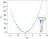Fig. 3 Probability contour of the 2D Rosenbrock function. The inset key shows how the colours relate to the probability.

5 Exoplanet detection from radial velocities

A real-world application of the APT ladder dynamics developed in Section 3 and evidence-estimation methods introduced in Section 2.4 is presented for the nearby G-dwarf HD 20794. Hosting at least three super-Earths whose RV semi-amplitudes are lower than 1 m s⁻¹, the system combines low amplitudes, multiplicity, and a long-period planet, all features that make model selection and evidence estimation particularly demanding. The innermost signals at 18 and 90 days were first identified in the HARPS discovery paper (Pepe et al. 2011), while subsequent analyses revealed an outer candidate with a period of ~650d that spends a significant fraction of its eccentric orbit inside the stellar habitable zone (Nari et al. 2025).

As such, this system provides an ideal test-bed for assessing the performance of our APT dynamics and evidence-estimation algorithms on a real-world example. The main features that make exoplanet RV fitting challenging are directly reflected in the previous benchmarks: the strong phase transition in C_ν is captured by the Gaussian shells, multi-modality and mode completeness in a many-alias situation (for a sparsely sampled period) in the Gaussian egg-box, and the curved, highly correlated ridges typically seen in the angular orbital parameters are emulated by the hybrid Rosenbrock function. In this section, the work by Nari et al. (2025) was followed, with us applying reddemcee to the combined HARPS+ESPRESSO time series, contrasting the resulting evidence with that reported in the literature.

5.1 Model and likelihood

Each exoplanet is characterised by five Keplerian parameters, P – the period, K – the semi-amplitude, e – the eccentricity, $\overline{\omega }$ – the longitude of periastron, and M₀ – the phase of periastron passage, $${\mathcal{K}}_j(t)=K_j\cdot \left[\cos \left(v_j\left(t,P_j,e_j,M_{0j}\right)+{\overline{\omega }}_j\right)+e_j\cos \left({\overline{\omega }}_j\right)\right],$$(29) where the subscript j indicates each exoplanet and ν_j is the true anomaly. In addition, each instrument is given an offset, γ (an additive constant), and a jitter, σ_INS (added in quadrature to the measurement error, corresponding to a white noise component). Therefore, under the assumption of Gaussian-like errors, the loglikelihood is $$\ln ℒ=-\frac{1}{2}{\displaystyle \sum }_{INS}{\displaystyle \sum }_i^{N_{INS}}\left(\frac{{\xi }_{i,\text{INS}}^2}{\left({\sigma }_i^2+{\sigma }_{\text{INS}}^2\right)}+\ln \left({\sigma }_i^2+{\sigma }_{\text{INS}}^2\right)\right)-\frac{N\ln (2\pi )}{2},$$(30) where the sub-indices i and INS correspond to the i-th RV measurement (taken at a time t_i) and to each instrument, respectively. The residuals, ξ_i,INS, are defined as the difference between the data and the model. Three distinct datasets plus three Keplerian signals add up to a total of 21 parameters or dimensions.

5.2 Parameter estimation and model selection

For an in-depth methodology follow-up, refer to Appendix B. The models compared are: (1) just white noise (H₀); (2) a single sinusoid (1S); (3) two sinusoids (2S); (4) three sinusoids (3S); (5) three Keplerians (3K); and (6) four Keplerians (4K). The sinusoidal models (S) treat planets as having circular orbits. The 3K model corresponds to the three confirmed planets, and 4K to the inclusion of an additional candidate.

For the evidence estimation (see Table 7), dyn-rs is consistent with SAR, up to the most complex models. For the 3S , 3K, and 4K models, they have a 4.6, 6.8, and 4.6 In $\stackrel{⌢}{{\rm Z}}$ difference, respectively. On the other hand, the SAR log-evidence is all within the reference values’ uncertainties except for the 1S case, which shows a moderate discrepancy (8.7). This could be due to random variation or differences in how noise was treated, but importantly the model ranking is unaffected.

Table 8 compares the estimated evidence errors to the actual run-to-run scatter (the ratio ${\widehat{\sigma }}_{\mathcal{Z},\text{estimated}}/{\widehat{\sigma }}_{\mathcal{Z},\text{empirical}}$). An ideal ratio is 1. Values ≪1 mean the method underestimates its true uncertainty, and ≫1 means overestimation. The dyn-rs ratios are all very low for complex models (0.04–0.12), severely underestimating the uncertainty with overly confident evidences, whereas reddemcee yields values much closer to unity (e.g., 0.63 for the 3K). Underestimation of error in multi-planet cases could lead to overconfident claims of detection; therefore, reddemcee (along the H+ estimator) provides more reliable uncertainties.

Performance-wise, APT achieves a higher kenits count in the simpler models, with a turnover point at 3K in favour of dyn-rs. This may be attributable to the modest fixed number of walkers (256) in the APT sampler (see Appendix B for details). In practice, one could adjust the walker count for efficiency’s sake, but it was kept constant for consistency between benchmarks.

For the parameter estimation, the two methods produce consistent results (see Table 9). Notably, the APT-derived parameter posteriors are slightly more asymmetrical and tighter (see K₂ and K₃). Also, the eccentricity estimates seem less averse to boundary solutions, as is seen in $e_1={0.057}_{-0.057}^{+0.045}$ and $e_2={0.026}_{-0.026}^{+0.007}$, both of which are consistent with e = 0.

6 Discussion

The evidence-estimation algorithms introduced in Section 2.4 have proven to be far more reliable than their unmodified counterparts. Furthermore, whether to apply the TI or the SS method is mostly problem-dependent, and the hybrid algorithm seems to be a good compromise when there is no a priori information about the problem at hand. Moreover, our proposed evidence estimators provide a solid, if not better, alternative to dedicated evidence-sampling methods. This is exemplified by the real-world case studied in Section 5.

Across the simplest problems we tested (few dimensions, nearly constant specific heat), all ladder strategies converge to an almost geometric ladder and yield a similar performance. Differences emerge as the problem’s complexity grows, and since a common problem astrophysicists face is that of dimensionality, we discuss it further next.

6.1 Increasing dimensionality

We took the Gaussian shells problem described in Sect. 4.1 and increased its dimensionality without modifying any hyperparameters, in order to demonstrate how the methods scale. As dimensionality grows, we see a very much expected efficiency decrease (see Table 10), as well as the SMD outperforming other methods. At 15 dimensions, it becomes the most effective, with a margin far exceeding the run-to-run scatter. In second place, GAO and ETL come tied (with overlapping confidence intervals), being around 14% slower, followed by the SAR – 19% slower – and the SGG – 34% slower. This supports the intuition that maximising swap distance is beneficial in high-dimensional spaces where local energy traps abound. On the other hand, dyn- rs, still the best DNS method, presents kenits at ~13% of the SMD average.

For evidence estimation, with the modest amount of temperatures proposed for this benchmark, the TI method degrades considerably, with a Δ_𝒵 of ~ 72% (see Table A.1). The TI+ soothes this, with Δ_𝒵 11.3%. Nevertheless, the error due the discretisation remains a problem in this benchmark. For the SS method, the evidence estimate is excellent (Δ_𝒵=2.56), with the highest $ℒ(\stackrel{⌢}{{\rm Z}})=2.1658$. The SS+ method presents a slight deterioration over its classic counterpart. The H+ presents a higher likelihood (and lower Δ_𝒵) than either TI+ or SS+.

By increasing the dimensionality of the Rosenbrock function to 3D, the evidence estimation results (H+) are best for ETL with $ℒ(\stackrel{⌢}{{\rm Z}})=2.901$, followed by SGG and GAO, with $ℒ(\stackrel{⌢}{{\rm Z}})=1.841$ and 1.561, respectively (see Table 11). The kenits values present a similar trend to that of the shells, with 2.98 (SAR), 2.50 (SMD), 3.46 (SGG), 3.03 (GAO), and 2.85 (ETL), and 0.02 (dyn-u), 0.55 (dyn-s), and 0.74 (dyn-rs).

6.2 Burn-in

How fast the adaptation optimally distributes the ladder depends on both the problem at hand and the adaptation hyper-parameters ν₀ and τ₀. We stress-tested adaptation by setting the 15D shells with 640 sweeps (as in Sect. 4.2 and Sect. 6.1) to use 320, 160, 64, and 32 sweeps as burn-in (see Table A.2). H+ is the method most resilient to an uncalibrated ladder. It is the only method that retains positive $ℒ(\stackrel{⌢}{{\rm Z}})$ values after the 25% burn-in, with values of In ${\stackrel{⌢}{Z}|}_{H+}=-24.939\pm 0.037$, –24.980±0.031, –24.984±0.034, and –24.996±0.041 for 50%, 25%, 10%, and 5%, respectively.

6.3 Ladder adaptation

For low-dimensional targets (2D shells, egg-box), every method settles on an almost geometric ladder, due to C_ν(β) being almost flat. As the dimensionality grows, C_ν develops a broad peak around the phase-transition region, and the objectives react differently. For example, the SAR spreads the temperatures uniformly in swap probability, and therefore stretches the ladder on both sides of the peak, while SMD concentrates the replicas where the specific heat is large, maximising the average information transfer, as is seen by its clear lead at 15D in Table 10.

Longer runs are realised for this scenario, 15D shells, with 10 000 sweeps instead of 640, to examine the convergence of the ladder adaptation. All schemes compress the first ~200 sweeps into a fast logistic-like relaxation of the temperature gaps, after which the diminishing adaptive factor, κ(t) (Eq. (14)), forces a slow power-law tail. In practice, almost the whole ladder shape is set in under 5% of the computational budget, supporting the choice of freezing the ladder after a user-defined burn-in.

Fig. 4 displays the ladder evolution of the SAR and SMD methods, respectively. A notable difference is that the SMD method has a layered swap rate, whereby the cold chain swaps frequently (0.7) and the hot chain seldom does (0.2), whereas the SAR keeps a steady swap rate of 0.5 for all temperatures.

Fig. 5 shows the final ladders as chain density (proportional to C_ν) as a function of temperature. The dashed vertical lines indicate where Δβ is smaller, as well as where the transition between TI and SS is applied in the hybrid method.

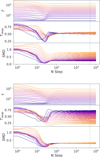Fig. 4 Temperature ladder evolution for the 15D Gaussian shells in the SAR regime (top) and SMD regime (bottom). In the x-axis is the current iteration. From top to bottom are the temperature ladder evolution, T, the swap acceptance ratio, Tswap, and the SMD. Colours represent each chain, where blue is the coldest (β=1), with temperature increasing towards the red, where the hottest chain is omitted. The vertical dashed black line indicates where the adaptation stops.

6.4 Number of temperatures

A natural question that arises is how many temperatures are enough. The answer, as one might expect, is that it depends. When doing an APT run, there are two objectives in mind: posterior and evidence estimation. More temperatures might be redundant posterior-wise, not contributing with additional information to the cold chain. At the same time, more temperatures provide a finer grid for the evidence estimation. Nonetheless, it is possible to dabble into this question, by analysing the temperature evolution of the ladder. If the mixing is low, increasing the temperatures will result in a more efficient run. This may be measured by comparing the additional chains computational cost against the efficiency (or kenits) increase. Visualising the likelihood variance as a function of temperature (the TI) can be helpful. A smoothly increasing curve will not be affected as much as a ladder-like curve by decreasing temperatures. This can also be appreciated by the Cν plot. A ladder-like behaviour would be seen as multiple sharp peaks (as in the HD 20794 3K model, see Fig. 6 with a secondary small peak at around β=0.4), whereas a smooth curve is seen as a single smooth peak (as in the 15D shells, see Fig. 5).

Another matter is how the different evidence-estimation algorithms proposed are affected. The 15D shells (with 10 000 sweeps) were re-run with N_β=6, 8, 12, and 16 (see Table A.3). The TI method by decreasing temperatures presents a linear fall-off with $\sqrt{{ℒ}_{\stackrel{⌢}{Z}}}$. This result can also be easily derived from Eq. (8), which reveals that the log-evidence error is proportional to $\frac{1}{\text{ntemps}}$. The TI+ method presents a huge improvement over TI, although still fails to reach the mark in temperature-poor regimes. The SS methods remain extremely accurate even at low N_β = 6, with Δ_𝒵=1.78 and $ℒ\left(\widehat{Z}\right)=2.02$. The geometrical bridge in SS+ yields a small accuracy gain (lower Δ_𝒵 for every N_β), while bringing a small drop in $ℒ\left(\widehat{Z}\right)$, due to the slight increase in the error estimate.

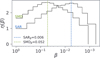Fig. 5 Chain density per temperature range for the SAR and SMD methods in the 15D Gaussian shells. The dashed blue line denotes the maximum of the SAR, with the green one representing the maximum of the SMD. Both lines also denote the regions where the TI or SS algorithms are applied in the hybrid method.

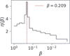Fig. 6 Chain density per temperature range for the HD 20794 3K SAR run. The vertical dashed red line marks the distribution maximum.

7 Conclusions

We have introduced reddemcee, an APT ensemble sampler that combines three next-level techniques – flexible ladder adaptation, robust evidence estimation, and practical error quantification – into a single, easy-to-deploy package. Three of the five ladder adaptation algorithms are new implementations from this work (SMD, SGG, ETL), reliable alternatives to the most commonly used SAR method, as is demonstrated in our benchmarks (see Section 4). All of these methods converge in a few sweeps and deliver cold-chain mixing efficiencies around an order of magnitude higher than DNS across our tests. In the challenging 15D Gaussian-shell benchmark, reddemcee sustained > 2 ken- its, about 7 times faster than the best DNS configuration, while the SMD ladder proved particularly resilient as dimensionality grew.

We devised three evidence estimators – two original implementations, TI+ and SS+, and a novel hybrid approach – that combine curvature-aware interpolation with bridge sampling. These estimators yield accurate log-evidence and maintain realistic uncertainties even when the number of temperatures is decreased beyond what is optimal.

A real-world application to the HD 20794 RV dataset shows that reddemcee reproduces literature model rankings, recovers planetary parameters with tighter – yet statistically consistent – credible intervals, and supplies evidence uncertainty that closely tracks run-to-run dispersion. Crucially, this performance was obtained without manual ladder tuning: the same hyperparameters were used from no-planet to four-planet models and from 6 to 21 dimensions.

Overall, reddemcee demonstrates that a carefully engineered APT sampler can match, and occasionally surpass, state- of-the-art DNS, both in sampling throughput and in evidence estimation, while retaining the posterior-inference strengths that make MCMC indispensable. Future work will explore on-the-fly convergence diagnostics, further widening the sampler’s applicability to the increasingly complex problems faced in modern astrophysics and beyond.

Acknowledgements

PAPR and JSJ gratefully acknowledge support by FONDE-CYT grant 1240738, from the ANID BASAL project FB210003, and from the CASSACA China-Chile Joint Research Fund through grant CCJRF2205. For the n-d Gaussian shells, Gaussian egg-box, and Rosenbrock function benchmarks parallelisation was not used and computing was limited to single-core for all algorithms. For the exoplanet detection benchmark, parallelisation was used with 24 threads. All the benchmarks were performed on a computer with an AMD Ryzen Threadripper 3990X 64-Core Processor with 128Gb of DDR4 3200Mhz RAM. We thank the anonymous referee for insightful suggestions that enhanced the quality of this manuscript. We are grateful to Fabo Feng and Mikko Tuomi for stimulating early discussions on planet detection. We would also like to thank Dan Foreman-Mackey for the excellent library emcee (Foreman-Mackey et al. 2013), which opened a most exciting new world. Typesetting was carried out in Overleaf (Digital Science UK Ltd. 2025).

References

Appendix A Gaussian shells

Appendix B HD 20794

Each dataset, HARPS03, HARPS15, and E19, is nightly binned, then sigma clipped (3σ), and measurements where the error is higher than 3 times the median error are excluded, leaving out 512, 231, and 63 RVs respectively, for a grand total of 806 RVs. Priors were matched to those stated by Nari et al. (2025), with unspecified priors left to an educated guess. For offset a prior ~𝒰(−3, 3) was chosen, and for jitter ~𝒩(0, 5), truncated at [0, 3]. For eccentricity e and longitude of periastron ω, we use the change of variable $$e_c=\sqrt{e}\cos (\omega );e_s=\sqrt{e}\sin (\omega ),$$(B.1) to linearise the circular parameter ω, improving sampler performance, as in Hou et al. (2012b). Point estimates and uncertainties for all parameters are defined as the posterior maxima and the corresponding 1-σ highest-density intervals (HDIs), rather than the more commonly used medians and corresponding 1-σ percentiles, reflecting our methodological preference for mode-based summaries.

Both methods had matching estimates for the H₀ model (with little variance). This value was chosen as offset for the reference values from the literature. We tried to follow the recipe of executing five runs and selecting the three with highest evidences. But this could not be applied to all models due to inconsistent results.

For the dynesty runs (random-slice sampling, 3 000 live- points), the 1S model consistently found P₁ = 18.314 d, K = 0.61 ms⁻¹, with In $\widehat{Z}=-1218.1\pm 2.7$, presenting a 46.1 difference against the H₀ model ln $\widehat{Z}=-1264.20\pm 0.04$. The 2S run (3 000 live-points) consistently added a signal with P₂ = 89.6 d and K₂ = 0.44 ms⁻¹ (signal subindex were shifted so P₁<P₂, and so on), with ln $\widehat{Z}=-1193.3\pm 2.4$, a difference of 24.9 against 1S.

An extra sinusoid brought multiple solutions in 3S at P₃ = 655, 1 018, and 1 426 d, the former being the solution with the highest maximum likelihood. The number of live-points was gradually increased until this solution was obtained at least three times out of five consecutive runs. At 5 000 live-points this solution was obtained consistently (5 out of 5 times), bringing an evidence difference of 24.2 with the 2S model.

Changing the sinusoids for Keplerians in the 3K model seems to eliminate this problem, since P₃ = 655 d appeared consistently amongst runs (3 000 live-points). For consistency, we also did the runs with increasing live-points, but when doing this the algorithm appears to get stuck in lower likelihood peaks more often. With 6 000 live-points we consistently got P₃ = 1 378 d, with an evidence 15 lower than P₃ = 655 d, and a maximum likelihood 20 lower. The increase in evidence compared to the 3S model (3.1) is tinier than both the reference value and the one obtained with the SAR method.

The 4K model did not converge to a single solution, obtaining 85.5 d, 111 d, 1011 d, or 1420 d as the fourth signal. The best evidence was obtained by the period P₄ = 85.54 d, while the best likelihood by P₄ = 111.23 d.

By comparing the differences between each model’s best solution, our dyn-rs results match the reference only for Δ_𝒵(H₀, S 1) and Δ_𝒵(S 1, S 2), with diverging results in increasing models by 5.3, 2.6, and −4.2, respectively. This could be explained by the high standard deviation (e.g., for the 4K, 4.6 in the reference and 3.8 in dyn-rs) or to sampler setup differences.

On the other hand, doing the same exercise against the SAR run provides much closer differences to the reference: 0.3, 2.2, −1.5, 1.6, and −0.2, with the highest values corresponding to Δ_𝒵(2S, 3S ) and Δ_𝒵(3S, 3K), and well within variance.

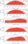Fig. B.1 HD 20794 posteriors for the first Keplerian in the 3K SAR run.

The reddemcee runs used 16 temperatures, 256 walkers, and 5 000 sweeps, increasing by 2 500 extra sweeps for each model, with 17 500 sweeps for the 4K, to facilitate the adaptation stationarity without ‘hand-tuning’ the adaptive parameters.

The 1S model consistently found the P = 18.314 d signal, with an evidence of ln $\widehat{Z}=-1217.1\pm 0.3$, and a difference of 47.9 with the H₀ model. Adding a signal found P₂ = 89.66 d consistently, with an evidence improvement of 23.5. The third sinusoid shifted this period slightly to 89.7 d, whilst adding one at P₃ = 652.2 d, and improving the evidence by 29.1. Changing the sinusoids to Keplerians brought an improvement of 5.2 evidence-wise, with eccentricities of e₁ = 0.057, e₂ = 0.026, e₃ = 0.467. The top of the posterior samples for the first Kep- lerian can be seen in Fig. B.1, with the last two parameters the aforementioned e_s and e_c in Eq. B.1. Additionally, Fig. B.2 (top) shows a corner plot (scatter plot matrix for multidimensional samples) for the same Keplerian, revealing parameter covariances: P₁ and K₁ have tight posteriors, with each off-diagonal panel being nearly circular. Both have a little correlation with eccentricity (denoted by their elongation over e_c, e_s). The centre of the e_c, e_s panel indicates a low value for eccentricity. The direction of its isotropic shape defines ω. The phase of periastron passage M₀ is coupled to the eccentricity vector, the textbook RV degeneracy. The third signal, with a higher well-defined eccentricity, does not present this degeneracy, as seen in Fig. B.2.

Finally, the 4K model brought both P₄~1440 d and ~111 d, with similar evidences and likelihoods.

The step decrease in kenits for the more complex model is attributed to the low walker count. It is also worth noting the difference in both consistency and wall-time in these models. For 3K and 4K the standard deviation in dyn-rs was 2.6 and 3.8 respectively, compared to 0.4 and 0.9 in reddemcee. Furthermore, the average wall-time in dyn-rs was 150.26±32.46, and 112.77±5.2 minutes, whereas in reddemcee it was 57.68±2.57, and 77.21±2.42 minutes. Time-wise, the runs were not only significantly shorter, but also more consistent.

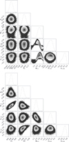Fig. B.2 HD 20794 corner plot for the first (top) and third (bottom) signals in the 3K model. Figures made with the corner package (Foreman-Mackey 2016).

Appendix C Evidence estimators

C.1 Geometric-bridge stepping stones

For the temperature ladder 1 = β₁ > … > β_B ≥ 0, at each β_i we have an ensemble of W walkers evolving over T sweeps. For each adjacent pair (β_i, β_i+1) and for every sweep, we build a symmetric BRIDGE (Meng & Wrong 1996; Gronau et al. 2017) between the two ensembles bridge (Meng & Wong 1996; Gronau et al. 2017) between the two ensembles $$\begin{array}{ll}\text{from}{\beta }_i\text{:\hspace{0.17em}}\hfill & A_{t,i}=\frac{1}{W}{\displaystyle \sum }_{w=1}^W\ln {ℒ}^{\text{Δ}{\beta }_i/2},\hfill \\ \text{and\hspace{0.17em}from}{\beta }_{i+1}\text{:}\hfill & C_{t,i}=\frac{1}{W}{\displaystyle \sum }_{w=1}^W\ln {ℒ}^{-\text{Δ}{\beta }_i/2}.\hfill \end{array}$$(C.1)

If the ladder is still adapting, we use the per-sweep Δβ_i,t, otherwise (as in this manuscript) a single averaged Δβ_i. Then we average over sweeps to get ${\mu }_{A,i}=\overline{A_{t,i}}$ and ${\mu }_{C,i}=\overline{C_{t,i}}$. Each ratio $\frac{{\mu }_{A,i}}{{\mu }_{C,i}}$ estimates r_i via the geometric bridge. Multiplying all these ratios, or adding their logs, gives the log-evidence estimate $$\ln {\widehat{\mathcal{Z}}}_{SS+}={\displaystyle \sum }_{i=1}^{B-1}\left(\ln {\mu }_{A,i}-\ln {\mu }_{C,i}\right).$$(C.2)

For the sampling error $\widehat{\sigma }\stackrel{2}{s}$ we treat the per-sweep vectors [A_t; | C_t;] as a correlated time series across sweeps, estimating the long-run covariance with multivariate OBM, and use the delta method for $g\left(\mu \right)={\Sigma }_i\left(\ln {\mu }_{A,i}-\ln {\mu }_{C,i}\right)$ to get $\text{Var}\left[\widehat{Z}\right]=\widehat{\sigma }\stackrel{2}{s}$ (Flegal & Jones 2008; Wang et al. 2018). This method effectively steps along the ladder with a geometric bridge at each step, propagating an autocorrelation-aware uncertainty.

C.2 Piecewise interpolated thermodynamic integration

For each sweep t = 1,…, T, we take the per-temperature mean log-likelihood ${\overline{\ell }}_{i,t}=\frac{1}{W}{\Sigma }_{w=1}^W\ln {ℒ}^{{\beta }_i,t}$. Now, for each sweep we interpolate the curve ${\text{E}}_{\beta }\left[U\right]\left(\beta \right)$ with PCHIP (Fritsch & Butland 1984), and integrate, resulting in a series ${\widehat{Z}}_t$. The time-average of this series is the evidence estimate $$\ln {\widehat{\mathcal{Z}}}_{\text{TI}+}={\displaystyle \sum }_{t=1}^T{\widehat{z}}_t.$$(C.3)

To estimate ${\widehat{\sigma }}_D$ we form a coarser ladder by dropping every other β, recompute the same PCHIP integral to get ${\widehat{Z}}_t^{\left(2\right)}$, timeaverage to In ${\widehat{Z}}_{\text{TI}+}^{\left(2\right)}$, and set $${\widehat{\sigma }}_D=\ln {\widehat{Z}}_{\text{TI}+}^{(2)}-\ln {\widehat{Z}}_{\text{TI}+}.$$(C.4)

To estimate ${\widehat{\sigma }}_S$, if the ladder is no longer adapting, we treat ${\widehat{Z}}_t$ as a correlated univariate time series over the sweeps, estimate its long-run covariance ς with OBM, and set $\widehat{\sigma }\stackrel{2}{s}=\frac{\Sigma }{T}$. Otherwise, with a ladder still adapting (under diminishing adaptation), with N_β the length of the interpolated values, we take the per-sweep trapezoid TI block as $$\begin{array}{cc}{\widehat{z}}_t={\displaystyle \sum }_{i=1}^{N_{\beta }}\text{Δ}{\beta }_{i,t}\cdot S_{i,t},& S_{i,t}=\frac{\left({\overline{\ell }}_{i,t}+{\overline{\ell }}_{i+1,t}\right)}{2}.\end{array}$$(C.5)

With the S_t series, we estimate the multivariate long-run covariance ς_s with multivariate OBM, and propagate with mean widths $\overline{d\beta }=\Delta {\beta }_t$: $${\widehat{\sigma }}_D^2=\text{Var}\left[{\widehat{z}}_t\right]={\overline{d\beta }}^{\top }{\text{Σ}}_S\overline{d\beta }.$$(C.6)

Note that for the total error, since ${\widehat{\sigma }}_D$ and ${\widehat{\sigma }}_S$ are added in quadrature, they are being treated as independent. For the adaptative case, we need a stationary adaptation settled in the ladder, which should happen under diminishing adaptations after some sweeps have passed, depending on the hyper-parameters on κ(t) (see Eq. 14).

All Tables

All Figures

	Fig. 1 2D Gaussian shells likelihood. Radius r=2 and width w=0.1. Parameter boundaries are imposed as ±6. Likelihood values are coloured from blue (low) to red (high) to facilitate the visualisation of the figure.
In the text

	Fig. 2 Gaussian egg-box likelihood, with 16 different modes. Likelihood values are coloured from blue (low) to red (high) to facilitate visualisation.
In the text

	Fig. 3 Probability contour of the 2D Rosenbrock function. The inset key shows how the colours relate to the probability.
In the text

Fig. 4 Temperature ladder evolution for the 15D Gaussian shells in the SAR regime (top) and SMD regime (bottom). In the x-axis is the current iteration. From top to bottom are the temperature ladder evolution, T, the swap acceptance ratio, Tswap, and the SMD. Colours represent each chain, where blue is the coldest (β=1), with temperature increasing towards the red, where the hottest chain is omitted. The vertical dashed black line indicates where the adaptation stops.

In the text

	Fig. 5 Chain density per temperature range for the SAR and SMD methods in the 15D Gaussian shells. The dashed blue line denotes the maximum of the SAR, with the green one representing the maximum of the SMD. Both lines also denote the regions where the TI or SS algorithms are applied in the hybrid method.
In the text

	Fig. 6 Chain density per temperature range for the HD 20794 3K SAR run. The vertical dashed red line marks the distribution maximum.
In the text

	Fig. B.1 HD 20794 posteriors for the first Keplerian in the 3K SAR run.
In the text

	Fig. B.2 HD 20794 corner plot for the first (top) and third (bottom) signals in the 3K model. Figures made with the corner package (Foreman-Mackey 2016).
In the text

References

- Diamond-Lowe, H., Charbonneau, D., Malik, M., Kempton, E. M. R., & Beletsky, Y. 2020, AJ, 160, 188 [NASA ADS] [CrossRef] [Google Scholar]
- Digital Science UK Ltd. 2025, Overleaf [Google Scholar]
- Drummond, A., Nicholls, G., Rodrigo, A., & Solomon, W. 2002, Genetics, 161, 1307 [Google Scholar]
- Earl, D. J., & Deem, M. W. 2005, Phys. Chem. Chem. Phys. (Incorp. Faraday Trans.), 7, 3910 [Google Scholar]
- Feroz, F., & Hobson, M. P. 2008, MNRAS, 384, 449 [NASA ADS] [CrossRef] [Google Scholar]
- Feroz, F., Balan, S. T., & Hobson, M. P. 2011, MNRAS, 415, 3462 [Google Scholar]
- Flegal, J. M., & Jones, G. L. 2008, arXiv e-prints [arXiv:0811.1729] [Google Scholar]
- Ford, E. B., Lystad, V., & Rasio, F. A. 2005, Nature, 434, 873 [NASA ADS] [CrossRef] [Google Scholar]
- Foreman-Mackey, D. 2016, J. Open Source Softw., 1, 24 [Google Scholar]
- Foreman-Mackey, D., Hogg, D. W., Lang, D., & Goodman, J. 2013, PASP, 125, 306 [Google Scholar]
- Fritsch, F. N., & Butland, J. 1984, SIAM J. Sci. Statist. Comput., 5, 300 [Google Scholar]
- Gelman, A., & Meng, X.-L. 1998, Statist. Sci., 13, 163 [Google Scholar]
- Gelman, A., Carlin, J. B., Stern, H. S., & Rubin, D. B. 2004, Bayesian Data Analysis, 2nd edn. (Chapman and Hall/CRC) [Google Scholar]
- Gilks, W. R., Roberts, G. O., & Sahu, S.K. 1998, J. Am. Statist. Assoc., 93, 1045 [Google Scholar]
- Goggans, P. M., & Chi, Y. 2004, in American Institute of Physics Conference Series, 707, Bayesian Inference and Maximum Entropy Methods in Science and Engineering, eds. G. J. Erickson, & Y. Zhai, 59 [Google Scholar]
- Gonzalez, G. 1997, MNRAS, 285, 403 [Google Scholar]
- Goodman, J., & Weare, J. 2010, Commun. App. Math. Comput. Sci., 5, 65 [NASA ADS] [CrossRef] [Google Scholar]
- Gregory, P. C. 2005, ApJ, 631, 1198 [NASA ADS] [CrossRef] [Google Scholar]
- Gronau, Q. F., Sarafoglou, A., Matzke, D., et al. 2017, J. Math. Psychol., 81, 80 [Google Scholar]
- Hansmann, U. H. E. 1997, Chem. Phys. Lett., 281, 140 [Google Scholar]
- Higson, E., Handley, W., Hobson, M., & Lasenby, A. 2019, Statist. Comput., 29, 891 [Google Scholar]
- Hou, F., Goodman, J., Hogg, D. W., Weare, J., & Schwab, C. 2012a, ApJ, 745, 198 [NASA ADS] [CrossRef] [Google Scholar]
- Hou, F., Goodman, J., Hogg, D. W., Weare, J., & Schwab, C. 2012b, ApJ, 745, 198 [NASA ADS] [CrossRef] [Google Scholar]
- Jenkins, J. S., Díaz, M. R., Kurtovic, N. T., et al. 2020, Nat. Astron., 4, 1148 [Google Scholar]
- Katzgraber, H. G., Trebst, S., Huse, D. A., & Troyer, M. 2006, J. Statist. Mech. Theory Exp., 2006, 03018 [Google Scholar]
- Kofke, D. 2002, jcph, 117, 6911 [Google Scholar]
- Kone, A., & Kofke, D. 2005, J. Chem. Phys., 122, 206101 [Google Scholar]
- Lartillot, N., & Philippe, H. 2006, Syst. Biol., 55, 195 [Google Scholar]
- Marcy, G. W., & Butler, R. P. 2000, PASP, 112, 137 [Google Scholar]
- Maturana-Russel, P., Meyer, R., Veitch, J., & Christensen, N. 2019, Phys. Rev. D, 99, 084006 [Google Scholar]
- Mayor, M., & Queloz, D. 1995, Nature, 378, 355 [Google Scholar]
- Meng, X.-L., & Wong, W. 1996, Statist. Sin., 6, 831 [Google Scholar]
- Miasojedow, B., Moulines, E., & Vihola, M. 2013, J. Computat. Graph. Statist., 22, 649 [Google Scholar]
- Nari, N., Dumusque, X., Hara, N. C., et al. 2025, A&A, 693, A297 [NASA ADS] [CrossRef] [EDP Sciences] [Google Scholar]
- Oaks, J. R., Cobb, K. A., Minin, V. N., & Leaché, A. D. 2018, arXiv e-prints [arXiv:1805.04072] [Google Scholar]
- Pagani, F., Wiegand, M., & Nadarajah, S. 2019, arXiv e-prints [arXiv:1903.09556] [Google Scholar]
- Pepe, F., Lovis, C., Ségransan, D., et al. 2011, A&A, 534, A58 [CrossRef] [EDP Sciences] [Google Scholar]
- Predescu, C., Predescu, M., & Ciobanu, C. V. 2004, J. Chem. Phys., 120, 4119 [Google Scholar]
- Rannala, B., & Yang, Z. 1996, J. Mol. Evol., 43, 304 [Google Scholar]
- Rathore, N., Chopra, M., & de Pablo, J. 2005, J. Chem. Phys., 122, 024111 [Google Scholar]
- Roberts, G., & Rosenthal, J. 2007, J. Appl. Probab., 44 [Google Scholar]
- Shenfeld, D. K., Xu, H., Eastwood, M. P., Dror, R. O., & Shaw, D. E. 2009, Phys. Rev. E, 80, 046705 [Google Scholar]
- Skilling, J. 2004, in American Institute of Physics Conference Series, 735, Bayesian Inference and Maximum Entropy Methods in Science and Engineering, eds. R. Fischer, R. Preuss, & U. V. Toussaint, 395 [Google Scholar]
- Speagle, J. S. 2020, MNRAS, 493, 3132 [Google Scholar]
- Sugita, Y., & Okamoto, Y. 1999, Chem. Phys. Lett., 314, 141 [Google Scholar]
- Swendsen, R. H., & Wang, J.-S. 1986, Phys. Rev. Lett., 57, 2607 [CrossRef] [MathSciNet] [PubMed] [Google Scholar]
- van der Sluys, M., Raymond, V., Mandel, I., et al. 2008, Class. Quant. Grav., 25, 184011 [Google Scholar]
- Veitch, J., Raymond, V., Farr, B., et al. 2015, Phys. Rev. D, 91, 042003 [NASA ADS] [CrossRef] [Google Scholar]
- Vines, J. I., Jenkins, J. S., Berdiñas, Z., et al. 2023, MNRAS, 518, 2627 [Google Scholar]
- Vousden, W. D., Farr, W. M., & Mandel, I. 2016, MNRAS, 455, 1919 [NASA ADS] [CrossRef] [Google Scholar]
- Wang, Y.-B., Chen, M.-H., Kuo, L., & Lewis, P. O. 2018, Bayesian Anal., 13, 311 [Google Scholar]
- Xie, W., Lewis, P., Fan, Y., Kuo, L., & Chen, M.-H. 2011, Syst. Biol., 60, 150 [Google Scholar]