| Issue |
A&A
Volume 706, February 2026
|
|
|---|---|---|
| Article Number | A145 | |
| Number of page(s) | 13 | |
| Section | Astrophysical processes | |
| DOI | https://doi.org/10.1051/0004-6361/202556805 | |
| Published online | 06 February 2026 | |
Afterglow linear polarization signatures from steep GRB jets: Implications for orphan afterglows
1
Astrophysics Research Center of the Open University (ARCO), The Open University of Israel P.O. Box 808 Ra’anana 4353701, Israel
2
Department of Natural Sciences, The Open University of Israel P.O. Box 808 Ra’anana 4353701, Israel
3
Department of Physics, The George Washington University Washington DC 20052, USA
★ Corresponding author: This email address is being protected from spambots. You need JavaScript enabled to view it.
Received:
10
August
2025
Accepted:
30
November
2025
Abstract
Gamma-ray bursts (GRBs) are the strongest explosions in the Universe, and are powered by initially ultra-relativistic jets. The angular profile of GRB jets encodes important information about their launching and propagation near the central source, and can be probed through their afterglow emission. Detailed analysis of the multiwavelength afterglow light curves of recent GRBs shows evidence of an extended angular structure beyond the jet’s narrow core. The afterglow emission is determined by the jet angular structure, our viewing angle, and the magnetic field structure behind the shock, often leading to degeneracies when considering the light curves and broadband spectrum alone. Such degeneracies can be lifted with joint modeling of the afterglow light curves and polarization. In this work we studied the evolution of the afterglow linear polarization and flux density from steep core-dominated GRB jets, where most of their energy resides within a narrow core. We explored the dependence of the light and polarization curves on the viewing angle, jet angular energy structure, and magnetic field configuration and provide an analytical approximation for the peak polarization level, which occurs at a time close to that of a break in the light curve. Finally, we demonstrated how our results can be used to determine the nature of orphan GRB afterglows, distinguishing between a quasi-spherical dirty fireball and a steep jet viewed far off-axis, and applied them to the orphan afterglow candidate AT2021lfa detected by the Zwicky Transient Facility (ZTF).
Key words: polarization / relativistic processes / shock waves / gamma-ray burst: general / stars: jets
© The Authors 2026
 Open Access article, published by EDP Sciences, under the terms of the Creative Commons Attribution License (https://creativecommons.org/licenses/by/4.0), which permits unrestricted use, distribution, and reproduction in any medium, provided the original work is properly cited.
This article is published in open access under the Subscribe to Open model. This email address is being protected from spambots. You need JavaScript enabled to view it. to support open access publication.
1. Introduction
Gamma-ray bursts (GRBs) are violent astrophysical events associated with the launch of relativistic jets, that originate in newly born accreting compact objects (Eichler et al. 1988; MacFadyen & Woosley 1999). Such systems are not spherically symmetrical, and the brief prompt γ-ray emission can be observed only when the observer is located within, or very close to, the jet opening angle (e.g., Beniamini & Nakar 2019). GRBs are followed up with long-lasting emission, termed the afterglow. This multiwavelength component is associated with the formation of a relativistic shock, due to the interaction of the relativistic outflow with the ambient medium. The shock accelerates charged particles that radiate linearly polarized synchrotron radiation under the influence of shock-generated magnetic fields (e.g., Paczynski & Rhoads 1993; Katz 1994; Katz & Piran 1997; Waxman 1997a,b; Sari et al. 1998; Mészáros et al. 1998; Gruzinov & Waxman 1999; Ghisellini & Lazzati 1999; Sari 1999). Earlier works on GRBs assumed the jet has a simple top-hat angular structure, in which the energy and Lorentz factor are uniform within a narrow core opening angle and drop sharply beyond it. Such a structure was shown to explain the appearance of achromatic steepenings in the afterglow light curve, caused by the deceleration of the flow and the Lorentz factor reaching a value comparable to the inverse of half of the core opening angle. Following this stage, there are no new areas of the jet that are revealed to the observer as it decelerates, leading to a geometrical jet break in the afterglow light curve (Rhoads 1997, 1999; Sari et al. 1999). However, a detailed afterglow light curve analysis of recent events shows evidence for the existence of an extended angular structure of the jet beyond its core, most notably, GW 170817 (Gill & Granot 2018; Lazzati et al. 2018; Mooley et al. 2018; Ghirlanda et al. 2019; Gill et al. 2019; Troja et al. 2019; Govreen-Segal & Nakar 2023). In some cases, different jet structures may reproduce the same multiwavelength light curves, making the jet structure difficult to constrain based on light curve fits alone. In the case of GRB 221009A, the multiwavelength afterglow light curves can be reproduced with two different jet structures (O’Connor et al. 2023; Gill & Granot 2023). In Birenbaum et al. (2024), we show that while the existing polarization limits on the X-ray and optical afterglow (Negro et al. 2023) agree with both models, an earlier measurement could have differentiated between the models, making this observable a unique tool for probing the angular structure of the jet.
Numerical simulations suggest that the jet develops an extended angular structure during its propagation within the progenitor system (Gill et al. 2019; Gottlieb et al. 2021; Govreen-Segal & Nakar 2024), which can be merger ejecta in the case of a short GRB (Eichler et al. 1988; Narayan et al. 1992; Berger et al. 2013; Tanvir et al. 2013; Abbott et al. 2017; Mooley et al. 2018) or a stellar envelope in the case of a long GRB (MacFadyen & Woosley 1999; Galama et al. 1998; Woosley & Bloom 2006; Metzger et al. 2011). Such a structure can also develop within a dynamical time even if a top-hat jet is initially injected (Granot et al. 2001; Zhang & MacFadyen 2009; Gill et al. 2019; Govreen-Segal & Nakar 2024). The structure that emerges reflects the processes the jet underwent before breaking out, as well as the jet’s production conditions, making the jet structure an important quantity to constrain. Steep jets, which hold most of the energy within the jet core, can be formed when the jet is weakly magnetized, which acts to reduce the amount of mixing between the light jet material with that of the heavy confining medium via suppression of hydrodynamical instabilities (Gottlieb et al. 2020; Beniamini et al. 2020). Such a structure can also be consistent with most afterglow observations (Granot & Kumar 2003; Beniamini et al. 2020; O’Connor et al. 2023; Gill & Granot 2023).
In recent years, optical transients with afterglow-like temporal evolution and no associated GRBs have been detected using the Zwicky Transient Facility (ZTF). The origin of these events is under debate (Lipunov et al. 2022; Ho et al. 2022; Li et al. 2025). At the time of writing, 12 such events have been found using ZTF, 6 of which without a retroactively associated prompt γ-ray counterpart (with confirmed redshift; Ho et al. 2020, 2022; Andreoni et al. 2021; Perley et al. 2025; Srinivasaragavan et al. 2025). One of these events, AT2021lfa, is detected in optical, radio, and X-ray. The optical light curve features clearly rising flux which peaks and then declines as a power law. While the declining phase of the transient was initially captured by ZTF, the preceding rising phase was serendipitously found in archival MASTER-OAFA data (Lipunov et al. 2021, 2022). A comparison of the optical light curve with known on-axis GRB afterglow light curves, conducted by Lipunov et al. (2022), shows similarities which motivate this transient’s relation to GRBs. The authors fit top-hat jet optical afterglow models to the light curve and vary the viewing angle, resulting in the on-axis model fitting the data better than the off-axis model, as it produces a rising phase that is too steep to fit the MASTER-OAFA data1. They concluded that this orphan afterglow candidate is the result of a dirty fireball with baryon-contaminated ejecta that fails to produce a GRB. However, the off-axis afterglow scenario the authors fit does not include the possibility of a steep structured jet, which can also exhibit a slow rise in flux, a peak, and a power-law decline in time (Granot et al. 2002; Kumar & Granot 2003; Nakar 2020; Gill & Granot 2020; Beniamini et al. 2022). This possibility was considered in recent work that revisits the multiwavelength observations of AT2021lfa and manages to fit the optical light curve with both on-axis jet and off-axis jet models using the afterglowpy tool (Ryan et al. 2020; Li et al. 2025). In their work, Li et al. (2025) show that an on-axis top-hat jet and an on-axis Gaussian jet both reproduce the optical light curve within the dirty fireball model framework. The off-axis structured jet scenario manages to reproduce the same light curve with either power-law or Gaussian jets.
While the light curves of these events fail to pinpoint the exact geometry of the system and whether it is on- or off-axis, such events are expected to differ greatly in polarized light (Granot et al. 2002; Rossi et al. 2004; Gill & Granot 2020; Teboul & Shaviv 2021; Birenbaum et al. 2024). In addition, the detection of linear polarization can confirm the synchrotron source of the emission (e.g., Gruzinov & Waxman 1999; Ghisellini & Lazzati 1999; Sari 1999). Measuring this quantity along with the light curve in the optical can indicate whether the system originates in a dirty fireball or in a structured off-axis jet.
In this paper we characterize the polarization signature from steep jets, starting with structure dependence of on- and off-axis jets and then expanding the off-axis jet analysis to viewing angle effects and the impact of the magnetic field structure behind the shock on the observed polarization and flux. Building on the conclusions drawn from these models, we offer an analytical approximation for the dependence of the polarization peak on the geometrical parameters of the system. Finally, we demonstrate the ability of polarization modeling and measurements in discerning between dirty fireballs and off-axis structured jets on the orphan afterglow candidate AT2021lfa, extending the work done by Li et al. (2025) to the polarized regime.
2. Methods
The calculations presented in this work follow the formulas presented in the methods section of Birenbaum et al. (2024, B24 hereafter). The basic model assumed in B24 and this work features a 2D axisymmetric relativistic shock propagating into a cold ambient medium with a power-law rest-mass density profile ρ ∝ R−k. Following Gill & Granot (2018), the jet dynamics are assumed to be locally spherical (neglecting lateral dynamics) and the emission is calculated from a 2D surface associated with the afterglow shock front. The jet angular profile is expressed in terms of the distribution of the isotropic equivalent kinetic energy and initial Lorentz factor, which are described by Ek, iso = EcΘ−a (with a > 2 corresponding to a steep jet, see Fig. 1) and Γ0 − 1 = (Γc − 1)Θ−b where Θ = [1 + (θ/θc)2]1/2. The subscript c denotes properties of the jet core. The shock surface is divided into angular cells around the jet symmetry axis, defined by θ. The emitting region right behind the shock radiates synchrotron emission under the influence of a shock generated magnetic field whose comoving direction  and corresponding magnitude B′ in each cell are drawn from a probability distribution set by the magnetic field stretching factor ξ (for a more detailed explanation, see Appendices A and B of B24).
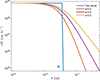 |
Fig. 1. Jet angular energy structures considered in this work with core opening angle θc = 2°. The top-hat jet model (blue lines) acts as a step function in energy. The other models behave according to the power-law jet model with varying steep slopes with a > 2 (see Sect. 2 and B24). |
Following these initial calculations, we proceed to calculate the Stokes parameters Iν, Qν, Uν from each cell and integrate over their contributions in order to evaluate the overall observed linear polarization and flux. Full details of the calculation are presented in B24.
3. Results
As shown in B24 and Rossi et al. (2004), the angular structure of the jet has a profound impact on the polarization signature of GRB afterglows. The shallow jet case (a < 2) was studied in detail in B24. Here we extend and complete that study by exploring the parameter regime of steep jets (a > 2), which are often referred to as core-dominated jets, since most of their energy resides in their narrow cores. In this work the same afterglow parameters chosen in B24 are selected so that the observed frequency does not cross any of the critical synchrotron frequencies (see Table 1). In the sections below, results are shown for both on-axis jets, viewed from within their core opening angle (with normalized viewing angles q ≡ θobs/θc < 1) and off-axis jets, (with q > 1). The cases considered in this section are set with a uniform initial Lorentz factor profile (b = 0).
3.1. Viewing angle and jet structure
3.1.1. Jets viewed on-axis (0 < q < 1)
We start by exploring the polarization and light curves of steep jets from on-axis systems, set with q ≡ θobs/θc = 0.7. This parameter regime is explored within the context of the power-law jet structure, described in Eqs. (2)–(4) of B24 (see Fig. 1). In Fig. 2, we present the polarization curves (upper panel) and light curves (lower panel) for models with a constant normalized viewing angle q = 0.7, magnetic field structure that is random within the plane of the shock (ξ → 0) and varying angular steep jet structures (a > 2).
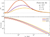 |
Fig. 2. Observed polarization degree (upper panel) and flux (lower panel) as a function of time for the power-law jet model at observed frequency ν = 1015 Hz (PLS G) with a flat initial Lorentz factor distribution (b = 0) and a random magnetic field structure, confined to the shock plane (ξ → 0). The various values of a represent different slopes for the power-law jet wings. The observer is located at q = 0.7. |
The polarization curves of the various angular energy structures all exhibit a single polarization peak and no rotation of the polarization angle (polarization degree remains positive throughout). Such behavior of the observed polarization differs from that of top-hat jets and broken power-law jets, which feature a 90° rotation of the polarization angle that is manifested in our formalism as a change in the sign of the polarization degree (Sari 1999; Ghisellini & Lazzati 1999; Granot & Konigl 2003; Rossi et al. 2004; Shimoda & Toma 2021; Birenbaum & Bromberg 2021; Lan et al. 2023; B24). This new behavior of on-axis jets stems from the use of the power-law jet model, which features a smooth transition between the jet core and the extend jet structure and can eliminate the polarization angle rotation altogether. This important feature will be studied in detail in future work (Birenbaum et al. in prep.).
While the shape of the polarization curve remains similar, its magnitude varies and grows as the structure becomes steeper with growing values of a. This happens due to increased asymmetry in the visible part of the emitting region as the contribution of the jet core dominates the polarized emission with less contribution from the extended jet structure.
The light curves of these models, varying only by the power-law index of the jet angular energy profile, show similar shapes while varying slightly in terms of magnitude, where shallower structures, with lower values of a, feature higher observed flux as they contain more energy. While the light curves are similar to one another, each structure has its own unique polarization signature, and with sufficient measurements and careful modeling, the jet structure can be determined.
3.1.2. Jets viewed off-axis (q ≥ 1)
In this section, we describe the polarization signature of steep jets (a > 2) viewed off-axis (q ≥ 1). This setup is studied using the smooth power-law jet configuration, as it provides a smooth transition between the jet core and its extended structure (i.e., power-law wings, see Fig. 1).
We start by exploring the dependence of the light and polarization curves on the angular energy profile of the jet by varying the value of a, and setting the normalized viewing angle to be constant with q = 5 (see left panel of Fig. 3). The magnetic field structure behind the shock is set to be random in the plane of the shock with ξ → 0. The case of a misaligned top-hat jet is shown in blue solid lines for comparison purposes. Similarly to the behavior shown in Sect. 3.1.1, the height of the polarization peak increases with the steepness of the jet, encapsulated by rising values of a. We also note that the polarization peak is associated with a break in the light curve, similar to the behavior seen in shallow jets and on-axis steep jets (see B24 and Fig. 2). As emission from the core starts to reach the observer, asymmetry in the visible region reaches its peak and so does the polarization. Following the revelation of the most energetic part of the jet to the observer, the light curve experiences a steepening. This effect is purely geometrical and is therefore largely achromatic2.
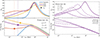 |
Fig. 3. Observed polarization degree (upper panels) and flux (lower panels) at observer frequency ν = 1015 Hz (PLS G) with a flat distribution of initial Lorentz factor (b = 0) and a random magnetic field structure confined to the face of the shock (ξ → 0) for off-axis jets. The direction of the polarization vector remains constant throughout the temporal evolution. Left panel: The viewing angle is set to be constant for an off-axis jet with q = 5 with varying values of a. The polarization degree reduces with a and its peak coincides with a light curve break. We mark with a star and vertical dashed lines the time of a light curve dip, expected when the emission transitions from angular structure dominated to core dominated in the Blandford-Mckee deceleration regime (Beniamini et al. 2020). At this time, the onset of a plateau phase can be seen in the polarization curve. Right panel: The jet structure is held constant with a = 3.5 while the off-axis viewing angle changes. As the observer line of sight approaches the jet symmetry axis with reducing values of q, the polarization peak becomes lower and occurs at earlier times. |
The height of the polarization peak for the shallowest structure considered in this work with a = 2.5 (left panel of Fig. 3, yellow solid curves) is the lowest one. This corresponds to the conclusion drawn in B24 and in Sect. 3.1.1 that shallower jets produce lower levels of polarization due to increased levels of symmetry around the line of sight. The polarization peak of the steepest structure considered in this work, with a = 5.5 (left panel of Fig. 3, red solid curves) converges to the polarization peak of the top-hat jet structure (solid blue curves) at the same misalignment, indicating maximum asymmetry has been reached. This point is explored in more detail in Sect. 3.3.
In Beniamini et al. (2020), light curves from off-axis steep jets have been explored in detail with the aim of characterizing them using light curve features alone. These light curves exhibit one or two peaks depending on the viewing angle and jet structure. For light curves that feature two peaks, the earliest one is associated with the end of the coasting phase near our line of sight, where Γ is constant until enough mass from the outer medium accumulates to start decelerating the blast wave. This deceleration time occurs early in the evolution of the system and is not seen in the light curves presented in this current work. The second light curve peak can be seen in all light curves presented in this section and is attributed to the geometrical effect induced by the jet core coming into view. In cases where the system geometry causes these times to be well separated, there is an additional light curve feature in the shape of a light curve dip, occurring at an observer time tdip which separates the end of the coasting phase from the onset of the angular structure dominated phase. During the latter phase, the observed emission originates from a region at an angle  off the line of sight3, toward the jet core. Since the emission is dominated by the jet structure, the observed flux gradually rises as more energetic regions start contributing. The transition time tdip is found at the intersection point of two power-law curves fitted to the light curve, marked with a star and a vertical dotted line in the left panel of Fig. 3. This critical time manifests as the onset of a plateau in the polarization curve, seen most clearly in the steeper structures (in red and purple solid lines). The power-law energy structure probed at this time range causes a self-similar behavior of the emission region, resulting in constant polarization degrees which hold up to the point the observed flux switches to becoming core-dominated. This behavior becomes less pronounced in the other setups explored in this work (corresponding to smaller values of a) as they present smaller dynamical range in time and do not allow enough temporal separation between tdip and the second light curve break, tb. Moreover, for smaller a values, the effective core of the jet becomes larger (see Fig. 1), allowing emission from it to reach an observer at a specific viewing angle at an earlier time compared to a steeper structure. This acts to reduce the time difference between tdip and tb and almost erase the polarization plateau seen in the a = 5.5 case.
Another geometrical parameter that affects the observed flux and its corresponding polarization curve is the viewing angle. Its effect is demonstrated in the right panel of Fig. 3, where the upper panel corresponds to the polarization curve and the lower panel shows the light curves. The magnetic field structure is set to be random in the plane of the shock (ξ → 0) with a steep angular energy structure (a = 3.5). The normalized viewing angle is set to be off-axis with values of q ≥ 1 which differ by line texture. One notable feature is the change in the height of the polarization peak, which increases with growing values of q. As the observer becomes more misaligned with the jet symmetry axis the level of asymmetry in the system increases, which leads to higher levels of polarization. At the most extreme misalignment degree in our study (q = 5, solid purple curve), the height of the polarization peak starts approaching the maximal polarization level of synchrotron radiation (e.g., Rybicki & Lightman 1979; Granot 2003; B24). As discussed for the previous plot, it can be seen that the polarization peak is associated with a break in the light curve, due to dominant contribution to the observed flux from jet core emission, which becomes visible around this time. This correlation, as well as the dependence of the polarization peak height on the normalized viewing angle, is explored in detail in Sect. 3.3. The time at which the polarization peaks4 changes with the viewing angle, as it is dominated by the angular proximity of the line of sight to the jet core. The closer the observer line of sight is to the jet symmetry axis, the earlier the observed flux will be dominated by the jet core, leading to an earlier break in the light curve and a peak in the polarization curve, which correspondingly occurs at a higher flux level. A similar trend can also be seen for shallow jets (B24).
3.2. Magnetic field 3D orientation
Up until this point we investigated the effects of the geometrical parameters (the jet energy profile power-law index, a, and normalized viewing angle, q) on the observed flux and consequent polarization of GRB afterglows that involve steep jets, while assuming a random magnetic field in the plane of the shock (set with ξ → 0). The effect of the magnetic field structure on the observed polarization and light curves is studied in this section by setting the viewing angle and jet angular energy structure as constants (with q = 3 and a = 3.5 respectively) and varying the structure of the magnetic field behind the shock with the value of ξ. The generally random magnetic field corresponds to an isotropic field (in 3D) that is stretched in the radial direction (along the local shock normal) by a factor of ξ (following Sari 1999; Gill & Granot 2020, B24), such that ξ → 0 corresponds to a random field completely in the plane of the shock while ξ → ∞ corresponds to an ordered field in the radial direction (for details, see B24). The polarization degree of each curve does not change sign during its temporal evolution since the viewing angle is off-axis.
We consider five representative values of the magnetic field stretching factor ξ and calculate their corresponding polarization (Fig. 4, upper panel) and light curves (Fig. 4, lower panel), which are presented in shades varying from purple to gray in Fig. 4. The choice of modeled stretching parameters includes two extreme values (ξ → 0, ∞), the limits imposed by the radio afterglow polarization of GW 170817 (ξ = 0.75, 1.15; Gill & Granot (2018), B24) and one intermediate value with ξ > 1 as suggested by Arimoto et al. (2024). It is apparent from the upper panel of Fig. 4 that the polarization changes sign, indicating a 90° rotation of the polarization vector, as the stretching factor ξ crosses 1. This is caused by a change in the dominant component of the magnetic field behind the shock, from predominantly in the plane of the shock (ξ < 1) to predominantly radial (ξ > 1).
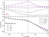 |
Fig. 4. Observed polarization degree (upper panel) and flux (lower panel) at observer frequency ν = 1015 Hz (PLS G) with a flat distribution of initial Lorentz factor (b = 0), smooth power law energy profile with a = 3.5, observed with q = 3. The structure of the magnetic field changes with the value of ξ. The direction of the polarization vector changes by 90° once the stretching factor ξ crosses 1, manifesting as a change in the sign of the polarization degree. The polarization peak happens at about the same time for all curves and is close to the break time of the light curve. |
For the two extreme values of the ξ parameter, which correspond to the extreme magnetic field configurations: purely random field in the plane of the shock (ξ → 0) and radial magnetic field (ξ → ∞), we see high values of polarization at times close to a break in the light curve. Although the polarization degree does peak for the ξ parameters of order unity, the height of the peak is lower due to the mixing of the two field components, such that the local polarization contributions of their emission largely cancel out, leading to low polarization. In the case of a completely isotropic magnetic field with ξ = 1, the polarization degree would be 0 throughout.
As the value of ξ grows, the polarization degree starts to exhibit a different behavior at post-peak times, where instead of reducing to zero, it asymptotes to a constant value. This can be seen in Fig. 4 in the case of ξ → ∞ (dashed gray lines), the polarization remains constant following the break in the light curve and its asymptotic value approaches the maximum level of polarization of synchrotron radiation, Πmax, marked by a horizontal crimson dashed line (Rybicki & Lightman 1979). In addition, the corresponding light curve exhibits a steeper decline post break compared to lower values of ξ. A similar high-ξ behavior is not seen when shallow jets are considered (B24). This change in asymptotic behavior can be understood through the jet structure.
For steep jets that feature a high value of ξ and are observed off-axis, the emitting region in late times is dominated by the narrow jet core. Combined with the radially dominated magnetic field, associated with high values of ξ, the core behaves as a point source of synchrotron radiation with an almost uniform magnetic field, which emits highly polarized radiation (Rybicki & Lightman 1979), leading to a constant level of polarization at these times. In the limit θobs ≪ 1 ≪ Γc(tobs), the comoving angle of the emitted photons that reach the observer relative to the radial direction, θ′=arccosμ′, is given by
 (1)
(1)
Following the break in the light curve, at times tobs > tb, the Lorentz factor in the core obeys Γc(tobs) < 1/θobs, such that θ′≪1,  and θ′≈2θobsΓc(tobs)∝Γc(tobs)∝t−αΓ. The comoving specific emissivity scales as j′ν′ ∝ (ν′)−α[sin ψ′]ϵ where ϵ = 1 + α for optically thin emission from an electron distribution that is isotropic in the comoving frame (Granot 2003)5, and ψ′ is the pitch angle of the emitting electron, which in our case is ψ′=θ′. Therefore, the flux density temporal decay index steepens by Δαt = αΓ(1 + α) relative to the ξ → 0 case. For PLS G, the temporal spectral index is
  while for a uniform external medium neglecting lateral spreading
  , which leads to
  for p = 2.5, close to the difference in slopes we get from our semi-analytical calculation. For
  this steeper decay lasts until the nonrelativistic transition time when Γc(tobs)∼1 and θ′∼θ = θobs. For
  this steeper decay lasts until θ′∼ξ−1 ⇔ Γc(tobs)∼(ξθobs)−1, i.e., up to tobs ∼ tbξ1/αt, at which point the nonradial field starts dominating the emitted flux that reaches the observer and the regular flux decay rate is resumed.
3.3. Behavior of peak polarization
In Sections 3.1.1, 3.1.2 and 3.2 we showed how the afterglow light and polarization curves change as the viewing angle, jet angular energy structure and magnetic field structure behind the shock vary. In addition, we highlighted the evident connections between these two observables.
Following previous work (Sari 1999; Granot 2003; Granot & Konigl 2003; Rossi et al. 2004; Birenbaum & Bromberg 2021; B24), we highlight in the upper panel of Fig. 5 the connection between the time the polarization level peaks (tPmax) and the time a geometrical break appears in the light curve (tb). The magnetic field structure is assumed to be random in the plane of the shock with ξ → 0. For slightly misaligned jets, viewed from within their core opening angle, the polarization peaks when a narrow region of the polarized ring, upon which the polarization vector is ordered, dominates the observed emission. Following this time, the light curve experiences a steepening as the whole core has been revealed to the observer and there are no more energetic new parts of the jet that contribute to the emission.
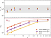 |
Fig. 5. Upper panel: Ratio of the polarization peak times tPmax to light curve break times tb as a function of normalized viewing angle q = θobs/θc for all steep jet structures considered in this work. We can see that these two times are within a factor of three from each other. Lower panel: Maximum polarization degree Pmax as a function of the normalized viewing angle q = θobs/θc. The maximum polarization level shows an almost linear rising trend for small values of q (solid lines), which correspond to systems viewed from within their effective core opening angle θc,eff. This trends flattens out at larger values of q (dotted lines) when the system is viewed off-axis with respect to the effective core. The size of this effective core grows as the jet becomes shallower, marking a change in the value of q where this turnover occurs, qc,eff. |
The off-axis structured jet scenario behaves similarly, where polarization peaks as the core is revealed to the observer and the light curve shows a break when the emission turns core-dominated. In the upper panel of Fig. 5, the ratio between the two times tPmax/tb is plotted as a function of the normalized viewing angle q and these two times are shown to be within a factor of 3 of one another (shaded gray region). This fortifies the relation between the two times and is consistent with the results shown in B24.
In the bottom panel of Fig. 5 we show the dependence of the peak polarization level Pmax on the normalized viewing angle q = θobs/θc for the steep jet structures considered in this work. As described in section 3.1.2, Pmax rises as the viewing angle grows due to increased asymmetry. In B24 we quantify this dependence using a simple toy model which uses a top-hat jet and find the functional behavior changes when the system is viewed on- or off-axis. For q < 1, the polarization level rises as ∝q1.1 while for q > 1 the behavior saturates into an asymptotic value. The general behavior of the polarization peak as function of q can be described as  where the value of χ is set by
 (2)
(2)
While this behavior holds for top-hat jets (see B24), it is strongly affected by the effective core size θc,eff, determined by the jet structure. This modified behavior can be seen for shallow jets (a ≤ 2), where the jet’s effective core angle becomes larger due to contributions from the energetic power-law wings, causing systems viewed off-axis to behave as if they are on-axis. These systems exhibit a rising trend in peak polarization levels that behaves as q1.1 (see B24) lasting up to a larger value of q before Pmax saturates. In the bottom panel of Fig. 5 we see that the turnover value of q at which the behavior switches becomes closer to 1 as the jet becomes steeper, indicating the effective core angle θc,eff is becoming smaller with less contribution from the jet power-law wings. We leave the exact definition of the effective core angle for future work.
In Fig. 6 we show the correlation between the peak polarization level and the power-law index of the angular energy structure, Pmax(a), for viewing angles in the range 0.7 ≤ q ≤ 5. The range of a-values shown here expands upon the results presented in B24 and covers the parameter space of both shallow and steep jets (0.5 ≤ a ≤ 5.5). We observe a different behavior with a for on- and off-axis viewing angles. For on-axis observers with q < 1, the peak polarization level rises as a power-law ∝a1.3. This trend can be explained by the increase in the asymmetry in the system as the value of a increases and the jet becomes steeper6. During the time of the peak in steeper jets, the observed flux is dominated by the energetic jet core, with a decreasing contribution from the jet power-law wings as the jet becomes steeper, which raises asymmetry in the system and its consequent polarization. This rising behavior changes for off-axis observers with q > 1 where it can now be described with a broken power law7 that rises as a1.4 and saturates to an asymptotic value of ∼0.63 at a turnover value acrit(q) that depends on the viewing angle. This asymptotic behavior is a result of the system approaching the maximum polarization level possible for a random magnetic field configuration that is confined to the shock plane (ξ → 0). We can describe the q > 1 dependence with the following expression
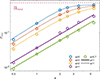 |
Fig. 6. Maximal polarization levels, Pmax, as a function of the power-law index of the energy angular profile, a, for various viewing angles and random magnetic field in the plane of the shock (ξ → 0). Values of a ≤ 2 and a > 2 correspond to shallow and steep jets, respectively. While jets observed from within their core opening angle θc (q < 1, solid lines) exhibit a power-law trend, Pmax ∝ a1.3, jets observed off-axis (q > 1, dotted lines) show a broken power-law behavior, which rises as ∝a1.4 before asymptotically approaching a constant level of polarization. The value of acrit where the turnover occurs depends on q due to the impact of the jet structure on its effective core size θc,eff. |
![Mathematical equation: $$ \begin{aligned} {P_{\max }}(a,q,\xi \!\rightarrow \!0) = 0.63\left[\left(\frac{a}{a_{\text{crit}}(q)}\right)^{-s(q)}+1\right]^{-1.4/s(q)}. \end{aligned} $$](/articles/aa/full_html/2026/02/aa56805-25/aa56805-25-eq15.gif) (3)
(3)
Here the turnover value is best fit with a power law acrit(q) = 4.84 ⋅ q−0.43 and the smoothness parameter of the break has been fitted with the expression s(q) = 1.14 ⋅ q0.87.
Finally, we analytically study how the peak polarization degree Pmax changes with the value of the magnetic field structure parameter behind the shock, by fixing the jet structure (a) and viewing angle (q) and changing the value of the stretching factor ξ from →0 (random magnetic field in the plane of the shock), through intermediate values, to →∞ (radial magnetic field). In Fig. 7 we present Pmax(ξ) for several configurations of the system (combinations of a and q). We find that Pmax approaches a constant value for each setup when the magnetic field is dominated by either the random (ξ ≪ 1) or radial (ξ ≫ 1) components. However, when these two components become comparable (ξ ∼ 1), the degree of cancellations in the system rises and reduces the observed polarization as a result. We mark in gray shaded area the limits on the magnetic field structure parameter imposed by upper limits on the polarization of the radio afterglow of GW 170817, derived by Gill & Granot (2018)8 and adapted to the terms of our model. This measurement points to a rather isotropic magnetic field behind the shock, which will produce low levels of polarization during the peak regardless of jet structure and viewing angle (see inset of Fig. 7). When the magnetic field is completely isotropic in all 3D directions, the polarization completely vanishes. This is evident in Fig. 7, with all curves crossing zero at ξ = 1. The asymptotic polarization level of the most asymmetric geometric setup we explore in this part (with a = 5.5 and q = 5 in solid red lines) has polarization levels that approach the maximum level of polarization for synchrotron radiation, Πmax (crimson dashed line), when ξ → ∞. This is achieved since in this regime the emission during the polarization peak is dominated by the narrow jet core and viewed off axis, with a uniform radial magnetic field that is misdirected w.r.t the line of sight. The change in Pmax with the value of ξ has been fitted with a hyperbolic tangent function of the form (B24):
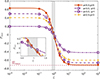 |
Fig. 7. Maximal polarization degree Pmax as a function of the magnetic field stretching factor ξ, in which synchrotron radiation is emitted. This relation is plotted for four combinations of the jet energy angular profile power-law index a and normalized viewing angle q, and is well described by a hyperbolic tangent of log10ξ for all values. The region of ξ imposed by the upper limits on the polarization of GW 170817 (0.75 < ξ < 1.15; Gill & Granot 2018, 2020; B24) is marked in shaded gray. The inset shows a zoomed-in image of this region. All curves change sign at ξ = 1. Detailed models can be found in Table A.1. |
 (4)
(4)
Here (A − D) and −(A + D) are the asymptotic values of Pmax at ξ → 0 and ξ → ∞, respectively; B is the width of the transition region; and C = tanh−1(D/A) ensures that Pmax(ξ = 1) = 0 as expected in a case of a completely isotropic magnetic field with ξ = 1. The fitted expressions for the models shown in Fig. 7 are presented in Table A.1 in Appendix A, where a slight dependence of A, B, C and D on a and q can be seen.
All the descriptions for the functional dependence of the peak polarization level on the magnetic field structure (through the stretching factor ξ), normalized viewing angle (q) and angular energy structure (through the power-law index a) can be combined into a single expression. This expression provides an approximation for the peak polarization level given the system’s geometrical conditions for values of ξ ≲ 1. This expression is of the following general form
![Mathematical equation: $$ \begin{aligned} {P_{\max }}=\Psi (a,q)\left[A\tanh (-B\log _{10}\xi +C)-D\right] , \end{aligned} $$](/articles/aa/full_html/2026/02/aa56805-25/aa56805-25-eq17.gif) (5)
(5)
where the values of A, B, C, and D can be found in Table A.1 and the functional dependence on q and a is given by
![Mathematical equation: $$ \begin{aligned} \Psi (a,q) = {\left\{ \begin{array}{ll} q^{1.1}\left(\frac{a}{3.5}\right)^{1.3}&q < 1 \;,\\ \left[\left(\frac{a}{a_{\text{ crit}}(q)}\right)^{-s(q)}+1\right]^{-1.4/s(q)}\frac{\sin 2\chi }{2\chi }&q>1 \;, \end{array}\right.} \end{aligned} $$](/articles/aa/full_html/2026/02/aa56805-25/aa56805-25-eq18.gif) (6)
(6)
with  and the q < 1 normalization on Ψ(q, a) is chosen according to the choice for the functional dependence on ξ from Table A.1. We can plug in the expressions in Table A.1 to get an analytical approximation for the peak polarization level as function of system parameters. Since in this work we find different behaviors for jets viewed on- and off-axis, below we give two different suggestions that approximate the peak polarization levels of steep jets. The expression for on-axis jets with q < 1, a > 2 and ξ ≲ 1:
![Mathematical equation: $$ \begin{aligned} {P_{\max }}= q^{1.1}\left(\frac{a}{3.5}\right)^{1.3}\left[0.31\tanh \!\left(0.38-2.1\log _{10}\xi \right)-0.11\right]\,. \end{aligned} $$](/articles/aa/full_html/2026/02/aa56805-25/aa56805-25-eq20.gif) (7)
(7)
For off-axis viewing angles, with q > 1, a > 2 and ξ ≲ 1, we obtain
![Mathematical equation: $$ \begin{aligned} {P_{\max }}= \Psi (a,q)\left[0.67\tanh \!\left(0.054-2.2\log _{10}\xi \right)-0.042\right]. \end{aligned} $$](/articles/aa/full_html/2026/02/aa56805-25/aa56805-25-eq21.gif) (8)
(8)
To re-normalize these expressions for other choices of the electron particle population power-law index p9, which denotes the value of Πmax, one can divide them by the value of Πmax and multiply by the corresponding value that fits the choice of p. The expressions presented in Eqs. (5)–(8) allow us to approximate the peak polarization level using the geometrical parameters of the system. Such expressions can be used when optical afterglow polarization is observed close to the light curve break time10 to constrain the geometrical properties of the system alongside modeling of the light curve, without the need for running complex models.
4. AT2021lfa: Orphan afterglow candidate
Afterglow model parameters for the dirty fireball and off-axis structured jet models of the R-band flux observations of AT2021lfa.
The optical transient AT2021lfa was first detected by ZTF at 05:34:48 UTC 2021 May 4. Followup observations found a power-law like flux decay, with no preceding detections and a source redshift of z = 1.063 (Yao et al. 2021a,b). Three hours before the first ZTF detection, the MASTER-OAFA robotic telescope recorded the same transient during a routine sky survey, showing a rising trend in observed flux (Lipunov et al. 2021, 2022). This transient has also been detected in radio, however the observations are suspected to heavily suffer from interstellar scintillation (Li et al. 2025). Comparison between the R-band light curve and other optical afterglows shows similarities which hint at a relation between this optical transient and GRBs (Lipunov et al. 2022). Additional Swift-XRT observations demonstrate a typical photon index that can be related to GRBs as well as brightness that is similar that of X-ray afterglows. Using correlations between the X-ray flux and prompt γ-ray brightness, Lipunov et al. (2022) deduce that if indeed this transient is related to a GRB, its prompt γ-ray emission should have been observed. However, searches in the archives of space γ-ray observatories did not yield a counterpart.
Afterglow-like transients that lack an associated prompt γ-ray emission are termed orphan afterglow candidates. If these transients are indeed related to GRBs, the lack of observed prompt γ-ray counterpart can be attributed to one of three reasons (Rhoads 2003; Huang et al. 2002; Lipunov et al. 2022; Li et al. 2025):
-
The GRB system was observed beyond the relativistic jet core, causing the prompt emission that comes from the jet core to be missed (while outflow along our line of sight is not relativistic enough to efficiently produce γ-rays, see Beniamini & Nakar 2019). A rising phase in the afterglow light curve can be attributed to emission from matter in the jet wings along our line of sight (Gill & Granot 2018; Beniamini et al. 2020). Such systems are termed in this work as off-axis structured jets.
-
The jetted matter did not reach a high enough Lorentz factor to efficiently produce prompt γ-ray emission due to baryon entrainment in the ejecta, which slows it down. In this scenario, our line of sight can be within the jet’s core. Although such a system will not produce a prompt γ-ray signal, it can produce an observable afterglow. We refer to such systems as dirty fireballs.
-
The prompt γ-ray emission was not observed due to incomplete sky coverage.
It is difficult to observationally distinguish between the different scenarios for orphan afterglows, whose prompt emission was not detected for intrinsic physical reasons (1 and 2 above). Huang et al. (2002) and Rhoads (2003) discuss ways to distinguish between the different scenarios based on their light curve evolution, as well as testing the long-term radio evolution.
The light curve analysis approach is taken by Lipunov et al. (2022) and the authors fit the optical light curve with a top-hat jet, viewed on- and off-axis. The authors conclude that if AT2021lfa is indeed an orphan afterglow, it must be the result of a dirty fireball, as the on-axis scenario manages to reproduce the rising phase of the optical light curve better than the off-axis one. They estimate an initial Lorentz factor of ∼20. The same approach is taken by Li et al. (2025) and the authors use the afterglowpy tool, which also takes into account the possibility of a structured jet, and use it to fit different models to the light curve. They find that the optical light curve is consistent with both the dirty fireball and the off-axis structured jet scenarios. The radio observations greatly suffer from interstellar scintillation, making them hard to model. While such an approach is exciting, it also emphasizes that light curve modeling alone sometimes cannot distinguish between different scenarios for orphan afterglow candidates.
In addition to the methods mentioned above (Huang et al. 2002; Rhoads 2003), Granot et al. (2002) suggested that polarization measurements should be included in orphan afterglow searches in order to constrain the GRB jet opening angle distribution. Here we follow these suggestions and demonstrate how strategically measured linear optical polarization can assist in discerning between the two intrinsic scenarios for the lack of observed prompt γ-ray emission for orphan afterglows. Our main result is presented in Fig. 8, in which we present afterglow models that follow the trends seen in the observed R-band light curve of AT2021lfa and show vastly different polarization signatures.
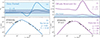 |
Fig. 8. Upper panels: Observed polarization curves corresponding to the dirty fireball (panel (a)) and off-axis structured jet (panel (c)) models for the R-band (optical) light curve of AT2021lfa. Polarization curves are presented for two values for the magnetic field stretching factor ξ: a random magnetic field confined to the plane of the shock (ξ → 0) and the more realistic ξ = 0.75, which also has a slightly weaker radial component. The ξ → 0 models exhibit higher polarization than the ξ = 0.75 models. The peak levels of polarization of the dirty fireball scenario are marked with blue (for ξ → 0) and dark blue (for ξ = 0.75) shading, for comparison with the off-axis structured jet scenario. Lower panels: Observed R-band flux for AT2021lfa (black data points, taken from MASTER-OAFA and ZTF; Lipunov et al. 2021, 2022; Yao et al. 2021b), and computed light curves according to the dirty fireball (panel (b), solid blue lines) and off-axis structured jet (panel (d), solid purple lines). Both models are able to describe the trends seen in the flux observations, while having very different geometrical parameters. Detailed afterglow parameters can be found in Table 2. |
The dirty fireball scenario for the R-band observations of AT2021lfa is presented in the left hand side of Fig. 8. Panel (b) shows the light curve, based on an adapted version of the fitted top-hat jet model of Li et al. (2025). The details of the afterglow model parameters are presented in Table 2. The main features of the model are its low initial Lorentz factor (Γc = 11.48) that does not enable prompt γ-ray production and emission, which means it won’t be observed even though the system is on-axis with q = 0.46 (Huang et al. 2002; Rhoads 2003). While the main features of the Li et al. (2025) dirty fireball model were kept in our analysis (system geometry and initial Lorentz factor), some adaptations were made to the afterglow model to account for flux normalization differences between our code and the afterglowpy tool. At early times, the modeled light curve shows a rising trend, which is meant to explain the MASTER observations. This trend corresponds to the pre-deceleration phase of the light curve, at which the flow coasts at a constant Γ = Γ0, culminating in a deceleration peak, as the dynamical solution transitions to the Blandford-Mckee deceleration phase (Blandford & McKee 1976; Gill & Granot 2018). Following this deceleration time, the light curve shows a declining power-law evolution that follows the trend of the observations, with a slight steepening at ∼2 days that corresponds to the jet break.
Panel (a) of Fig. 8 shows the corresponding polarization curves for two values of the magnetic field stretching factor: ξ → 0, which represents a purely random magnetic field in the plane of the shock, and the more realistic ξ = 0.75 (in blue and dark blue solid lines, respectively). In the pre-deceleration phase, the observed polarization degree for both models remains constant with a value →0. Since the flow is coasting at constant velocity, the initial angular scale of the emitting region on the shock face does not change with time (1/Γ0), which leads to constant observed polarization levels11. As the dynamical solution changes from coasting to Blandford-Mckee following the deceleration peak, edge effects begin to affect the observed region and the polarization signature of a top-hat jet, observed on-axis, appears. This temporal evolution is composed of two polarization peaks at opposing signs which correspond to a 90° difference in the polarization angle. In the slow cooling regime, where νm < νobs < νc, the afterglow image is limb-brightened (Sari 1997; Granot & Loeb 2001; Granot 2008) and may be approximated as a bright ring around the line of sight with an angular radius of 1/Γ upon which the polarization vector is radially oriented for ξ < 1 (Sari 1999; Granot & Konigl 2003; Nava et al. 2016; Shimoda & Toma 2021; Birenbaum & Bromberg 2021). When this ring is fully visible, the observed polarization is zero as cancellations across the ring are maximal in this symmetric system. However, as the shock decelerates, the visible region grows and eventually parts of the emitting ring disappear beyond the sharp jet edge, making the observed system less symmetrical around the line of sight. The first polarization peak occurs when a quarter of the ring is beyond the jet edge, which leads to negative polarization values, opposite in sign to the polarization values seen in previous section. When only half of the polarized ring remains visible, the polarization vanishes (as there is an instantaneous full cancellation) and then reappears rotated by 90°. The polarization degree reaches its second peak, with positive values, close to the jet break time as only a quarter of the polarized ring dominates the observed region (see Birenbaum & Bromberg 2021 for a visualization of this evolution). While the polarization signature is similar, its magnitude changes according to the structure of the magnetic field behind the shock. The random magnetic field structure, confined to the plane of the shock (ξ → 0, blue solid line) demonstrates polarization levels that reach 10% at peak (shaded blue region), while the more realistic value of ξ = 0.75, with a sub-dominant but comparable radial component, shows peak polarization level of ∼2.5% (shaded dark blue region).
The off-axis structured jet scenario is shown in the right part of Fig. 8 where panel (d) shows the observed R-band flux and a corresponding light curve, while panel (c) shows the polarization curves for two values of the magnetic field stretching factor: ξ → 0, and ξ = 0.75 (in purple and light purple solid lines, respectively). The main features of this model are a high initial Lorentz factor at the core (Γc = 390) that, when combined with a large off-axis viewing angle (q = 5.33), can explain the absence of an observed prompt γ-ray emission component. A steep angular structure beyond the jet core, in both energy (a = 2.5) and initial Lorentz factor (b = 3.2), allows for a shallower rise in flux that better explains the observed R-band flux at early times (Beniamini et al. 2020; Teboul & Shaviv 2021; Li et al. 2025). In the absence of spectral information, this model was constructed based on the observational optical features of AT2021lfa using the closure relations from Nakar et al. (2002) and Beniamini et al. (2020).
In the off-axis structured jet scenario, the rise in optical flux is attributed to the angular structure dominated phase (see explanation in Sect. 3.1.2 and in Beniamini et al. 2020). The light curve features a flat, prolonged peak due to an additional spectral crossing of νc by the observed frequency νobs during the geometrical peak time. The declining observed flux is attributed to the core-dominated phase, where the most energetic part of the jet has already been unveiled and is decelerating (see Sect. 3.1.2 and Beniamini et al. 2020). The matching polarization curves show an almost constant polarization degree during the rising phase of the light curve, as the flux is dominated by the power-law wings of the energy distribution, with a corresponding power-law brightness distribution, resulting in a self-similar behavior in terms of polarization. The level of polarization is determined by the combination of the offset from the jet symmetry axis and outflow geometry (i.e., jet angular structure), and for off-axis observers it can reach moderate to high levels, depending on the magnetic field structure (see Fig. 4 and related explanations in Sect. 3.1.2). As the observed emission turns core-dominated, the polarization levels begin to rise, culminating in a peak whose height depends on the geometrical parameters of the system (see Sect. 3.3). The polarization degree remains at a constant sign due to the off-axis orientation of the observer (see Sect. 3.1.2 and B24).
Comparison between the left and right panels of Fig. 8 demonstrates the potential of polarization measurements for differentiating between the dirty fireball and off-axis structured jet scenarios for orphan afterglow candidates. When we consider the same magnetic field structure behind the shock for the two scenarios, stark differences arise between the dirty fireball and off-axis structured jet models in the polarized regime. For both values of the magnetic field structure parameter ξ, there’s a factor 5 − 6 difference in polarization peak height. For ξ → 0, the off-axis structured jet model reaches a polarization peak of 57% close to the onset of the declining phase of the light curve while the dirty fireball model peaks later with a polarization peak height of 10%. Similar differences can be seen when considering the more realistic value of ξ = 0.75 with 11% and 2.5% respectively.
It is also evident that the off-axis structured jet model polarization remains above that of the dirty fireball at all times when considering the same value for the ξ parameter for both models. Another feature that can be seen in the dirty fireball polarization curves (due to the assumption of a top-hat jet) is the presence of a 90° rotation of the polarization angle, shown as a sign change of the polarization level. Such a feature is not seen in the polarization curve of the off-axis structured jet model and can possibly be another distinguishing factor between these two models.
While comparison between models that assume the same magnetic field structure behind the shock shows clear differences between the possible interpretations for orphan afterglows, one must remember that this parameter is still not well constrained by observations and it is not clear whether it varies between bursts. This can complicate the interpretation of sparse polarization measurements for orphan afterglows. For example, if we compare the polarization levels of the off-axis structured jet scenario with ξ = 0.75 (Fig. 8, light purple solid lines) and those of the dirty fireball model with ξ → 0 (Fig. 8 , blue solid lines), measured about 2–3 days after T0, we obtain similar levels of polarization from both models (∼10%). However, given that extreme values of ξ ≪ 1 or ξ ≫ 1 can be safely ruled out by current afterglow observations (Granot & Konigl 2003; Gill & Granot 2018, 2020; Stringer & Lazzati 2020), measuring Ptot ≈ 10% would strongly favor an off-axis jet model over a dirty fireball model.
The results shown in this section clearly demonstrate the potential benefit of strategically measuring polarization for orphan afterglow candidates. Not only can such detection confirm the synchrotron source of the emission (e.g., Gruzinov & Waxman 1999; Ghisellini & Lazzati 1999; Sari 1999), but combining this with detailed light curve modeling can shed light on the intrinsic reason the prompt γ-ray emission was not observed.
5. Discussion and conclusions
In this work we explored the polarization signature of afterglows from steep GRB jets and its relation to the observed flux density. We demonstrated how the measured afterglow polarization, alongside detailed modeling of its light curve, can provide crucial information regarding the jet structure, which is shaped by the processes the jet underwent before breaking out of its confining medium. This geometrical information can be crucial when trying to decipher the origin of orphan afterglow candidates. While light curve-based models can be degenerate, we showed that the expected polarization can differ, providing motivation to measure polarization for such events.
Using the semi-analytical tool developed in B24, which assumes an axisymmetric 2D shock, we focused on power-law jet structures and expanded the results to the regime where most of the energy is concentrated in the narrow jet core. Such models are motivated by both numerical simulations of GRB jets breaking out of their confining media and by observations of recent GRBs. We find that for a fixed viewing angle, while light curves may remain similar, the polarization levels greatly change when the jet angular structure is varied. While there are similarities in the observational signatures of steep and shallow jets reviewed in B24, such as the temporal proximity between a geometrical light curve break and the main polarization peak, there are some interesting differences that differentiate between the two models. While the off-axis afterglow polarization curves of shallow GRB jets exhibit simple temporal evolution, which is composed of a single polarization peak with a lower magnitude, the case is different when looking at steep jets. Such jets exhibit a plateau phase in their polarization curves that begins at the time the light curve shows a dip, which separates the end of the coasting phase from the beginning of the angular structure dominated phase (Beniamini et al. 2020). In addition, the polarization peak height of off-axis steep jets approaches the maximum level of polarization allowed for synchrotron radiation (for ξ → 0), while the polarization peak of shallow jets remains modest. Generally, the steeper the structure, the greater the observed polarization levels become due to the increased asymmetry of the (unresolved) afterglow image. The polarization levels also depend on the viewing angle to the system and on the magnetic field structure behind the shock, where larger viewing angles and extreme magnetic field structures translate to higher polarization values.
It is unclear whether the structure of the magnetic field behind the shock is similar for all GRB afterglows or not. In our model the multiwavelength afterglow is the result of synchrotron emission from the same particle population (one-zone model). Using this assumption, we can apply the constrained range of values for the magnetic field stretching factor ξ inferred from the upper limits on the radio afterglow polarization of GW 170817 to the optical band (Gill & Granot 2018; Corsi et al. 2018; Gill & Granot 2020; Stringer & Lazzati 2020; Teboul & Shaviv 2021). When applied for various steep jet geometries, the peak polarization level is less than 17% (see inset in Fig. 7). Similar conclusions were drawn by considering a large sample of GRB polarization measurements (e.g., Granot & Konigl 2003; Stringer & Lazzati 2020). If this range of values, 0.75 < ξ < 1.15, corresponding to a field rather close to isotropic, indeed represents the entire population of GRB afterglow forward shocks, we should expect relatively low levels of polarization (of ≲17%) even in the most asymmetric geometrical setups with off-axis viewing angles and steep jet structures.
A joint analysis of the polarization and light curves shows a temporal proximity of the polarization peak and light curve break. These two phenomena are related to the deceleration of the jet core and the consequent revelation of the most energetic part of the system to the observer. While this connection is referred to in previous works (Ghisellini & Lazzati 1999; Sari 1999; Granot et al. 2002; Granot 2003; Granot & Konigl 2003; Rossi et al. 2004; Birenbaum & Bromberg 2021), in this work we quantified and visualized this relation by plotting the ratio of the polarization peak to the light curve break times. We find that these times are within a factor of 3 of one another, extending the similar result of B24 to the regime of steep jets. The important implication of this relation is that polarization measurements conducted close to the light curve geometrical break are more likely to reflect the system’s peak polarization, allowing for strategic planning of polarization measurement epochs.
Using our model, we find that the peak polarization level depends on the jet structure, viewing angle, and magnetic field structure behind the shock. Generally, the level of polarization rises as the jet becomes steeper and the viewing angle increases. For large off-axis viewing angles, the polarization begins to saturate up to an asymptotic value that depends on the structure of the magnetic field behind the shock. In the extreme case of a radial magnetic field, this value will be Πmax (Rybicki & Lightman 1979; Granot 2003; Birenbaum & Bromberg 2021). When combining the dependence of the polarization peak on the various geometrical system parameters, we find analytical approximations for the polarization peak of the form Pmax = Ψ(a, q)[Atanh(−Blog10ξ+C)−D], where the functional form of Ψ(a, q) and the values of A, B, C, and D depend on whether the viewing angle is on- or off-axis (see Eqs. (5)–(8) and Appendix A). These expressions can be useful when the polarization is measured close to the light curve break time, and the jet structure and viewing angle are constrained by light curve fits, allowing for an estimation of the magnetic field structure behind the shock without the need to run complex models.
The framework developed in this work can be useful for understanding whether orphan afterglow candidates (e.g., detected by ZTF or by the upcoming Vera Rubin observatory) originate from dirty fireballs, featuring low Lorentz factors and on-axis viewing angles, or if they are a product of structured off-axis jets. In addition, detecting polarization in these systems can help tie them to GRBs (e.g., Gruzinov & Waxman 1999; Ghisellini & Lazzati 1999; Sari 1999). We demonstrated the potential of strategic polarization measurements on the observed R-band light curve of AT2021lfa that features a rising phase that turns into a power-law decline (Yao et al. 2021b; Lipunov et al. 2021, 2022). Efforts to interpret this light curve show matches with both the dirty fireball and structured off-axis jet scenarios (Li et al. 2025). However, modeling the optical polarization along with the light curve shows significant differences between these two scenarios, demonstrating the ability of such measurements to uplift the light curve degeneracy of afterglow models. While the magnetic field structure behind the afterglow shock or its universality are not well known, there are some observational indications for it being close to isotropic. We evaluated the corresponding polarization of the two scenarios for AT2021lfa for such a nearly isotropic magnetic field structure, and find that while the light curves are similar, the polarization signature is different in several respects:
-
During the rising phase of the optical light curve, the off-axis structured jet scenario shows nonzero constant polarization levels for ξ ≠ 1, while the dirty fireball model has very small polarization levels for all magnetic field structures.
-
The heights of the main polarization peak differ by a factor of ∼5, where the polarization of the off-axis structured jet model is higher (∼11%) than that of the dirty fireball model (∼2.5%).
-
The polarization angle changes by 90° (as the polarization degree temporarily vanishes) in the dirty fireball scenario, while it remains constant for the off-axis structured jet scenario.
Each of the polarization signature features listed above is attributed to a different time during the evolution of the system, and while the first two features can be identified using single observations that are tied to specific light curve features, detecting the polarization angle change would require extended monitoring of the system. These conclusions also hold when comparing these same models while assuming the more extreme magnetic field structure: random in the shock plane, although with different values for the height of the polarization peaks.
In addition to the light curve motivated models mentioned above, we also discuss alternative models and their relevance to the system. Within the family of misaligned jet models for orphan afterglows, one can also consider an off-axis top-hat structure for an event such as AT2021lfa. Such a model can also produce a rising trend in the light curve, which culminates at a peak and then a power-law decline. This possibility was covered in Lipunov et al. (2022) for the optical light curve of AT2021lfa and was ruled out in favor of the dirty fireball scenario, as it produces a rise too steep to match the MASTER-OAFA data. Similar trends can also be seen in early theoretical works such as Granot et al. (2002). However, numerical simulations show that even initially top-hat jets develop an extended angular structure within a dynamical time, and thus the structured jet model is a decent approximation for the misaligned top-hat jet scenario as well (see Granot et al. (2001), Zhang & MacFadyen (2009), Gill et al. (2019), Govreen-Segal & Nakar (2024)). Another model that was not considered for AT2021lfa within the scope of this paper is a misaligned shallow jet. This model is similar in its essence to the on-axis top-hat jet model considered above, since such jets essentially produce a wide jet that can effectively be observed as if it were on-axis12. The polarization signature of a misaligned shallow jet will be lower than that of the steep off-axis jet, and will also not demonstrate a polarization angle rotation similar to the on-axis top-hat jet configuration seen in Fig. 8.
The findings listed above highlight the potential of measured polarization in discerning between the different theoretical explanations for the intrinsic absence of a prompt γ-ray emission component for observed orphan afterglow transients. We urge the community to make an attempt to measure the polarization of these transients along with their light curves, so that a combined modeling effort can discern between the different scenarios for the origin of these systems.
Acknowledgments
We thank Maggie Li for providing the observational data. We also thank Vikas Chand and Minhajur Rahaman for helpful advice. We thank the anonymous reviewer for their helpful comments. PB and GB are supported by a grant (no. 1649/23) from the Israel Science Foundation. PB is also supported by a grant (no. 2020747) from the United States-Israel Binational Science Foundation (BSF), Jerusalem, Israel and by a grant (no. 80NSSC 24K0770) from the NASA astrophysics theory program.
References
- Abbott, B. P., Abbott, R., Abbott, T. D., et al. 2017, ApJ, 848, L13 [CrossRef] [Google Scholar]
- Andreoni, I., Coughlin, M. W., Kool, E. C., et al. 2021, ApJ, 918, 63 [NASA ADS] [CrossRef] [Google Scholar]
- Arimoto, M., Asano, K., Kawabata, K. S., et al. 2024, Nat. Astron., 8, 134 [Google Scholar]
- Beniamini, P., & Nakar, E. 2019, MNRAS, 482, 5430 [NASA ADS] [CrossRef] [Google Scholar]
- Beniamini, P., Granot, J., & Gill, R. 2020, MNRAS, 493, 3521 [NASA ADS] [CrossRef] [Google Scholar]
- Beniamini, P., Gill, R., & Granot, J. 2022, MNRAS, 515, 555 [NASA ADS] [CrossRef] [Google Scholar]
- Berger, E., Fong, W., & Chornock, R. 2013, ApJ, 774, 1 [Google Scholar]
- Birenbaum, G., & Bromberg, O. 2021, MNRAS, 506, 4275 [Google Scholar]
- Birenbaum, G., Gill, R., Bromberg, O., Beniamini, P., & Granot, J. 2024, ApJ, 974, 308 [Google Scholar]
- Blandford, R., & McKee, C. 1976, Phys. Fluids, 19, 1130 [Google Scholar]
- Corsi, A., Hallinan, G. W., Lazzati, D., et al. 2018, ApJ, 861, L10 [Google Scholar]
- Eichler, D., Livio, M., Piran, T., & Schramm, D. N. 1988, Nature, 85, 1577 [Google Scholar]
- Galama, T. J., Vreeswijk, P. M., van Paradijs, J., et al. 1998, Nature, 395, 670 [Google Scholar]
- Ghirlanda, G., Salafia, O. S., Paragi, Z., et al. 2019, Science, 363, 968 [NASA ADS] [CrossRef] [Google Scholar]
- Ghisellini, G., & Lazzati, D. 1999, MNRAS, 309, L7 [NASA ADS] [CrossRef] [Google Scholar]
- Gill, R., & Granot, J. 2018, MNRAS, 478, 4128 [NASA ADS] [CrossRef] [Google Scholar]
- Gill, R., & Granot, J. 2020, MNRAS, 491, 5815 [NASA ADS] [CrossRef] [Google Scholar]
- Gill, R., & Granot, J. 2023, MNRAS, 524, L78 [NASA ADS] [CrossRef] [Google Scholar]
- Gill, R., Granot, J., De Colle, F., & Urrutia, G. 2019, ApJ, 883, 15 [Google Scholar]
- Gottlieb, O., Bromberg, O., Singh, C. B., & Nakar, E. 2020, MNRAS, 498, 3320 [NASA ADS] [CrossRef] [Google Scholar]
- Gottlieb, O., Nakar, E., & Bromberg, O. 2021, MNRAS, 500, 3511 [Google Scholar]
- Govreen-Segal, T., & Nakar, E. 2023, MNRAS, 524, 403 [NASA ADS] [CrossRef] [Google Scholar]
- Govreen-Segal, T., & Nakar, E. 2024, MNRAS, 531, 1704 [Google Scholar]
- Granot, J. 2003, ApJ, 596, L17 [NASA ADS] [CrossRef] [Google Scholar]
- Granot, J. 2008, MNRAS, 390, L46 [NASA ADS] [CrossRef] [Google Scholar]
- Granot, J., & Konigl, A. 2003, ApJ, 594, L83 [NASA ADS] [CrossRef] [Google Scholar]
- Granot, J., & Kumar, P. 2003, ApJ, 591, 1086 [Google Scholar]
- Granot, J., & Loeb, A. 2001, ApJ, 551, L63 [Google Scholar]
- Granot, J., & Sari, R. 2002, ApJ, 568, 820 [NASA ADS] [CrossRef] [Google Scholar]
- Granot, J., Miller, M., Piran, T., Suen, W. M., & Hughes, P. A. 2001, in Gamma-ray Bursts in the Afterglow Era, eds. E. Costa, F. Frontera, & J. Hjorth, 312 [Google Scholar]
- Granot, J., Panaitescu, A., Kumar, P., & Woosley, S. E. 2002, ApJ, 570, L61 [NASA ADS] [CrossRef] [Google Scholar]
- Gruzinov, A., & Waxman, E. 1999, ApJ, 511, 852 [NASA ADS] [CrossRef] [Google Scholar]
- Ho, A. Y. Q., Perley, D. A., Beniamini, P., et al. 2020, ApJ, 905, 98 [NASA ADS] [CrossRef] [Google Scholar]
- Ho, A. Y. Q., Perley, D. A., Yao, Y., et al. 2022, ApJ, 938, 85 [NASA ADS] [CrossRef] [Google Scholar]
- Huang, Y. F., Dai, Z. G., & Lu, T. 2002, MNRAS, 332, 735 [NASA ADS] [CrossRef] [Google Scholar]
- Katz, J. 1994, ApJ, 422, 248 [NASA ADS] [CrossRef] [Google Scholar]
- Katz, J., & Piran, T. 1997, ApJ, 490, 772 [Google Scholar]
- Kumar, P., & Granot, J. 2003, ApJ, 591, 1075 [CrossRef] [Google Scholar]
- Lan, M.-X., Wu, X.-F., & Dai, Z.-G. 2023, ApJ, 952, 31 [Google Scholar]
- Lazzati, D., Perna, R., Morsony, B. J., et al. 2018, Phys. Rev. Lett., 120, 241103 [NASA ADS] [CrossRef] [Google Scholar]
- Li, M. L., Ho, A. Y. Q., Ryan, G., et al. 2025, ApJ, 985, 124 [Google Scholar]
- Lipunov, V., Kornilov, V., Gorbovskoy, E., et al. 2021, GRB Coordinates Network, 29959, 1 [Google Scholar]
- Lipunov, V., Kornilov, V., Zhirkov, K., et al. 2022, MNRAS, 516, 4980 [NASA ADS] [CrossRef] [Google Scholar]
- MacFadyen, A. I., & Woosley, S. E. 1999, ApJ, 524, 262 [NASA ADS] [CrossRef] [Google Scholar]
- Mészáros, P., Rees, M., & Wijers, R. 1998, ApJ, 499, 301 [CrossRef] [Google Scholar]
- Metzger, B. D., Giannios, D., Thompson, T. A., Bucciantini, N., & Quataert, E. 2011, MNRAS, 413, 2031 [Google Scholar]
- Mooley, K. P., Deller, A. T., Gottlieb, O., et al. 2018, Nature, 561, 355 [Google Scholar]
- Nakar, E. 2020, Phys. Rep., 886, 1 [NASA ADS] [CrossRef] [Google Scholar]
- Nakar, E., Piran, T., & Granot, J. 2002, ApJ, 579, 699 [NASA ADS] [CrossRef] [Google Scholar]
- Narayan, R., Paczynski, B., & Piran, T. 1992, ApJ, 395, L83 [NASA ADS] [CrossRef] [Google Scholar]
- Nava, L., Nakar, E., Piran, T., et al. 2016, MNRAS, 455, 1594 [Google Scholar]
- Negro, M., Di Lalla, N., Omodei, N., et al. 2023, ApJ, 946, L21 [NASA ADS] [CrossRef] [Google Scholar]
- O’Connor, B., Troja, E., Ryan, G., et al. 2023, Sci. Adv., 9, eadi1405 [CrossRef] [Google Scholar]
- Paczynski, B., & Rhoads, J. E. 1993, ApJ, 418, L5 [NASA ADS] [CrossRef] [Google Scholar]
- Perley, D. A., Ho, A. Y. Q., Fausnaugh, M., et al. 2025, MNRAS, 537, 1 [NASA ADS] [Google Scholar]
- Rhoads, J. E. 1997, ApJ, 487, L1 [NASA ADS] [CrossRef] [Google Scholar]
- Rhoads, J. E. 1999, ApJ, 525, 737 [Google Scholar]
- Rhoads, J. E. 2003, ApJ, 591, 1097 [Google Scholar]
- Rossi, E. M., Lazzati, D., Salmonson, J. D., & Ghisellini, G. 2004, MNRAS, 354, 86 [NASA ADS] [CrossRef] [Google Scholar]
- Ryan, G., van Eerten, H., Piro, L., & Troja, E. 2020, ApJ, 896, 166 [CrossRef] [Google Scholar]
- Rybicki, G. B., & Lightman, A. P. 1979, in Radiative processes in astrophysics, ed. A. P. Lightman (New York: Wiley) [Google Scholar]
- Sari, R. 1997, ApJ, 494, L49 [Google Scholar]
- Sari, R. 1999, ApJ, 524, L43 [CrossRef] [Google Scholar]
- Sari, R., Piran, T., & Narayan, R. 1998, ApJ, 497, L17 [Google Scholar]
- Sari, R., Piran, T., & Halpern, J. P. 1999, ApJ, 519, L17 [NASA ADS] [CrossRef] [Google Scholar]
- Shimoda, J., & Toma, K. 2021, ApJ, 913, 58 [Google Scholar]
- Srinivasaragavan, G. P., Perley, D. A., Ho, A. Y. Q., et al. 2025, MNRAS, 538, 351 [Google Scholar]
- Stringer, E., & Lazzati, D. 2020, ApJ, 892, 131 [NASA ADS] [CrossRef] [Google Scholar]
- Tanvir, N. R., Levan, A. J., Fruchter, A. S., et al. 2013, Nature, 500, 547 [CrossRef] [Google Scholar]
- Teboul, O., & Shaviv, N. J. 2021, MNRAS, 507, 5340 [NASA ADS] [CrossRef] [Google Scholar]
- Troja, E., van Eerten, H., Ryan, G., et al. 2019, MNRAS, 489, 1919 [NASA ADS] [Google Scholar]
- Waxman, E. 1997a, ApJ, 489, L33 [Google Scholar]
- Waxman, E. 1997b, ApJ, 485, L5 [Google Scholar]
- Woosley, S., & Bloom, J. 2006, ARA&A, 44, 507 [NASA ADS] [CrossRef] [Google Scholar]
- Yao, Y., Ho, A., & Perley, D. 2021a, GRB Coordinates Network, 29945, 1 [Google Scholar]
- Yao, Y., Perley, D., & Ho, A. 2021b, GRB Coordinates Network, 29938, 1 [Google Scholar]
- Zhang, W., & MacFadyen, A. 2009, ApJ, 698, 1261 [NASA ADS] [CrossRef] [Google Scholar]
Similar trends are also demonstrated in Granot et al. (2002).
A small degree of chromaticity is still possible between different power-law segments of the spectrum, which have a different dependence on Ek, iso, leading to somewhat different weights for different parts of the visible region.
Located at θF(t), which satisfies Γ[θF(t),t] = 1/[θobs − θF(t)].
And the corresponding light curve breaks or peaks.
For optically thin fast cooling power-law segments, such as F or H in the notation of Granot & Sari 2002, this holds only if the electrons cooling Lorentz factor γc is assumed to be independent of pitch angle, which in turn requires significant pitch angle scattering within the dynamical time. The latter is also required, however, to maintain an isotropic electron distribution in the comoving frame.
i.e., θc,eff decreases as a increases for a fixed value of q.
This is consistent with the results of B24.
Also derived independently by Corsi et al. (2018), Stringer & Lazzati (2020), Teboul & Shaviv (2021).
When focusing on PLS G.
When the break has a geometrical origin and not a spectral one.
That depend on the initial geometrical setup of the system.
The observed flux will be dominated by emission along our line of sight up to the peak time, which corresponds to the local deceleration time, effectively locally corresponding to a dirty fireball, while the post-peak flux decay may be shallower than that of a top-hat jet.
Appendix A: Functional dependence of peak polarization on ξ
The analytical expression that relates the peak polarization degree to the magnetic field structure parameter ξ has a hyperbolic tangent functional form (Eq. 4). In table A.1 we present the functional fits plotted in Fig. 7 for different parameter combinations.
Analytical functional dependence of the polarization peak height for the different models considered in Fig. 7.
All Tables
Afterglow model parameters for the dirty fireball and off-axis structured jet models of the R-band flux observations of AT2021lfa.
Analytical functional dependence of the polarization peak height for the different models considered in Fig. 7.
All Figures
|
Fig. 1. Jet angular energy structures considered in this work with core opening angle θc = 2°. The top-hat jet model (blue lines) acts as a step function in energy. The other models behave according to the power-law jet model with varying steep slopes with a > 2 (see Sect. 2 and B24). |
| In the text | |
|
Fig. 2. Observed polarization degree (upper panel) and flux (lower panel) as a function of time for the power-law jet model at observed frequency ν = 1015 Hz (PLS G) with a flat initial Lorentz factor distribution (b = 0) and a random magnetic field structure, confined to the shock plane (ξ → 0). The various values of a represent different slopes for the power-law jet wings. The observer is located at q = 0.7. |
| In the text | |
|
Fig. 3. Observed polarization degree (upper panels) and flux (lower panels) at observer frequency ν = 1015 Hz (PLS G) with a flat distribution of initial Lorentz factor (b = 0) and a random magnetic field structure confined to the face of the shock (ξ → 0) for off-axis jets. The direction of the polarization vector remains constant throughout the temporal evolution. Left panel: The viewing angle is set to be constant for an off-axis jet with q = 5 with varying values of a. The polarization degree reduces with a and its peak coincides with a light curve break. We mark with a star and vertical dashed lines the time of a light curve dip, expected when the emission transitions from angular structure dominated to core dominated in the Blandford-Mckee deceleration regime (Beniamini et al. 2020). At this time, the onset of a plateau phase can be seen in the polarization curve. Right panel: The jet structure is held constant with a = 3.5 while the off-axis viewing angle changes. As the observer line of sight approaches the jet symmetry axis with reducing values of q, the polarization peak becomes lower and occurs at earlier times. |
| In the text | |
|
Fig. 4. Observed polarization degree (upper panel) and flux (lower panel) at observer frequency ν = 1015 Hz (PLS G) with a flat distribution of initial Lorentz factor (b = 0), smooth power law energy profile with a = 3.5, observed with q = 3. The structure of the magnetic field changes with the value of ξ. The direction of the polarization vector changes by 90° once the stretching factor ξ crosses 1, manifesting as a change in the sign of the polarization degree. The polarization peak happens at about the same time for all curves and is close to the break time of the light curve. |
| In the text | |
|
Fig. 5. Upper panel: Ratio of the polarization peak times tPmax to light curve break times tb as a function of normalized viewing angle q = θobs/θc for all steep jet structures considered in this work. We can see that these two times are within a factor of three from each other. Lower panel: Maximum polarization degree Pmax as a function of the normalized viewing angle q = θobs/θc. The maximum polarization level shows an almost linear rising trend for small values of q (solid lines), which correspond to systems viewed from within their effective core opening angle θc,eff. This trends flattens out at larger values of q (dotted lines) when the system is viewed off-axis with respect to the effective core. The size of this effective core grows as the jet becomes shallower, marking a change in the value of q where this turnover occurs, qc,eff. |
| In the text | |
|
Fig. 6. Maximal polarization levels, Pmax, as a function of the power-law index of the energy angular profile, a, for various viewing angles and random magnetic field in the plane of the shock (ξ → 0). Values of a ≤ 2 and a > 2 correspond to shallow and steep jets, respectively. While jets observed from within their core opening angle θc (q < 1, solid lines) exhibit a power-law trend, Pmax ∝ a1.3, jets observed off-axis (q > 1, dotted lines) show a broken power-law behavior, which rises as ∝a1.4 before asymptotically approaching a constant level of polarization. The value of acrit where the turnover occurs depends on q due to the impact of the jet structure on its effective core size θc,eff. |
| In the text | |
|
Fig. 7. Maximal polarization degree Pmax as a function of the magnetic field stretching factor ξ, in which synchrotron radiation is emitted. This relation is plotted for four combinations of the jet energy angular profile power-law index a and normalized viewing angle q, and is well described by a hyperbolic tangent of log10ξ for all values. The region of ξ imposed by the upper limits on the polarization of GW 170817 (0.75 < ξ < 1.15; Gill & Granot 2018, 2020; B24) is marked in shaded gray. The inset shows a zoomed-in image of this region. All curves change sign at ξ = 1. Detailed models can be found in Table A.1. |
| In the text | |
|
Fig. 8. Upper panels: Observed polarization curves corresponding to the dirty fireball (panel (a)) and off-axis structured jet (panel (c)) models for the R-band (optical) light curve of AT2021lfa. Polarization curves are presented for two values for the magnetic field stretching factor ξ: a random magnetic field confined to the plane of the shock (ξ → 0) and the more realistic ξ = 0.75, which also has a slightly weaker radial component. The ξ → 0 models exhibit higher polarization than the ξ = 0.75 models. The peak levels of polarization of the dirty fireball scenario are marked with blue (for ξ → 0) and dark blue (for ξ = 0.75) shading, for comparison with the off-axis structured jet scenario. Lower panels: Observed R-band flux for AT2021lfa (black data points, taken from MASTER-OAFA and ZTF; Lipunov et al. 2021, 2022; Yao et al. 2021b), and computed light curves according to the dirty fireball (panel (b), solid blue lines) and off-axis structured jet (panel (d), solid purple lines). Both models are able to describe the trends seen in the flux observations, while having very different geometrical parameters. Detailed afterglow parameters can be found in Table 2. |
| In the text | |
Current usage metrics show cumulative count of Article Views (full-text article views including HTML views, PDF and ePub downloads, according to the available data) and Abstracts Views on Vision4Press platform.
Data correspond to usage on the plateform after 2015. The current usage metrics is available 48-96 hours after online publication and is updated daily on week days.
Initial download of the metrics may take a while.