| Issue |
A&A
Volume 706, February 2026
|
|
|---|---|---|
| Article Number | A51 | |
| Number of page(s) | 9 | |
| Section | Planets, planetary systems, and small bodies | |
| DOI | https://doi.org/10.1051/0004-6361/202556984 | |
| Published online | 30 January 2026 | |
Further constraints on Jupiter’s primordial structure
1
Department of Astrophysics, University of Zurich,
Winterthurerstrasse 190,
8057
Zurich,
Switzerland
2
Division of Geological and Planetary Sciences, California Institute of Technology,
Pasadena,
CA,
USA
3
Physics Department, University of Michigan,
Ann Arbor,
MI,
USA
4
Astronomy Department, University of Michigan,
Ann Arbor,
MI,
USA
★ Corresponding author: This email address is being protected from spambots. You need JavaScript enabled to view it.
Received:
25
August
2025
Accepted:
1
December
2025
Abstract
The primordial structure of Jupiter remains uncertain, yet it holds vital clues on the planet’s formation and early evolution. Recent work used dynamical constraints from Jupiter’s inner moons to determine its primordial state, thereby providing a novel, formation-era anchor point for interior modeling. Building on this approach, we combine these dynamical constraints with thermal evolution simulations to investigate which primordial structures are consistent with present-day Jupiter. We present 4,250 evolutionary models of the planetary structure, including compositional mixing and helium phase separation, spanning a broad range of initial entropies and composition profiles. We find that Jupiter’s present-day structure is best explained by a warm (4.98−2.57+3.00 kB mu−1), metal-rich dilute core inherited from formation. To simultaneously satisfy constraints on Jupiter’s primordial spin, however, its envelope must have been significantly warmer (9.32−0.58+0.48 kB mu−1) at the time of disk dispersal. We determine Jupiter’s primordial radius to be 1.89−0.49+0.40 RJ. These results provide new constraints on Jupiter’s formation, suggesting that most heavy elements were accreted early during runaway gas accretion, and placing bounds on the energy dissipated during the accretion shock.
Key words: planets and satellites: formation / planets and satellites: gaseous planets / planets and satellites: interiors / planets and satellites: physical evolution / planets and satellites: individual: Jupiter
© The Authors 2026
 Open Access article, published by EDP Sciences, under the terms of the Creative Commons Attribution License (https://creativecommons.org/licenses/by/4.0), which permits unrestricted use, distribution, and reproduction in any medium, provided the original work is properly cited.
This article is published in open access under the Subscribe to Open model. This email address is being protected from spambots. You need JavaScript enabled to view it. to support open access publication.
1 Introduction
With its immense mass, Jupiter has exerted a profound influence on both the architecture and chemical evolution of the young Solar System (e.g., Batygin & Laughlin 2015; Kleine et al. 2020). It also serves as the archetype of a gas giant – a hydrogen-helium-dominated planet several hundred times the mass of Earth – and provides a crucial reference point for interpreting the growing population of giant exoplanets.
Given that planetary interiors link planetary formation and present-day structure (e.g., Helled et al. 2022; Knierim & Helled 2025), Jupiter’s interior has been studied intensively for decades. Once considered a cold, homogeneous sphere of hydrogen and helium (H-He) (Zapolsky & Salpeter 1969), data from the Pioneer and Voyager missions established the classical three-layer model of a distinct, compact core surrounded by a deep H-He envelope (e.g., Stevenson 1982). This framework became the standard for decades, refined with improved equations of state and atmospheric constraints from the Galileo mission (e.g., Guillot 2005). It thus came as a genuine surprise when the Juno mission (e.g., Bolton et al. 2017; Wahl et al. 2017) revealed a far more complex interior. Among the most prominent features are helium sedimentation and a dilute core, first proposed by Stevenson & Salpeter (1977) and Stevenson (1985), respectively. These discoveries have spurred the development of a new generation of interior models (e.g., Ni 2019; Nettelmann & Fortney 2025), alongside advances in the high-pressure physics of hydrogen and helium (e.g., Schöttler & Redmer 2018; Cozza et al. 2025).
Despite these advances in characterizing Jupiter’s current interior structure, its primordial configuration remains largely unknown. Following the core accretion scenario (Pollack et al. 1996), recent studies have investigated Jupiter’s formation (e.g., Lozovsky et al. 2017; Helled & Stevenson 2017; Stevenson et al. 2022). However, reconciling these primordial structures with Jupiter’s present-day configuration, specifically its fuzzy core, remains challenging (Vazan et al. 2018; Müller et al. 2020; Meier et al. 2025). Using their new evolution code APPLE Sur et al. (2024), Tejada Arevalo et al. (2025) and Sur et al. (2025b,a) identified initial conditions that can reproduce Jupiter’s present-day structure. However, these studies made no statement about the origin of these primordial structures. Recently, Batygin & Adams (2025) (BA2025 hereafter) provided a constraint on Jupiter’s primordial radius (given the moment of inertia, Mol) from dynamical constraints of the Jovian moon system. In BA2025, the authors used these constraints to estimate Jupiter’s primordial entropy, finding a specific entropy of 10.6–11 kB mu−1 and a primordial radius of 2.02–2.59 RJ, consistent with a “warm-start” scenario. However, their interior modeling was rather simplistic, assuming a non-evolving core-envelope structure. In addition, they did not attempt to match the properties of Jupiter at present-day. In this study, we leverage this new primordial constraint to investigate initial models that not only reproduce Jupiter’s present-day structure but also satisfy the first empirical constraint on its primordial state.
This paper is structured as follows. In Sect. 2, we describe the numerical methods as well as the primordial constraint from BA2025. Section 3 shows how this new result can constrain Jupiter’s primordial structure. These results are discussed and summarized in Sects. 4 and 5, respectively.
2 Methods
Our numerical setup builds on the stellar evolution code MESA (Paxton et al. 2010, 2013, 2015, 2018; Paxton et al. 2019; Jermyn et al. 2023), which was extended to model planetary interiors with appropriate equations of state and opacities (e.g., Müller et al. 2020; Knierim & Helled 2025). For hydrogen and helium we used the equation of state of Chabrier & Debras (2021) while the heavy elements were represented by a 50–50 mix ture of water (H2O) and rock (SiO2) (e.g., Vazan et al. 2013). The atmospheric boundary was the semi-gray atmosphere model of Guillot (2010), with the visible opacity adjusted to match the Voyager radio occultation observations (Gupta et al. 2022). Recently, we improved the stability and accuracy of convective mixing (Knierim & Helled 2024) and included helium rain using the phase diagram of Schöttler & Redmer (2018) (see Knierim & Helled 2025, for details). We also included uniform rotation, assuming conservation of angular momentum during the planet’s evolution (for details, see Appendix A). Further information on the use of MESA for giant planet modeling can be found in Helled et al. (2025).
To explore a wide range of initial structures, we generated a large number (4, 250) of random primordial composition and entropy profiles (for details, see Appendix B), which we evolve for 5 Gyr. We identified models that reproduce Jupiter’s present-day structure at some point during their evolution. Such a model can always be shifted to match Jupiter’s age. To assess how well a simulation matches present-day Jupiter, we minimized the relative deviation of the average radius, rotation rate, and two largest non-trivial gravitational moments (J2 and J4). Given the radius–density profile of a simulation, we employed the Theory of Figures (ToF, Zharkov & Trubitsyn 1978) to calculate the resulting gravitational moments. Specifically, we used the ToF implementation presented in Morf et al. (2024), who developed the ToF to tenth order and improved its accuracy (Morf 2025).
In addition, we examined the primordial constraint introduced by BA2025. Jupiter hosts four small inner moons interior to Io, two of which – Amalthea and Thebe – are thought to occupy primordial orbits. Notably, both exhibit small but nonzero inclinations of 0.36° and 1.09°, respectively. These inclinations probably arose from second-order inclination resonances with Io, which implies that Io migrated outward due to tides after the dispersal of Jupiter’s circumplanetary disk (CPD). Based on these interactions, Hamilton et al. (2001) estimated that Io must have begun its outward migration at a semimajor axis ![Mathematical equation: $\[a_{\mathrm{Io}}^{\dagger}\]$](/articles/aa/full_html/2026/02/aa56984-25/aa56984-25-eq4.png) in the range
in the range ![Mathematical equation: $\[\xi=a_{\mathrm{Io}}^{\dagger} / \mathrm{R}_{\mathrm{J}}=4.11-5.09\]$](/articles/aa/full_html/2026/02/aa56984-25/aa56984-25-eq5.png) . Here, the superscript † denotes the time at which the Jovian CPD dispersed, and we nondimensionalize by Jupiter’s average radius (compared to the equatorial radius in BA2025). For Io to stall at
. Here, the superscript † denotes the time at which the Jovian CPD dispersed, and we nondimensionalize by Jupiter’s average radius (compared to the equatorial radius in BA2025). For Io to stall at ![Mathematical equation: $\[a_{\mathrm{Io}}^{\dagger}\]$](/articles/aa/full_html/2026/02/aa56984-25/aa56984-25-eq6.png) during its inward migration when the CPD was still present, a mechanism must have reversed the disk torque – most likely the steep surface density gradient near the CPD’s truncation radius. In BA2025, the authors demonstrated that such a stall occurs when the dimensionless ratio
during its inward migration when the CPD was still present, a mechanism must have reversed the disk torque – most likely the steep surface density gradient near the CPD’s truncation radius. In BA2025, the authors demonstrated that such a stall occurs when the dimensionless ratio ![Mathematical equation: $\[\zeta=a_{\mathrm{Io}}^{\dagger} / R_{t}\]$](/articles/aa/full_html/2026/02/aa56984-25/aa56984-25-eq7.png) is close to 1.13, where Rt denotes the CPD’s truncation radius. This truncation radius is set by Jupiter’s magnetic field and is therefore tied to its rotation rate and size (Batygin 2018). By invoking angular momentum conservation, BA2025 derived
is close to 1.13, where Rt denotes the CPD’s truncation radius. This truncation radius is set by Jupiter’s magnetic field and is therefore tied to its rotation rate and size (Batygin 2018). By invoking angular momentum conservation, BA2025 derived
![Mathematical equation: $\[R_{\mathrm{J}}^{\dagger}=\left(\frac{I_{\mathrm{J}}}{I_{\mathrm{J}}^{\dagger}} \frac{\Omega_{\mathrm{J}}}{\chi \Omega_{\mathrm{br}}} \sqrt{\frac{\xi^3}{\zeta^3}}\right)^{1 / 2} \mathrm{R}_{\mathrm{J}},\]$](/articles/aa/full_html/2026/02/aa56984-25/aa56984-25-eq8.png) (1)
(1)
where IJ is Jupiter’s normalized moment of inertia (NMoI), ![Mathematical equation: $\[\Omega_{\text {br }}=\sqrt{G M_{\mathrm{J}} / R_{\mathrm{J}}^{3}}\]$](/articles/aa/full_html/2026/02/aa56984-25/aa56984-25-eq9.png) its present-day breakup rotation rate, and χ a constant approximately given by χ ≈ 0.88. Because Jupiter’s present-day properties are well constrained, Eq. (1) provides a direct link between its primordial moment of inertia and radius. Hereafter, any reference to the BA2025 criterion or constraint refers to Eq. (1).
its present-day breakup rotation rate, and χ a constant approximately given by χ ≈ 0.88. Because Jupiter’s present-day properties are well constrained, Eq. (1) provides a direct link between its primordial moment of inertia and radius. Hereafter, any reference to the BA2025 criterion or constraint refers to Eq. (1).
3 Results
Figure 1 shows the initial conditions of our randomly generated planets, and Fig. 2 shows their evolution over time. Clearly, neither models with very shallow heavy-element distributions nor those with extended, high-Z cores are consistent with present-day Jupiter. As expected, the best-fitting models share two key characteristics: (1) dilute cores extending to ~0.3 MJ, and (2) medium (specific) entropies in the core, typically around 5 kB mu−1 accounting for composition.
The spikes observed in some of the one-bar temperature profiles (Fig. 2, top right) are caused by episodic mixing events. The primordial composition gradients in the dilute core models stabilize regions, effectively trapping interior heat. Core erosion triggers a rapid convective overturn, which efficiently releases the pent-up thermal energy. This sudden net release of energy – which dominates the gravitational cost of mixing the heavy elements – drives a sharp, temporary increase in the planet’s luminosity and, consequently, its one-bar temperature.
We also computed the specific potential entropy (previously defined as effective entropy in Knierim & Helled 2024)
![Mathematical equation: $\[s_{\mathrm{pot}}(m)=s(m)-\sum_{i=1}^{N-1} \int_0^m\left(\frac{\partial s}{\partial X_i}\right)_{P, \rho,\left\{X_{j \neq i}\right\}} \frac{\mathrm{d} X_i}{\mathrm{~d} m} \mathrm{~d} m,\]$](/articles/aa/full_html/2026/02/aa56984-25/aa56984-25-eq10.png) (2)
(2)
where s is the specific entropy, m is the mass coordinate, Xi is the mass fraction of chemical species i, and N is the total number of species. This quantity encapsulates both the specific entropy and the structural stability induced by the composition gradient. As shown in Fig. 1, and predicted in Knierim & Helled (2025), the best-fitting models collapse onto a well-defined range of potential entropy profiles.
As Fig. 3 shows, not all of the well-fitting models are consistent with the primordial constraint from BA2025. This discrepancy is driven almost entirely by the planet’s initial entropy. The planetary entropy depends on both its thermal state and its composition. To isolate the thermal component from the effects of the composition gradient, we define the proto-solar reference entropy (s⊙) as the entropy the structure would have if its composition were uniformly proto-solar. This approach allows for a direct comparison with previous studies that assume uniform composition, such as BA2025 or Cumming et al. (2018).
With this distinction, a clear trend emerges. Figure 4 shows that models initiated with a low reference entropy (s⊙ ≲ 8 kB mu−1) fail to satisfy the BA2025 criterion. If Eq. (1) reflects a true dynamical constraint, these cold models are too compact to be primordial. Crucially, because the best-fitting models share approximately the same potential entropy profile (Fig. 1), this finding demonstrates that the dynamical constraint effectively breaks the degeneracy between the thermal and compositional contributions to the planet’s structure. In fact, the BA2025 criterion constrains the primordial state to a core reference entropy of ![Mathematical equation: $\[s_{\text {core}}^{\odot}\]$](/articles/aa/full_html/2026/02/aa56984-25/aa56984-25-eq11.png) =
= ![Mathematical equation: $\[9.29_{-0.72}^{+0.47}\]$](/articles/aa/full_html/2026/02/aa56984-25/aa56984-25-eq12.png) kB mu−1 and an envelope reference entropy of
kB mu−1 and an envelope reference entropy of ![Mathematical equation: $\[s_{\mathrm{env}}^{\odot}\]$](/articles/aa/full_html/2026/02/aa56984-25/aa56984-25-eq13.png) =
= ![Mathematical equation: $\[10.40_{-0.48}^{+0.47}\]$](/articles/aa/full_html/2026/02/aa56984-25/aa56984-25-eq14.png) kB mu−1, consistent with BA2025. Accounting for composition, the best-fitting values are
kB mu−1, consistent with BA2025. Accounting for composition, the best-fitting values are ![Mathematical equation: $\[s_{\text {core}}^{\dagger}\]$](/articles/aa/full_html/2026/02/aa56984-25/aa56984-25-eq15.png) =
= ![Mathematical equation: $\[4.98_{-2.57}^{+3.00}\]$](/articles/aa/full_html/2026/02/aa56984-25/aa56984-25-eq16.png) kB mu−1 and
kB mu−1 and ![Mathematical equation: $\[s_{\text {env}}^{\dagger}\]$](/articles/aa/full_html/2026/02/aa56984-25/aa56984-25-eq17.png) =
= ![Mathematical equation: $\[9.32_{-0.58}^{+0.48}\]$](/articles/aa/full_html/2026/02/aa56984-25/aa56984-25-eq18.png) kB mu−1 for the core and envelope entropy, respectively. The resulting primordial radius is
kB mu−1 for the core and envelope entropy, respectively. The resulting primordial radius is ![Mathematical equation: $\[1.89_{-0.49}^{+0.40}\]$](/articles/aa/full_html/2026/02/aa56984-25/aa56984-25-eq19.png) RJ, representing a slight downward correction compared to BA2025. For the influence of Eq. (1) on the initial primordial composition gradient, see Appendix C. Thus, Eq. (1) further constrains Jupiter’s primordial state.
RJ, representing a slight downward correction compared to BA2025. For the influence of Eq. (1) on the initial primordial composition gradient, see Appendix C. Thus, Eq. (1) further constrains Jupiter’s primordial state.
Figure 5 highlights the primordial structures of the five best-fitting models that satisfy Eq. (1). Notably, the heavy-element distributions are rather diverse. The central region could be a relatively compact step-like core that transitions near ~0.2 MJ as expected from traditional formation models (Müller et al. 2020) or a highly extended “fuzzy” core with shallow gradients extending up to ~0.45 MJ, which would require a different formation history (Helled 2023). We can therefore conclude that the primordial heavy-element distribution in Jupiter remains uncertain.
Moreover, the emerging structure seems to be consistent with the core accretion scenario in which composition gradients are created during the planetary formation. In particular, it supports a formation path where most of the heavy elements are accreted during hydrostatic gas accretion (phase II) and subsequent runaway gas accretion (phase III) (e.g., Shibata et al. 2023), while phase III also delivers enough energy to produce a medium-to-high entropy envelope (e.g., Cumming et al. 2018).
In addition to our sample, we included the evolution model of Sur et al. (2025b) in Fig. 3. While this model reproduces Jupiter’s present-day structure remarkably well, it is inconsistent with Eq. (1). The same applies to the model by Tejada Arevalo et al. (2025), which is very similar to the one from Sur et al. (2025b) in Fig. 3 and was therefore omitted.
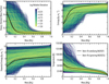 |
Fig. 1 Primordial heavy-element mass fraction (top left), specific entropy (top right), specific potential entropy (bottom left), and temperature (bottom right) as a function of mass for 4,250 randomly generated Jupiter models. The color scale indicates the quality of the fit to Jupiter’s present-day structure. The solid black lines represent our best-fit model that fulfills Eq. (1). The dotted black line represents the best-fit model without applying the BA2025 constraint. |
4 Discussion
The key uncertainties of this study are two-fold: Simplification in the numerical modeling and the reliability of Eq. (1). In the following, we first discuss the limitations of our computational framework and their implications for the interpretation of our Jupiter models. Finally, we evaluate the assumptions and reliability of the dynamical constraint derived from the Jovian moon system.
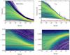 |
Fig. 2 Time evolution of the mean radius (top left), one-bar temperature (top right), J2 (bottom left), and J4 (bottom right) compared to present-day Jupiter (dashed red line). The line colors are the same as in Fig. 1. |
4.1 Planetary evolution
While planetary evolution models provide valuable insight into interior structure, they inevitably rely on approximations. In the following, we briefly discuss three key sources of uncertainty that may affect the quantitative details of our results.
First, we model convection using mixing-length theory (MLT; see Kippenhahn et al. 2012, and references therein). In this framework, energy and material are primarily transported by the largest rising and sinking fluid parcels, which travels a characteristic mixing length lmlt ∝ αH, where H is the pressure scale height and α is a free parameter typically on the order of unity. Material mixing is treated as a diffusive process, with a diffusion coefficient that also depends on α. Because convection is very efficient at removing both entropy and composition gradients, the details of MLT do not significantly affect the evolution within convective zones. However, whether a region becomes convective at all remains an open question, particularly in the context of oscillatory double-diffusive convection (ODDC), which can arise in layers that are Schwarzschild unstable but Ledoux stable (e.g., Kato 1966; Radko 2007; Rosenblum et al. 2011; Aurnou et al. 2020; Tulekeyev et al. 2024; Fuentes et al. 2024; Fuentes 2025). Our simulations do not model ODDC self-consistently. A more detailed treatment could therefore affect the structure and extent of Jupiter’s fuzzy core.
Second, our atmosphere model does not explicitly account for clouds or the detailed molecular composition of Jupiter’s atmosphere (e.g., Chen et al. 2023). While the observed conditions are approximated by adjusting the visible opacity in the semi-gray model of Guillot (2010), a fully self-consistent treatment would be preferable, as it reduces reliance on free parameters. In planetary evolution models, the atmosphere primarily regulates the planetary contraction and cooling rate. This cooling drives the gradual expansion of the convective envelope, which in turn governs the erosion of the primordial composition profile (Knierim & Helled 2024). A more realistic atmosphere model could constrain the cooling history more tightly, thereby narrowing the range of viable initial conditions. However, it would not affect the key conclusions of this study, which remain robust for reasonable atmospheric assumptions (see also Sect. 4.5 in Knierim & Helled 2024).
Third, the heavy elements are represented by an ideal mixture of water and rock. The assumption of ideal mixing itself introduces an uncertainty (Darafeyeu et al. 2024). In reality, Jupiter’s interior could include different compositions and a more complex distribution of heavy elements, with varying compositions and depth-dependent abundances. Finally, the equations of state for heavy elements are also uncertain under planetary conditions, which can affect the inferred interior structure (e.g., Howard et al. 2025).
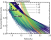 |
Fig. 3 Time evolution of normalized moment of inertia vs. radius for the sample of randomly generated Jupiter models. The line colors are the same as in Fig. 1. The colored regions indicate the primordial constraint of Eq. (1), where the labels indicate the resonance of Io with Amalthea (A) or Thebe (T), respectively. The black triangles mark Jupiter’s present-day radius and NMoI as estimated by Helled et al. (2011) and Ni (2018), respectively. The black square corresponds to the initial model from Sur et al. (2025b). |
4.2 Fine-tuning Jupiter
Within our sample, several models reproduce present-day Jupiter reasonably well, with relative differences below 1%. As discussed in Sect. 4.1, however, the detailed properties of an individual model remain sensitive to our specific assumptions. In practice, such models could be tuned to achieve a marginally better or worse fit, but this fine-tuning would not yield deeper physical insight, it would merely reflect the limitations of the numerical framework. Because the entire ensemble was computed under consistent assumptions, the robust outcome lies in the common trends that emerge across models rather than in any single realization. Our results should therefore be viewed as constraints on Jupiter’s interior in a general sense, not as a definitive, one-to-one prediction of its primordial structure.
4.3 The dynamical constraint
The main uncertainty in Eq. (1) lies in the assumption that Io’s primordial location coincided with the truncation radius of Jupiter’s CPD. While this radius represents a natural barrier to inward migration, it is not necessarily impenetrable. In particular, sufficiently massive outer companions can push inner bodies past the disk edge via resonant interactions – a mechanism proposed for the innermost planets of the TRAPPIST-1 system (Pichierri et al. 2024). Applied to the Galilean system, this scenario would imply that Io and Europa were pushed inside the CPD cavity by their more massive companion, Ganymede. Lacking an outer neighbor of comparable mass, Ganymede itself would have stalled near the disk’s truncation radius. In the most favorable case for this scenario – where Io is located at ξ = 4.11 – the three moons would be locked in their tightest possible configuration: a 4:2:1 mean-motion resonance. The truncation radius must then increase by a factor 42/3, yielding Rt = 10.35 RJ. Jupiter’s corresponding primordial spin, given by ![Mathematical equation: $\[\Omega_{\mathrm{J}}^{\dagger}=\chi \sqrt{G M_{\mathrm{J}} / R_{t}^{3}}\]$](/articles/aa/full_html/2026/02/aa56984-25/aa56984-25-eq20.png) (Batygin 2018), would be reduced by a factor of four compared to the baseline scenario. Angular momentum conservation requires that
(Batygin 2018), would be reduced by a factor of four compared to the baseline scenario. Angular momentum conservation requires that ![Mathematical equation: $\[I_{\mathrm{J}}^{\dagger} R_{\mathrm{J}}^{\dagger^{2}}\]$](/articles/aa/full_html/2026/02/aa56984-25/aa56984-25-eq21.png) increase by the same factor.
increase by the same factor.
However, as shown in Sect. 3, models with fuzzy cores naturally evolve toward Jupiter’s present-day structure, and thus represent at least an intermediate evolutionary state. An increase in the core entropy or a modification of the composition gradient would disrupt this agreement with current constraints. An increase in the envelope entropy does not alter the final structure – it merely delays cooling and prolongs the evolutionary pathway (see Knierim & Helled 2024). Therefore, the only viable way to reconcile our best-fit models with the required fourfold increase in ![Mathematical equation: $\[I_{\mathrm{J}}^{\dagger} R_{\mathrm{J}}^{\dagger^{2}}\]$](/articles/aa/full_html/2026/02/aa56984-25/aa56984-25-eq22.png) is by inflating the radiative envelope. Such an inflation reduces I, forcing R to increase at minimum by a factor of 2, but more likely far beyond that. Numerical experiments show that even at RJ† ≈ 3 RJ, the Kelvin-Helmholtz timescale of proto-Jupiter would be on the order of 5 × 10⁴ yr. Achieving inflation beyond that state would require an extreme internal energy and would evolve on unrealistically short timescales, rendering the solution physically implausible. Moreover, recent formation models of Amalthea and Thebe suggest that they were pushed in by Io (Brunton & Batygin 2025b,a). Hence, a proto-Jupiter larger than 4 RJ would have engulfed (and thus destroyed) these two moons. We therefore conclude that the CPD truncation radius could not have been this far out, and that it is unlikely that Io migrated into Jupiter’s magnetospheric cavity.
is by inflating the radiative envelope. Such an inflation reduces I, forcing R to increase at minimum by a factor of 2, but more likely far beyond that. Numerical experiments show that even at RJ† ≈ 3 RJ, the Kelvin-Helmholtz timescale of proto-Jupiter would be on the order of 5 × 10⁴ yr. Achieving inflation beyond that state would require an extreme internal energy and would evolve on unrealistically short timescales, rendering the solution physically implausible. Moreover, recent formation models of Amalthea and Thebe suggest that they were pushed in by Io (Brunton & Batygin 2025b,a). Hence, a proto-Jupiter larger than 4 RJ would have engulfed (and thus destroyed) these two moons. We therefore conclude that the CPD truncation radius could not have been this far out, and that it is unlikely that Io migrated into Jupiter’s magnetospheric cavity.
5 Conclusions
We identified the range of primordial interior structures that evolve toward present-day Jupiter while simultaneously satisfying dynamical constraints from Jupiter’s moon system – specifically, the inclinations of Amalthea and Thebe. Our key conclusions are:
The dynamical constraints from Amalthea and Thebe provide a valuable new handle on Jupiter’s primordial structure, helping to break degeneracies inherent in thermal evolution models alone;
Jupiter’s present-day structure is best reproduced by an initially warm (
![Mathematical equation: $\[s_{\text {core}}^{\dagger}\]$](/articles/aa/full_html/2026/02/aa56984-25/aa56984-25-eq23.png) ~ 5 kB mu−1), dilute core (
~ 5 kB mu−1), dilute core (![Mathematical equation: $\[Z_{\text {core}}^{\dagger}\]$](/articles/aa/full_html/2026/02/aa56984-25/aa56984-25-eq24.png) ~0.4), surrounded by a warm (
~0.4), surrounded by a warm (![Mathematical equation: $\[s_{\text {env}}^{\dagger}\]$](/articles/aa/full_html/2026/02/aa56984-25/aa56984-25-eq25.png) ~ 9.3 kB mu−1), moderately enriched envelope (
~ 9.3 kB mu−1), moderately enriched envelope (![Mathematical equation: $\[Z_{\text {env}}^{\dagger}\]$](/articles/aa/full_html/2026/02/aa56984-25/aa56984-25-eq26.png) ~0.05);
~0.05);The dilute core of present-day Jupiter is most likely a primordial feature – shaped during formation, not by subsequent evolution.
Overall, our results demonstrate the power of dynamical constraints to complement traditional structure modeling, and reinforce the view that Jupiter – and potentially gas giants more generally – is neither a homogeneous sphere of hydrogen and helium, nor a simple core plus envelope system. Rather, it is a complex, stratified object whose structure encodes the fingerprints of its formation. Fueled by upcoming space missions and unprecedented data, planetary science is poised to move from classification to explanation – to uncover not just what planets are, but also how they form and evolve.
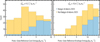 |
Fig. 4 Distributions of core entropy (left) and envelope entropy (right) before relaxing the composition gradient (i.e., at proto-solar composition) for models matching present-day Jupiter within 10%. Colors of the stacked histogram indicate whether or not the primordial constraint of BA2025 is fulfilled. Best-fit values for the constrained models are marked at the center of each panel. |
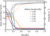 |
Fig. 5 Primordial heavy-element mass fraction (solid lines) and entropy (dotted lines) for the five best-fitting models that satisfy Eq. (1). |
Acknowledgements
We thank Ankan Sur, Roberto Tejada Arevalo, and Adam Burrows for kindly providing their Jupiter models. This work has been carried out within the framework of the National Centre of Competence in Research PlanetS supported by the Swiss National Science Foundation under grants 51NF40_182901, 51NF40_205606, and 215634. FCA is supported in part by Grant No. 2508843 from the National Science Foundation (USA) and by the Leinweber Institute for Theoretical Physics at the University of Michigan. KB is thankful for the support of the David and Lucile Packard Foundation, and the National Science Foundation (grant No. AST 2408867) as well as to Caltech and 3 CPE.
References
- Aurnou, J. M., Horn, S., & Julien, K. 2020, Phys. Rev. Res., 2, 043115 [NASA ADS] [CrossRef] [Google Scholar]
- Batygin, K. 2018, AJ, 155, 178 [NASA ADS] [CrossRef] [Google Scholar]
- Batygin, K., & Adams, F. C. 2025, Nat. Astron., 9, 835 [Google Scholar]
- Batygin, K., & Laughlin, G. 2015, Proc. Natl. Acad. Sci. U.S.A., 112, 4214 [NASA ADS] [CrossRef] [Google Scholar]
- Bolton, S. J., Lunine, J., Stevenson, D., et al. 2017, Space Sci. Rev., 213, 5 [Google Scholar]
- Brunton, I. R., & Batygin, K. 2025a, ApJ, 990, L11 [Google Scholar]
- Brunton, I. R., & Batygin, K. 2025b, ApJ, 991, 15 [Google Scholar]
- Chabrier, G., & Debras, F. 2021, ApJ, 917, 4 [NASA ADS] [CrossRef] [Google Scholar]
- Chen, Y.-X., Burrows, A., Sur, A., & Arevalo, R. T. 2023, ApJ, 957, 36 [NASA ADS] [CrossRef] [Google Scholar]
- Cozza, C., Nakano, K., Howard, S., et al. 2025, PRX, submitted [arXiv:2501.12925] [Google Scholar]
- Cumming, A., Helled, R., & Venturini, J. 2018, MNRAS, 477, 4817 [Google Scholar]
- Darafeyeu, V., Rimle, S., Mazzola, G., & Helled, R. 2024, ApJ, 975, 255 [Google Scholar]
- Fuentes, J. R. 2025, ApJ, 982, 44 [Google Scholar]
- Fuentes, J. R., Hindman, B. W., Fraser, A. E., & Anders, E. H. 2024, ApJ, 975, L1 [NASA ADS] [CrossRef] [Google Scholar]
- Guillot, T. 2005, AREPS, 33, 493 [NASA ADS] [Google Scholar]
- Guillot, T. 2010, A&A, 520, A27 [NASA ADS] [CrossRef] [EDP Sciences] [Google Scholar]
- Gupta, P., Atreya, S. K., Steffes, P. G., et al. 2022, PSJ, 3, 159 [Google Scholar]
- Hamilton, D. P., Proctor, A. L., & Rauch, K. P. 2001, in AAS/Division for Planetary Sciences Meeting Abstracts, 33, 25.04 [Google Scholar]
- Helled, R. 2023, A&A, 675, L8 [NASA ADS] [CrossRef] [EDP Sciences] [Google Scholar]
- Helled, R., & Stevenson, D. 2017, ApJ, 840, L4 [NASA ADS] [CrossRef] [Google Scholar]
- Helled, R., Anderson, J. D., Schubert, G., & Stevenson, D. J. 2011, Icarus, 216, 440 [Google Scholar]
- Helled, R., Stevenson, D. J., Lunine, J. I., et al. 2022, Icarus, 378, 114937 [NASA ADS] [CrossRef] [Google Scholar]
- Helled, R., Müller, S., & Knierim, H. 2025, A&A, 704, A253 [NASA ADS] [CrossRef] [EDP Sciences] [Google Scholar]
- Howard, S., Helled, R., & Müller, S. 2025, A&A, 693, L7 [NASA ADS] [CrossRef] [EDP Sciences] [Google Scholar]
- Jermyn, A. S., Bauer, E. B., Schwab, J., et al. 2023, ApJS, 265, 15 [NASA ADS] [CrossRef] [Google Scholar]
- Kato, S. 1966, PASJ, 18, 374 [NASA ADS] [Google Scholar]
- Kippenhahn, R., Weigert, A., & Weiss, A. 2012, Stellar Structure and Evolution (Springer-Verlag Berlin Heidelberg) [Google Scholar]
- Knierim, H., & Helled, R. 2024, ApJ, 977, 227 [Google Scholar]
- Knierim, H., & Helled, R. 2025, A&A, 698, L1 [NASA ADS] [CrossRef] [EDP Sciences] [Google Scholar]
- Kleine, T., Budde, G., Burkhardt, C., et al. 2020, Space Sci. Rev., 216, 55 [Google Scholar]
- Lozovsky, M., Helled, R., Rosenberg, E. D., & Bodenheimer, P. 2017, ApJ, 836, 227 [NASA ADS] [CrossRef] [Google Scholar]
- Meier, T., Reinhardt, C., Shibata, S., et al. 2025, ApJ, 988, 7 [Google Scholar]
- Morf, L. 2025, PyToF: a numerical implementation of the Theory of Figures algorithm (4th, 7th, 10th order) including barotropic differential rotation [Google Scholar]
- Morf, L., Müller, S., & Helled, R. 2024, A&A, 690, A105 [NASA ADS] [CrossRef] [EDP Sciences] [Google Scholar]
- Müller, S., Helled, R., & Cumming, A. 2020, A&A, 638, A121 [Google Scholar]
- Nettelmann, N., & Fortney, J. J. 2025, PSJ, 6, 98 [Google Scholar]
- Ni, D. 2018, A&A, 613, A32 [NASA ADS] [CrossRef] [EDP Sciences] [Google Scholar]
- Ni, D. 2019, A&A, 632, A76 [NASA ADS] [CrossRef] [EDP Sciences] [Google Scholar]
- Paxton, B., Bildsten, L., Dotter, A., et al. 2010, ApJS, 192, 3 [Google Scholar]
- Paxton, B., Cantiello, M., Arras, P., et al. 2013, ApJS, 208, 4 [Google Scholar]
- Paxton, B., Marchant, P., Schwab, J., et al. 2015, ApJS, 220, 15 [Google Scholar]
- Paxton, B., Schwab, J., Bauer, E. B., et al. 2018, ApJS, 234, 34 [NASA ADS] [CrossRef] [Google Scholar]
- Paxton, B., Smolec, R., Schwab, J., et al. 2019, ApJS, 243, 10 [Google Scholar]
- Pichierri, G., Morbidelli, A., Batygin, K., & Brasser, R. 2024, Nat. Astron., 8, 1408 [NASA ADS] [CrossRef] [Google Scholar]
- Pollack, J. B., Hubickyj, O., Bodenheimer, P., et al. 1996, Icarus, 124, 62 [NASA ADS] [CrossRef] [Google Scholar]
- Radko, T. 2007, J. Fluid Mech., 577, 251 [Google Scholar]
- Rosenblum, E., Garaud, P., Traxler, A., & Stellmach, S. 2011, ApJ, 731, 66 [NASA ADS] [CrossRef] [Google Scholar]
- Schöttler, M., & Redmer, R. 2018, Phys. Rev. Lett., 120, 115703 [CrossRef] [Google Scholar]
- Shibata, S., Helled, R., & Kobayashi, H. 2023, MNRAS, 519, 1713 [Google Scholar]
- Stevenson, D. J. 1982, AREPS, 10, 257 [Google Scholar]
- Stevenson, D. J. 1985, Icarus, 62, 4 [NASA ADS] [CrossRef] [Google Scholar]
- Stevenson, D. J., & Salpeter, E. E. 1977, ApJS, 35, 239 [NASA ADS] [CrossRef] [Google Scholar]
- Stevenson, D. J., Bodenheimer, P., Lissauer, J. J., & D’Angelo, G. 2022, PSJ, 3, 74 [NASA ADS] [Google Scholar]
- Sur, A., Su, Y., Tejada Arevalo, R., Chen, Y.-X., & Burrows, A. 2024, ApJ, 971, 104 [Google Scholar]
- Sur, A., Burrows, A., & Tejada Arevalo, R. 2025a, ApJ, 994, 186 [Google Scholar]
- Sur, A., Tejada Arevalo, R., Su, Y., & Burrows, A. 2025b, ApJ, 980, L5 [Google Scholar]
- Tejada Arevalo, R., Sur, A., Su, Y., & Burrows, A. 2025, ApJ, 979, 243 [Google Scholar]
- Tulekeyev, A., Garaud, P., Idini, B., & Fortney, J. J. 2024, PSJ, 5, 190 [Google Scholar]
- Vazan, A., Kovetz, A., Podolak, M., & Helled, R. 2013, MNRAS, 434, 3283 [NASA ADS] [CrossRef] [Google Scholar]
- Vazan, A., Helled, R., & Guillot, T. 2018, A&A, 610, L14 [NASA ADS] [CrossRef] [EDP Sciences] [Google Scholar]
- Wahl, S. M., Hubbard, W. B., Militzer, B., et al. 2017, Geophys. Res. Lett., 44, 4649 [CrossRef] [Google Scholar]
- Zapolsky, H. S., & Salpeter, E. E. 1969, ApJ, 158, 809 [Google Scholar]
- Zharkov, V. N., & Trubitsyn, V. P. 1978, Physics of Planetary Interiors (Tucson, Ariz.: Pachart Pub. House) [Google Scholar]
Appendix A Rotation in MESA
In MESA, rotation is implemented using the shellular approximation (Paxton et al. 2013). Rather than solving the full threedimensional structure, the object is divided into isobars, and the one-dimensional structure equations are solved as volume-averaged quantities over these isobars. Rotation enters explicitly into both the momentum balance and energy transport equations.
Angular momentum transport is treated as a diffusion process. While MESA offers several prescriptions for differential rotation, for simplicity we assume solid-body rotation throughout this study.
Similarly, although MESA includes models for rotationally induced mixing, magnetic field generation, or mass loss, these are primarily calibrated for stars and involve free parameters that are unknown for planets. We therefore omit these additional effects. Instead, we use the polar and equatorial radii, together with the rotation rate, to compute the gravitational moments and moment of inertia of the model.
Rotation is initialized using relax_initial_omega, which sets a uniform rotation rate throughout the planet at the start of our calculations.
Appendix B Random model generation
We construct the initial heavy-element distribution Z(m) using a generalized logistic profile,
![Mathematical equation: $\[Z(m)=Z_{\text {core }}^{\dagger}-\frac{Z_{\text {core }}^{\dagger}-Z_{\text {env }}^{\dagger}}{1+\exp \left[\alpha_Z\left(m-m_{\text {mid }}\right)\right]},\]$](/articles/aa/full_html/2026/02/aa56984-25/aa56984-25-eq27.png) (B.1)
(B.1)
where ![Mathematical equation: $\[Z_{\text {core}}^{\dagger}\]$](/articles/aa/full_html/2026/02/aa56984-25/aa56984-25-eq28.png) and
and ![Mathematical equation: $\[Z_{\text {env}}^{\dagger}\]$](/articles/aa/full_html/2026/02/aa56984-25/aa56984-25-eq29.png) denote the heavy-element mass fractions in the limits m → −∞ and m → ∞, respectively. The composition steepness parameter αZ controls how steeply the heavy-element mass fraction transitions between these two regimes, and mmid specifies its midpoint in mass coordinate. For sufficiently large αZ,
denote the heavy-element mass fractions in the limits m → −∞ and m → ∞, respectively. The composition steepness parameter αZ controls how steeply the heavy-element mass fraction transitions between these two regimes, and mmid specifies its midpoint in mass coordinate. For sufficiently large αZ, ![Mathematical equation: $\[Z_{\text {core}}^{\dagger}\]$](/articles/aa/full_html/2026/02/aa56984-25/aa56984-25-eq30.png) and
and ![Mathematical equation: $\[Z_{\text {env}}^{\dagger}\]$](/articles/aa/full_html/2026/02/aa56984-25/aa56984-25-eq31.png) may be interpreted as the heavy-element fractions at the center and in the outer envelope.
may be interpreted as the heavy-element fractions at the center and in the outer envelope.
The specific entropy profile at proto-solar composition, i.e., before relaxing the composition profile, is parameterized as
![Mathematical equation: $\[s^{\odot}(m)=s_{\mathrm{core}}^{\odot}+\left(\frac{m}{M}\right)^{\alpha_s}\left(s_{\mathrm{env}}^{\odot}-s_{\mathrm{core}}^{\odot}\right),\]$](/articles/aa/full_html/2026/02/aa56984-25/aa56984-25-eq32.png) (B.2)
(B.2)
where the entropy steepness parameter αs determines the slope between the core entropy ![Mathematical equation: $\[s_{\text {core}}^{\odot}\]$](/articles/aa/full_html/2026/02/aa56984-25/aa56984-25-eq33.png) and the envelope entropy
and the envelope entropy ![Mathematical equation: $\[s_{\text {env}}^{\odot}\]$](/articles/aa/full_html/2026/02/aa56984-25/aa56984-25-eq34.png) . This form allows for a wide range of initial stratifications, from nearly isentropic interiors to steep entropy gradients, similar to those found in Cumming et al. (2018).
. This form allows for a wide range of initial stratifications, from nearly isentropic interiors to steep entropy gradients, similar to those found in Cumming et al. (2018).
To explore a broad space of initial conditions, we draw parameters from wide ranges: ![Mathematical equation: $\[Z_{\text {core}}^{\dagger}\]$](/articles/aa/full_html/2026/02/aa56984-25/aa56984-25-eq35.png) uniformly between 0.1 and 1,
uniformly between 0.1 and 1, ![Mathematical equation: $\[Z_{\text {env}}^{\dagger}\]$](/articles/aa/full_html/2026/02/aa56984-25/aa56984-25-eq36.png) uniformly between Z⊙ and 0.1, mmid uniformly between 0 and 0.5 MJ, αZ log-uniformly between 1 and 200,
uniformly between Z⊙ and 0.1, mmid uniformly between 0 and 0.5 MJ, αZ log-uniformly between 1 and 200, ![Mathematical equation: $\[s_{\text {core}}^{\odot}\]$](/articles/aa/full_html/2026/02/aa56984-25/aa56984-25-eq37.png) uniformly between 7.0 and 10 kB mu−1,
uniformly between 7.0 and 10 kB mu−1, ![Mathematical equation: $\[s_{\text {env}}^{\odot}\]$](/articles/aa/full_html/2026/02/aa56984-25/aa56984-25-eq38.png) uniformly between
uniformly between ![Mathematical equation: $\[s_{\text {core}}^{\odot}\]$](/articles/aa/full_html/2026/02/aa56984-25/aa56984-25-eq39.png) and 11 kB mu−1, and αs uniformly between 0.3 and 2.0. The total angular momentum is also varied by a factor of two around a reference value corresponding to a NMoI of 0.265 (Helled et al. 2011). Inside MESA, we first relax the new angular momentum, then the entropy profile, and finally the composition profile before evolving the system.
and 11 kB mu−1, and αs uniformly between 0.3 and 2.0. The total angular momentum is also varied by a factor of two around a reference value corresponding to a NMoI of 0.265 (Helled et al. 2011). Inside MESA, we first relax the new angular momentum, then the entropy profile, and finally the composition profile before evolving the system.
Appendix C Constraints on the primordial composition gradient
Figure C.1 shows that, in contrast to the entropy results in Fig. 4, other primordial parameters are only weakly affected by the BA2025 constraint. Models satisfying the BA2025 constraint tend to favor less massive cores, while showing no strong preference for the steepness of the composition profile. The distributions of core and envelope heavy-element fractions remain similar to those of the unconstrained case.
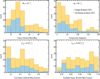 |
Fig. C.1 Same as Fig. 4 but for the total heavy-element mass (top left), αZ (top right), |
![Mathematical equation: $\[Z_{\text {core}}^{\dagger}\]$](/articles/aa/full_html/2026/02/aa56984-25/aa56984-25-eq40.png)
![Mathematical equation: $\[Z_{\text {env}}^{\dagger}\]$](/articles/aa/full_html/2026/02/aa56984-25/aa56984-25-eq41.png)
All Figures
|
Fig. 1 Primordial heavy-element mass fraction (top left), specific entropy (top right), specific potential entropy (bottom left), and temperature (bottom right) as a function of mass for 4,250 randomly generated Jupiter models. The color scale indicates the quality of the fit to Jupiter’s present-day structure. The solid black lines represent our best-fit model that fulfills Eq. (1). The dotted black line represents the best-fit model without applying the BA2025 constraint. |
| In the text | |
|
Fig. 2 Time evolution of the mean radius (top left), one-bar temperature (top right), J2 (bottom left), and J4 (bottom right) compared to present-day Jupiter (dashed red line). The line colors are the same as in Fig. 1. |
| In the text | |
|
Fig. 3 Time evolution of normalized moment of inertia vs. radius for the sample of randomly generated Jupiter models. The line colors are the same as in Fig. 1. The colored regions indicate the primordial constraint of Eq. (1), where the labels indicate the resonance of Io with Amalthea (A) or Thebe (T), respectively. The black triangles mark Jupiter’s present-day radius and NMoI as estimated by Helled et al. (2011) and Ni (2018), respectively. The black square corresponds to the initial model from Sur et al. (2025b). |
| In the text | |
|
Fig. 4 Distributions of core entropy (left) and envelope entropy (right) before relaxing the composition gradient (i.e., at proto-solar composition) for models matching present-day Jupiter within 10%. Colors of the stacked histogram indicate whether or not the primordial constraint of BA2025 is fulfilled. Best-fit values for the constrained models are marked at the center of each panel. |
| In the text | |
|
Fig. 5 Primordial heavy-element mass fraction (solid lines) and entropy (dotted lines) for the five best-fitting models that satisfy Eq. (1). |
| In the text | |
|
Fig. C.1 Same as Fig. 4 but for the total heavy-element mass (top left), αZ (top right), |
| In the text | |
Current usage metrics show cumulative count of Article Views (full-text article views including HTML views, PDF and ePub downloads, according to the available data) and Abstracts Views on Vision4Press platform.
Data correspond to usage on the plateform after 2015. The current usage metrics is available 48-96 hours after online publication and is updated daily on week days.
Initial download of the metrics may take a while.