| Issue |
A&A
Volume 706, February 2026
|
|
|---|---|---|
| Article Number | A152 | |
| Number of page(s) | 13 | |
| Section | Stellar atmospheres | |
| DOI | https://doi.org/10.1051/0004-6361/202557071 | |
| Published online | 11 February 2026 | |
Spectral evolution of hot hybrid white dwarfs
II. Photometry
1
Landessternwarte Heidelberg, Zentrum für Astronomie, Ruprecht-Karls-Universität,
Königstuhl 12,
69117
Heidelberg,
Germany
2
Institut für Astronomie und Astrophysik, Kepler Center for Astro and Particle Physics, Eberhard Karls Universität,
Sand 1,
72076
Tübingen,
Germany
3
Instituto de Astrofìsica de Canarias,
38205
La Laguna, Tenerife,
Spain
4
Departamento de Astrofìsica, Universidad de La Laguna,
38206
La Laguna, Tenerife,
Spain
5
Institut für Physik und Astronomie, Universität Potsdam,
Haus 28, Karl-Liebknecht-Str. 24/25,
14476
Potsdam,
Germany
★ Corresponding author: This email address is being protected from spambots. You need JavaScript enabled to view it.
Received:
2
September
2025
Accepted:
29
October
2025
Abstract
We present a photometric analysis of 19 DA and 13 DAO white dwarfs (WDs) with effective temperatures exceeding 60 000 K, building on the spectral analysis reported in the first paper of this two-part study. By examining archival light curves for periodic signals, we identify that four of the 32 objects (13−4+8%) exhibit photometric variability. Spectral energy distribution (SED) fitting allowed us to derive radii, luminosities, and gravity masses, as well as to characterise the infrared excesses observed in six sources. A notable discovery is the identification of a 1.87 d period in the ZTF light curves of WD 1342+443 and weak emission lines in the optical spectra of this star, which strongly indicate an irradiation effect system. Our SED fit indicates the presence of cool dust, which must be located farther from the star, and that any companion with a spectral type earlier than L2.0 would appear in the SED. This leads us to speculate that WD 1342+443 might have an irradiated, sub-stellar companion. We also highlight that we uncovered, for the first time, a 4.23 d photometric period in the well-known, close DA+dM binary WD 0232+035, based on TESS data. We find that the phase and amplitude of the light curve variations are consistent with expectations from an irradiation effect. Intriguingly, we detected an additional, mysterious period at 1.39 days, which is approximately one-third of the orbital period. Moreover, we revisited the longstanding discrepancy between Kiel and gravity masses for the hottest WDs. To address this, we explored fully metal line blanketed model atmospheres as a potential solution, contrasting them with the results from pure-hydrogen and hydrogen-helium models. Our results show that including metal opacities does not resolve the discrepancy – in fact, it slightly deteriorates the agreement. Finally, we reaffirm the previously observed correlation between helium abundance and luminosity.
Key words: binaries: general / stars: variables: general / white dwarfs
© The Authors 2026
 Open Access article, published by EDP Sciences, under the terms of the Creative Commons Attribution License (https://creativecommons.org/licenses/by/4.0), which permits unrestricted use, distribution, and reproduction in any medium, provided the original work is properly cited.
This article is published in open access under the Subscribe to Open model. This email address is being protected from spambots. You need JavaScript enabled to view it. to support open access publication.
1 Introduction
Large photometric surveys and missions are generally devised for specific research interests in astronomy, such as exploring transient phenomena (Law et al. 2009), monitoring asteroids and comets (Tonry et al. 2018), discovering exoplanets (Ricker et al. 2015), or investigating stellar populations in our Galaxy (Alonso-García et al. 2018). However, the obtained data are useful for purposes other than their intended science objectives, from which white dwarf (WD) studies also benefit substantially. For instance, photometry of a large sample of WDs can be used as a benchmark to validate theories of their internal physical processes (Bédard et al. 2024).
On the one hand, time-series observations uncover important aspects of stars, e.g., stellar activity and multiplicity, pulsations, magnetic fields, and rotation. Excluding GW Vir pulsators with inherently hydrogen-deficient atmospheres (Werner & Herwig 2006), close binarity is perhaps the first suspected mechanism that leads to photometric variability in hot WDs (Steen et al. 2024; Oliveira da Rosa et al. 2024). In particular, so-called irradiation effect systems, in which the phase-varying projection of the cooler companion leads to periodic variations in brightness, are well documented (Brinkworth et al. 2006; Aungwerojwit et al. 2007; Parsons et al. 2010). In these systems, the rotational period of the cool companion is expected to be synchronised to the orbital period (Nebot Gómez-Morán et al. 2011). In recent years, the first indications of bright spots on hot WDs have been reported (Reindl et al. 2019, 2021, 2023). The partly unusual light curve shapes of these objects are thought to be caused by bright spots on the surfaces of these stars, which in turn are believed to form through interactions of metals with weak magnetic fields (Hermes et al. 2017b). Furthermore, it is speculated that the onset of diffusion could be an additional decisive factor in the development of spots on hot WDs (Reindl et al. 2023).
On the other hand, photometry acquired in multiple bands enables us to construct spectral energy distributions (SEDs). By fitting synthetic spectra to the observed photometry, we can derive the angular diameter of the source. This, in combination with high-precision parallaxes provided by the Gaia space mission (Gaia Collaboration 2016, 2018, 2023), yields stellar radii and, in combination with previously derived surface gravities (log g), also masses independently of theoretical evolutionary calculations. This method is widely used to derive fundamental parameters for large samples of both H-rich and H-deficient WDs (Bergeron et al. 2019; Genest-Beaulieu & Bergeron 2019; Tremblay et al. 2019). It has been used to construct a (semi)empirical initial–final mass relation (Barnett et al. 2021; Cunningham et al. 2024) and to test theoretical predictions of the mass–radius relationship (Bédard et al. 2017; Tremblay et al. 2017; Raddi et al. 2025). By fitting the SED, it is also possible to determine the effective temperature (Teff), which remains a free parameter in the fitting procedure along with the angular diameter (Gentile Fusillo et al. 2019, 2021). However, a larger discrepancy in the atmospheric parameters of hot WDs can be identified between photometry and spectroscopy (Bergeron et al. 2019; Tremblay et al. 2019). Hot WD masses derived from a combination of photometry and spectroscopy also show disagreement with those inferred from evolutionary tracks (Löbling et al. 2020; Reindl et al. 2023).
Besides offering a method to derive stellar radii and masses independently of evolutionary models, SED fitting also allows us to search for an infrared (IR) excess. Such an excess can indicate the presence of a cooler (sub-)stellar companion, or hot and cold dust discs (Chu et al. 2011; De Marco et al. 2013; Reindl et al. 2024).
In this paper, we finalise the study reported in Filiz et al. (2024, hereafter Paper I), which focuses on the spectral evolution of hot DA and DAO (hybrid) WDs via ultraviolet (UV) and optical spectroscopy. Here, we present a photometric analysis of our sample of WDs that was introduced in Paper I. In Sect. 2, we introduce the time-series observations and the analysis method. In Sect. 3, we explain our SED fitting process. We discuss the implications of our results in Sect. 4 and conclude with a brief summary in Sect. 5.
2 Light curves
2.1 Datasets
We collected archival light curves from several surveys, as listed below. All 32 targets from Paper I have at least one archival light curve.
TESS. The Transiting Exoplanet Survey Satellite (TESS) missions comprised individual sectors that were scanned for two orbits (≈27.4 d). The satellite is equipped with a red-optical bandpass covering the range 6000–10 000 Å. The Science Processing Operations Center (SPOC) pipeline (Jenkins et al. 2016) provides pre-processed light curves, which we acquired from the Mikulski Archive for Space Telescopes (MAST)1 along with their corresponding target pixel files (TPFs). We used 2 min and 20 s cadence light curves and the pre-search data conditioning simple aperture photometry (PDCSAP) fluxes from which long-term trends have been removed. Two-minute cadence observations are available for all objects, whereas only 21 of them have 20 s cadence data.
ZTF. The Zwicky Transient Facility (ZTF; Bellm et al. 2019; Masci et al. 2019) survey is conducted with the Palomar 48-inch telescope at the Palomar Observatory, which scans the northern sky with a wide field of view (FOV; 47 deg2) at 2 d cadence. We retrieved time-series data with an exposure time of 30 s in the g and r-band for 21 objects, while i-band observations are available for only ten objects. The data were obtained from the 22nd data release (DR22), spanning March 2018 to June 2024. CSS. The Catalina Sky Survey (CSS; Drake et al. 2009) is designed to detect and track near-Earth objects, which employs three 1-m class telescopes located at the Steward Observatory of the University of Arizona. Spanning from 11.5 to 21.5 magnitudes, the second data release of the CSS contains V-band photometry of objects in the range of −75° < δ < 70° and |b| > 15°. Observations are separated into fields, with each field observed four times every 30 minutes. We found CSS light curves for 25 objects, but most observations do not have enough data points to detect variability.
ATLAS. The Asteroid Terrestrial-impact Last Alert System (ATLAS, Tonry et al. 2018) is operated with four automated 0.5 m telescopes (located in Hawaii, South Africa, and Chile) that contain ‘cyan’ (4200–6500 Å) and ‘orange’ (5600–8200 Å) bandpass filters. We found ATLAS light curves only for two of our objects.
Gaia multi-epoch photometry. The third data release of the Gaia mission (Gaia Collaboration 2023) contains multi-epoch broadband photometry in G, GBP, and GRP bands, in which variable objects were detected using statistical and machine-learning methods (Eyer et al. 2023). Only one object2 in our sample has Gaia multi-epoch photometry.
2.2 Analysis
Our light curve analysis method builds upon the procedure described in Reindl et al. (2021, 2023, 2024). We used VAR-TOOLS software (Hartman & Bakos 2016) and calculated a generalised Lomb-Scargle (LS) periodogram (Zechmeister & Kürster 2009; Press et al. 1992) to detect periodic sinusoidal signals. We relied on the false alarm probability (FAP) of the periodic signal to classify variability. If the periodic signal from a particular object showed log(FAP) ≤ −4, we classified that object as variable. In cases where the periodogram generated more than one significant period for an object, we removed the strongest periodic signal (including its harmonics and sub-harmonics) from the light curve and recalculated the periodogram. This procedure was repeated until no periodic signal could be found above the set variability threshold (log(FAP) ≤ −4). We measured peak-to-peak amplitudes by fitting a harmonic series to each light curve, defined as the difference between the maximum and minimum of the fit.
The first run of the LS periodogram on the 2 min cadence TESS data revealed periodic variability for 16 objects. Eight of these objects still showed variability even after the third whitening cycle. In addition, only seven of the variable candidates have a value of crowdsap ≥ 0.9, with the median value being 0.74; this parameter in the TPF header estimates the fraction of the collected light in the aperture that comes from the target. In fact, TESS has a large plate scale (21″/pixel), which makes crowding problems unavoidable. Therefore, validating the source of the periodic signal obtained from the light curve is essential.
We inspected the TPFs of the 16 candidate variables mentioned above in all sectors using tpfplotter3 (Aller et al. 2020) to detect possible blending sources or nearby contaminants in the aperture. The TPF plots show the aperture mask used by the pipeline and all sources in the TPF file with a magnitude difference down to Δm = 6. For only nine objects were no blending sources detected in the aperture of all sectors, whereas in two cases at least one sector did not reveal any contamination in the aperture. However, the absence or scarcity of contamination does not directly imply that the target object is the source of the periodic signal (Aller et al. 2024). Therefore, we used TESS_localize4 (Higgins & Bell 2023), which locates the source of variability on the sky for a given set of frequencies and TESS pixels, as well as the most likely Gaia sources within the selected TPF. For detection to be statistically significant, the height parameter should be less than 20% (equivalent of 5 σ, Higgins & Bell 2023). Consequently, only two objects (WD 0232+035 and WD 2350–706) were attributed to the detected signal. The same procedure was applied to the 20 s cadence data, but the periodogram reproduced the same periods as the 2 min light curves for only WD 0232+035 and WD 0311+480. However, in all sectors for both datasets, TESS_localize was unable to identify WD 0311+480 as the source of variability or statistically associate the detected signal with any other Gaia source.
We identified periodic signals for only two objects (WD 1056+516 and WD 1342+443) in the ZTF light curves. Both stars show the same periods in the g- and r-bands, but no variability is found in the i-band (229 and 463 data points, respectively). WD 1056+516 does not show variability in the TESS data. In contrast, we find variability in the TESS data for WD 1342+443. However, the period detected in the TESS data does not match that found in the ZTF data and TESS_localize confirms that WD 1342+443 is not the source of the signal detected in the TESS data. Given that both objects are fainter than G = 16.6 mag and that TESS is designed for objects brighter than 15 mag, this result is not surprising. Fig. 1 shows phase folded light curves of the photometrically variable objects. An overview of the periods and amplitudes derived from the available datasets is shown in Table 1.
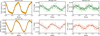 |
Fig. 1 Phase-averaged TESS (orange) and phase-averaged ZTF (green and red) light curves of the variable objects. Peak-to-peak amplitudes were measured by fitting a harmonic series, shown by the black lines. |
3 SED fits
We used the χ2 fitting routine explained in Heber et al. (2018) and Irrgang et al. (2021) to determine the radius, R, luminosity, L, and gravity mass, Mgrav, of each sample object. In essence, the procedure converts the model spectra to filter-averaged magnitudes and compares them with the photometric data collected from several surveys and catalogues, including Gaia (Riello et al. 2021), the Galaxy Evolution Explorer (GALEX; Martin et al. 2005; Bianchi et al. 2017), the Panoramic Survey Telescope and Rapid Response System (Pan-STARRS; Flewelling et al. 2020), Two Micron All Sky Survey (2MASS; Skrutskie et al. 2006), Sloan Digital Sky Survey (SDSS; Alam et al. 2015), the Spitzer Space Telescope (Fazio et al. 2004; Rieke et al. 2004), the Wide-field Infrared Survey Explorer (WISE; Wright et al. 2010; Schlafly et al. 2019; Marocco et al. 2021), Skymapper (Onken et al. 2019), the UK Infra-Red Telescope (UKIRT) Hemisphere Survey (UHS; Dye et al. 2018) and the Visible and Infrared Survey Telescope Survey (VISTA; McMahon et al. 2013). While we fixed the atmospheric parameters (effective temperature, Teff, surface gravity, log g, and He abundance) to the values determined in Paper I, the angular diameter, Θ, and the colour excess, E(44–55), remained free parameters. We adopted the interstellar reddening law of Fitzpatrick et al. (2019) with an extinction coefficient of R55 = 3.02, which uses E(44–55) measured with monochromatic filters at 4400 and 5500 Å, rather than the Johnson B and V filters used in E(B–V). For high Teff, such as our sample objects, E(44–55) is indistinguishable from E(B–V).
We relied on Gaia parallaxes to calculate the stellar parameters, which were corrected for their zero-point offset according to Lindegren et al. (2021). Parallax uncertainties were corrected with the function suggested by El-Badry et al. (2021). The radii were then calculated as R = Θ/ 2ϖ, using Θ derived from the SED fitting and Gaia parallaxes (ϖ). Using the spectroscopic values (Teff and log g) from Paper I, we derived the luminosities as L/L⊙ = (R/R⊙)2 (Teff/Teff,⊙)4 and gravity masses as Mgrav = gR2/G, where G is the gravitational constant.
We followed two different procedures to calculate R and Mgrav using SED fitting. First, we used the model flux of each object from Paper I, computed with the Tübingen Model-Atmosphere package (TMAP5; Werner & Dreizler 1999; Werner et al. 2003, 2012), since creating an extensive grid of fully metal line blanketed models is computationally expensive (see Paper I). Then, to test the effects of metals on the SED fits, we used the pure H and H+He model grids of Reindl et al. (2023) for the DA and DAO WDs, respectively. Table A.1 lists the radii, luminosities, gravity masses, and colour excesses derived using the former method. The differences between these results and those obtained using the metal-free models are discussed in further detail in Sect. 4.
We find that two DAO and four DA WDs in our sample exhibit an IR excess. For WD 1342+443 and WD 2218+706, we performed a multi-component fit using the model fluxes obtained in Paper I, together with one or two blackbody components. The other four objects that exhibit an IR excess are already known binaries. For these objects, instead of the blackbody components, we included PHOENIX models (Husser et al. 2013) spanning from 500 to 55 000 Å and temperatures 2300 K ≤ Teff ≤ 15 000 K. Figure 2 depicts the SED fits for sample objects with IR excess. For comparison, the top row shows one DAO and one DA WD without IR excess. The Teff and R of the IR sources are listed in Table 1.
Names, spectral types, observed bands, false alarm probabilities, periods, and peak–to–peak amplitudes of the variable objects, as well as the temperatures, radii, and surface ratios of the IR-excess sources.
4 Discussion
4.1 Variability and IR excess
For all 32 WDs in our sample, at least one archival light curve was available, and four objects were found to be photometrically variable. This implies a variability rate of ![Mathematical equation: $\[13_{-4}^{+8}\]$](/articles/aa/full_html/2026/02/aa57071-25/aa57071-25-eq16.png) %, which agrees with the variability rate of normal hot, H-rich WDs that do not exhibit the ultra-high excitation (UHE) phenomenon, of
%, which agrees with the variability rate of normal hot, H-rich WDs that do not exhibit the ultra-high excitation (UHE) phenomenon, of ![Mathematical equation: $\[14_{-3}^{+6}\]$](/articles/aa/full_html/2026/02/aa57071-25/aa57071-25-eq17.png) % as reported by Reindl et al. (2021). In the following paragraphs, we discuss stars that are either (possibly) photometrically variable or show IR excess, considering the origin of the variability and/or the excess.
% as reported by Reindl et al. (2021). In the following paragraphs, we discuss stars that are either (possibly) photometrically variable or show IR excess, considering the origin of the variability and/or the excess.
WD 0232+035. Also known as Feige 24, WD 0232+035 is one of the most studied hot DA WDs, with its close binary nature long established (Greenstein & Eggen 1966). Contamination by the irradiated M dwarf is evident in the optical spectra as photospheric absorption (mainly TiO absorption bands) and chromospheric Balmer emission. In previous studies, phase-resolved spectroscopy in the optical and UV enabled the determination of the radial velocity (RV) curves of the M-dwarf and the WD, respectively, yielding an orbital period of 4.23 d (Vennes et al. 1991; Vennes & Thorstensen 1994; Gianninas et al. 2011; Guo et al. 2015).
We used PHOENIX models to reproduce the IR excess in the SED (Fig. 2), resulting in Teff = ![Mathematical equation: $\[3710_{-60}^{+70}\]$](/articles/aa/full_html/2026/02/aa57071-25/aa57071-25-eq18.png) K and R = 0.395 ± 0.011 R⊙ for the companion. This radius is slightly lower than the average radius of an M dwarf with the corresponding Teff (Cifuentes et al. 2020). Kawka et al. (2008) reported R = 0.43 ± 0.02 R⊙ for the secondary and classified it as an M2 dwarf.
K and R = 0.395 ± 0.011 R⊙ for the companion. This radius is slightly lower than the average radius of an M dwarf with the corresponding Teff (Cifuentes et al. 2020). Kawka et al. (2008) reported R = 0.43 ± 0.02 R⊙ for the secondary and classified it as an M2 dwarf.
We find that the TESS light curve of this object exhibits a 4.23 d variability, which can be detected in both 2 min and 20 s cadence data. The same period is also present in the o-band ATLAS light curve, but not in the c-band, possibly due to a low number of data points. Therefore, we phased the c-band light curve to the period detected in the o-band. Heinze et al. (2018) reported a period of 8.45 d from the ATLAS data and listed the variability as dubious. The LS periodogram on CSS data yielded 0.81 d as the strongest signal (log(FAP) = −10.75). However, 4.37 d is also one of the five most significant detected signals (log(FAP) = −9.28), to which we phased the CSS light curve. Moreover, the amplitude measured in the CSS light curves is not consistent with those determined from the TESS and ATLAS data.
Although light variation was previously detected with the Hubble Space Telescope (HST) Fine Guidance Sensor 3 (Benedict et al. 2000), to the best of our knowledge, the 4.23 d photometric period is reported here for the first time and is consistent with the system’s orbital period inferred from phase-resolved spectroscopy (Thorstensen et al. 1978; Vennes et al. 1991; Vennes & Thorstensen 1994).
The Hα emission varies with orbital phase, as expected for an irradiation(reflection) effect system; however, the shape of the light curve of WD 0232+035 (Fig. 1, lower left panel) does not resemble this at first glance (Schaffenroth et al. 2018, see their Fig. 1). In contrast, the observed saw-tooth light curve morphology is often indicative of rotational modulation due to spots (Reindl et al. 2021). Interestingly, the light curve morphology does not remain constant throughout the TESS observations (Fig. 3), albeit with seemingly periodic repetitions (e.g. data from the start of sector 4, Fig. 3 upper panel, present a similar light curve morphology as the data from sector 71, Fig. 3 lower panel). Fitting and subtracting the dominant 4.23 d periodicity to the light curve using Period04 (Lenz & Breger 2005) reveals a second statistically significant periodicity at 1.39 d (approximately one third of the orbital period). The beating of these two signals likely causes the variation in light curve morphology.
A simulated light curve created with Phoebe2 (Prša et al. 2016; Conroy et al. 2020) suggests that the amplitude and phasing of the photometric variability at the orbital period may be consistent with irradiation. However, the origin of the shorter, lower amplitude 1.39 d periodicity is less clear. It may be due to spots, but this would imply that the spotted component of the binary is not tidally locked but rather rotating super-synchronously, which is not generally encountered in post-common envelope binaries (Nebot Gómez-Morán et al. 2011). We note that by respectively convolving the flux contributions of the WD and M-dwarf with the TESS spectral response function, we find that both components contribute equally to the observed flux in the TESS band. Intriguingly, the WD-main sequence (MS) binary LAMOST J172900.17+652952.8 was found to display somewhat similar variability, attributed by Zheng et al. (2022, see their Fig. 5) to strong stellar activity of the MS companion.
WD 0851+090. We did not detect any photometric variability for the DAO-type central star of planetary nebula (CSPN) Abell 31, consistent with the findings of Aller et al. (2024) based on their analysis of TESS light curves. However, we find an IR excess for this object (Fig. 2), whose origin had previously been attributed to an M4V companion (Ciardullo et al. 1999; Frew 2008; De Marco et al. 2013). We therefore performed a multi-component fit using the PHOENIX grid. We derive Teff = ![Mathematical equation: $\[2920_{-380}^{+210}\]$](/articles/aa/full_html/2026/02/aa57071-25/aa57071-25-eq19.png) K and R =
K and R = ![Mathematical equation: $\[0.26_{-0.04}^{+0.04}\]$](/articles/aa/full_html/2026/02/aa57071-25/aa57071-25-eq20.png) R⊙ for the cool companion, values that are comparable to the average parameters of an M5 dwarf (Cifuentes et al. 2020). The system is not resolved by Gaia, but Ciardullo et al. (1999) derived a separation of 0.26 arcsec using HST imaging. Using the updated Gaia eDR3 parallax (ϖGaia = 1.86 mas), we calculate a separation of 140 AU, which implies that the system is wide but physically bound and most likely did not undergo an interaction phase.
R⊙ for the cool companion, values that are comparable to the average parameters of an M5 dwarf (Cifuentes et al. 2020). The system is not resolved by Gaia, but Ciardullo et al. (1999) derived a separation of 0.26 arcsec using HST imaging. Using the updated Gaia eDR3 parallax (ϖGaia = 1.86 mas), we calculate a separation of 140 AU, which implies that the system is wide but physically bound and most likely did not undergo an interaction phase.
WD 1056+516. This DA WD is one of the two objects that show photometric variability in the ZTF dataset. Both g- and r-band light curves show a 0.11 d variability. No period is detected in the i-band (229 data points), likely because of the small amplitude of the light curve variability and/or because the object is fainter in the i-band than in the g- and r-bands. Notably, we find no statistically significant signal in the TESS light curves. However, this object may be too faint for TESS (G = 16.7 mag). Moreover, the low crowdsap value (0.24) indicates that most of the flux detected by TESS originates from nearby sources.
Since there is no significant difference between the amplitudes between the ZTF g- and r-bands and we did not detect any IR excess in the SED fit, an irradiation effect system seems unlikely. The presence of any hypothetical MS companion can also be excluded, as it would have been revealed by the SED fit. Therefore, the detected variability could be intrinsic. The occurrence of g-mode pulsations excited by the ϵ mechanism is theoretically predicted for hot H-rich post-asymptotic giant branch stars with initial solar metallicity (Kawaler 1988; Maeda & Shibahashi 2014) and for (pre-)WDs for subsolar progenitor metallicity (Calcaferro et al. 2017). However, the predicted periods (~40–200 s) are much shorter than the hour- to day-long periods that we detect for this object. Thus, pulsations can be ruled out as the source of the photometric variability in the present dataset.
Because our sample WDs are too hot to have convective atmospheres, a possible explanation for the observed variability is rotational modulation caused by surface inhomogeneities generated by magnetic fields. Aggregated metals near the magnetic poles are predicted to form bright spots in WD atmospheres (Hermes et al. 2017b), and such features have been detected in several hot WDs with Teff > 30 kK (Hermes et al. 2017a). Weak magnetic fields have also been linked to the UHE phenomenon observed in the optical spectra of hot WDs, which display photometric and spectroscopic variability due to geometrical effects of a wind-fed circumstellar magnetosphere and/or star spots (Reindl et al. 2019, 2021). Although no UHE lines appear present in the optical spectra of WD 1056+516, the detected periods and measured amplitudes of these two objects are quite similar to those of H-rich UHE variables (Reindl et al. 2023). The SDSS spectra show no evidence of Zeeman splitting; however, weaker (below 1 MG) magnetic field strengths could still lead to the formation of spots (Reindl et al. 2019). Finally, we note that with a period of 0.11 d, a mass of 0.66 M⊙, and a radius of 0.011 R⊙, the expected rotational velocity is only 5 km/s, and rotational broadening would therefore not be detectable in the available spectra.
WD 1253+378. Brown et al. (2011) reported this DAO WD as a spectroscopic binary with an M5 type companion. Using time-resolved spectroscopy, the same authors could not detect any significant RV variations larger than 20–30 km/s. The absence of RV variability is also supported by an earlier study by Good et al. (2005), who likewise failed to detect RV variations in the UV spectra of this WD. Brown et al. (2011) suggested that the system may either be a longer orbital period binary or a system that is viewed relatively pole-on. Chu et al. (2011) did not report any excess in Spitzer 24 μm observations. The system is not resolved by Gaia, but the renormalised unit weight error (RUWE) from the Gaia DR3 is 1.20. This is slightly higher than the expected value of ~1.0 for the single-star astrometric solution (Lindegren et al. 2018; Gaia Collaboration 2021).
We did not find photometric variability for WD 1253+378 in any dataset. This was also confirmed by Faedi et al. (2011) through their analysis of the WASP light curves. Heinze et al. (2018) reports a period of 2.64 d from ATLAS light curves, but this value is marked as dubious in their catalogue.
In our multicomponent SED fit we used PHOENIX models for the M-dwarf companion, finding Teff = ![Mathematical equation: $\[3220_{-100}^{+120}\]$](/articles/aa/full_html/2026/02/aa57071-25/aa57071-25-eq21.png) K and R =
K and R = ![Mathematical equation: $\[0.337_{-0.020}^{+0.022}\]$](/articles/aa/full_html/2026/02/aa57071-25/aa57071-25-eq22.png) R⊙. Both the temperature and radius are consistent with those of an M4 dwarf located at the same distance as the WD. Therefore, the system is physically bound but, given the absence of RV and photometric variability, is most likely a wide binary.
R⊙. Both the temperature and radius are consistent with those of an M4 dwarf located at the same distance as the WD. Therefore, the system is physically bound but, given the absence of RV and photometric variability, is most likely a wide binary.
WD 1342+443. We find that this DA WD shows a variability of 1.87 d in the ZTF g- and r-band light curves, which is, to the best of our knowledge, detected for the first time in this study. This period is not confirmed in the TESS data. Instead, we find a variability of 5.42 d, although TESS_localize did not confirm our WD as the source of this latter period. We stress that the crowdsap value is only 0.26, and given that WD 1342+443 is relatively faint (G = 16.6 mag), the non-detection of the low-amplitude ZTF variability in the TESS data is not surprising.
Chu et al. (2011) reported an excess in the Spitzer 24 μm band due to cold dust (≈150 K). We note that an IR excess is already apparent in the Spitzer IRAC 3.6 and 4.5 μm band observations (Barber et al. 2016), indicating an excess comparable to the W1 and W2 bands. We find that the mid-IR excess in all bands (including the Spitzer 24 μm band) can be reproduced with a blackbody temperature of 346 ± 17 K and a surface ratio of (![Mathematical equation: $\[1.4_{-0.4}^{+0.5}\]$](/articles/aa/full_html/2026/02/aa57071-25/aa57071-25-eq23.png) ) × 105 relative to the WD (Fig. 2).
) × 105 relative to the WD (Fig. 2).
The observed mid-IR excess may be caused by cool dust, which is likely the remnant of expelled mass during the asymptotic giant branch phase of the star (Clayton et al. 2014). Our temperature is slightly higher than that reported by Chu et al. (2011), which can be attributed to their lack of mid-IR observations except for 24 μm band. This cool dust must be located several AU from the star Chu et al. 2011), since, given the high Teff of WD 1342+443, any dust material close to the star would be sublimated (von Hippel et al. 2007). A gaseous (debris) disc as the source of the mid-IR excess seems unlikely given the absence of the CaII triplet, which is considered the most important marker of gaseous debris discs (Gänsicke et al. 2006).
Although the cool dust scenario explains the mid-IR excess well, it offers no explanation for the observed photometric variability. To search for hints of a close binary nature, we re-investigated the optical spectra of WD 1342+443. We find that the emission line complex around 4650 Å is clearly visible in the SDSS and BOSS spectra (Fig. B.1. These lines cannot originate from either the photosphere of the WD (Paper I), or from cold dust, whose associated emission lines would not be visible in the optical or NIR range. However, such lines are often seen in irradiation effect systems, where they are produced in the irradiated hemisphere of a cooler companion (e.g. Hillwig et al. 2017). Moreover, we identify another emission line at 7726 Å which may be due to FeI (Fig. B.1). We stress that the signal-to-noise ratio (S/N) of the SDSS sub-spectra is insufficient to check for RV variations in either the weak emission lines or the WD absorption lines.
Furthermore, we investigated what type of hypothetical companion could be concealed in the observed SED using the BT-Settl model grid for low-mass stars and brown dwarfs (BDs; Allard et al. 2011). Our test indicates that any substellar companion later than L2.0 (~1800 K, Cifuentes et al. 2020) could be hidden in the SED.
Only 0.5% of WDs are predicted to have a BD companion (Steele et al. 2011), and these are generally found around cooler WDs6 (Teff ≤ 37 kK, Lothringer & Casewell 2020). Several close WD+BD binaries are known in which the substellar companion is irradiated by the WD, and their periods range from ≈1 h − 1 d (Casewell et al. 2018, 2020; Rebassa-Mansergas et al. 2022; Casewell et al. 2024). We speculate that the 1.87 d period detected in WD 1342+443 may be related to its higher Teff, which could produce an irradiation effect even at longer orbital periods.
WD 2218+706. This DA WD was previously considered to be the central star of DeHt 5, later reported to be an HII region ionised by the same WD (Frew 2008; De Marco et al. 2013; Frew et al. 2016). Tweedy & Kwitter (1996) describe the surrounding environment as a dusty region. Near-IR and mid- IR excesses have been reported for this object (Frew 2008; Bilíková et al. 2012; De Marco et al. 2013). Our SED fit also reveals mid-IR excess, which we modelled with two blackbody components. The shorter wavelength component of the mid-IR excess can be reproduced with a blackbody temperature of ![Mathematical equation: $\[560_{-210}^{+190}\]$](/articles/aa/full_html/2026/02/aa57071-25/aa57071-25-eq24.png) K and a surface ratio of
K and a surface ratio of ![Mathematical equation: $\[1700_{-1100}^{+11000}\]$](/articles/aa/full_html/2026/02/aa57071-25/aa57071-25-eq25.png) relative to the WD, whereas a temperature of
relative to the WD, whereas a temperature of ![Mathematical equation: $\[80_{-20}^{+16}\]$](/articles/aa/full_html/2026/02/aa57071-25/aa57071-25-eq26.png) K and a surface ratio of
K and a surface ratio of ![Mathematical equation: $\[5_{-4}^{+49}\]$](/articles/aa/full_html/2026/02/aa57071-25/aa57071-25-eq27.png) × 108 are required to model the W3 and W4 bands. However, a large scatter in the residuals between ~3–6 μm is noticeable (Fig. 2). These parameters are consistent with the presence of warm and cool dust (Chu et al. 2011). We do not detect any photometric variability for this object.
× 108 are required to model the W3 and W4 bands. However, a large scatter in the residuals between ~3–6 μm is noticeable (Fig. 2). These parameters are consistent with the presence of warm and cool dust (Chu et al. 2011). We do not detect any photometric variability for this object.
WD 2350–706. This DA WD is a component of a known non-interacting binary. Vennes et al. (1998) reported a constant RV on a short timescale. The system is not resolved by Gaia but was resolved with the HST (Barstow et al. 2001). Using the PHOENIX grid to reproduce the companion in the SED fit, we derive Teff = ![Mathematical equation: $\[6280_{-40}^{+50}\]$](/articles/aa/full_html/2026/02/aa57071-25/aa57071-25-eq28.png) K and R =
K and R = ![Mathematical equation: $\[1.21_{-0.07}^{+0.07}\]$](/articles/aa/full_html/2026/02/aa57071-25/aa57071-25-eq29.png) R⊙. These values are consistent with previously reported parameters of an MS F-type star (Barstow et al. 1994; Vennes et al. 1998; Holberg et al. 2013). Our derived Teff for the companion agrees with the reported values from the sixth data release of the Radial Velocity Experiment (RAVE) survey (Teff = 6267 K, Steinmetz et al. 2020) and the third data release of the Gaia mission (Teff = 6261 K, Gaia Collaboration 2022; De Angeli et al. 2023). The 1.38 d variability we find in the TESS light curve was also reported by Colman et al. (2024) and likely corresponds to the rotational period of an F-type star (Santos et al. 2021). Given the 0.574 arcsec separation reported by Barstow et al. (2001) and the zero-point corrected Gaia parallax ϖGaia = 6.69 mas, we calculate a separation of 86 AU.
R⊙. These values are consistent with previously reported parameters of an MS F-type star (Barstow et al. 1994; Vennes et al. 1998; Holberg et al. 2013). Our derived Teff for the companion agrees with the reported values from the sixth data release of the Radial Velocity Experiment (RAVE) survey (Teff = 6267 K, Steinmetz et al. 2020) and the third data release of the Gaia mission (Teff = 6261 K, Gaia Collaboration 2022; De Angeli et al. 2023). The 1.38 d variability we find in the TESS light curve was also reported by Colman et al. (2024) and likely corresponds to the rotational period of an F-type star (Santos et al. 2021). Given the 0.574 arcsec separation reported by Barstow et al. (2001) and the zero-point corrected Gaia parallax ϖGaia = 6.69 mas, we calculate a separation of 86 AU.
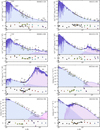 |
Fig. 2 Spectral energy distribution fits to the sample objects (top of each panel) and residuals to the fits (bottom of each panel). The top panels show the SED fits to a DAO (left column) and a DA (right column) WD that do not show an IR excess. The remaining panels (second row: DAO; third and fourth row: DA) depict objects with a near- and/or mid-IR excess modelled with our best fit TMAP models from Paper I and either a best-fit late-type star model from the PHOENIX grid or one or two blackbody component(s). Dots represent observations from different bands, whereas residuals are shown by crosses. Each colour represents a single survey or mission. The dark purple line shows the best-fit (combined) model. Blue and purple areas show the fluxes from the WD and the cool component, respectively. For clarity, the y axis of all panels are shown in the form fλ λ3, except for WD 1342+443, WD 2218+706, and WD 2350–706 where fλ is shown on a logarithmic scale. |
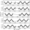 |
Fig. 3 Time-series TESS photometry (grey) of WD 0232+035. Each panel represents a TESS sector. A fit of a harmonic series, as a combination of two significant periods (4.23 and 1.39 d), to the entire TESS dataset is overplotted in black. |
4.2 Kiel masses versus gravity masses
In Paper I, we used the atmospheric parameters measured from our spectroscopic analysis to interpolate masses from the evolutionary tracks of H-rich WDs by Renedo et al. (2010) in the Kiel diagram (MKiel). In Sect. 3 in this paper, we additionally calculated gravity masses (Mgrav = gR2/G) using the log g and R obtained from spectral analysis and SED fitting, respectively. Comparing7 the results of these two methods revealed that gravity and Kiel masses agree within 1 σ for 83% (15/18) of DA and 38% (5/13) of DAO WDs in our sample.
The conspicuous disparity between Kiel and gravity masses, particularly for the DAO WDs, is evident in Fig. 4. This issue manifests systematically as a lower Mgrav compared to MKiel in all cases where a statistical disagreement is identified. It is evident that DAO WDs are more severely affected by this problem than DAs, consistent with the findings of Reindl et al. (2023). We emphasise that unlike Reindl et al. (2023) who report only statistical errors from a metal-free χ2 analysis, our errors also include systematic errors. Despite including systematic errors, the discrepancy between Kiel and gravity masses persists.
We consider Kiel masses to be more reliable than gravity masses. That is because the mean Kiel mass derived in Paper I (⟨MKiel-DAO⟩ = 0.55 M⊙, σ = 0.02 M⊙) is close to the mean Kiel mass of DAs from Paper I (⟨MKiel-DA⟩ = 0.59 M⊙, σ = 0.05 M⊙) and the mean Kiel masses for DAs reported by Gianninas et al. (2010), Bédard et al. (2020), and Reindl et al. (2023). Conversely, the mean gravity mass for DAOs in our sample (Mgrav-DAO⟩ = 0.36 M⊙, σ = 0.12 M⊙) is significantly lower than the mean Kiel masses mentioned above, as well as the mean gravity mass for cool hydrogen-rich WDs (⟨Mgrav⟩ = ![Mathematical equation: $\[0.61_{-0.08}^{+0.14}\]$](/articles/aa/full_html/2026/02/aa57071-25/aa57071-25-eq30.png) M⊙reported by Raddi et al. (2025).
M⊙reported by Raddi et al. (2025).
The discrepancy between the mass determination methods based on theoretical tracks and those based on observed parallaxes is a known problem for hot WDs (Löbling et al. 2020; Reindl et al. 2023). The same issue also appears in other forms. Several studies have reported a mismatch between spectroscopic and parallax distances, with the former generally reported to be larger than the latter (Napiwotzki 2001; Rauch et al. 2007; Ziegler et al. 2012; Reindl et al. 2024). Although in good agreement overall, tests of the theoretical mass–radius relation8 show that the radii and masses of hot WDs derived from parallax measurements and stellar spectroscopy tend to deviate more from theoretical predictions than those of cooler objects (Bédard et al. 2017; Tremblay et al. 2017; Joyce et al. 2018). In all of these studies, the larger uncertainties in the atmospheric parameters are considered to be the source of the observed spread, affecting both hot and cool WDs. Revisiting the results of Bédard et al. (2017), Bergeron et al. (2019) report that, in tests of the theoretical mass–radius relationship, the number of objects lying above the 1σ uncertainty level does not change substantially even after the release of the improved Gaia DR2 parallaxes.
Measuring atmospheric parameters of hot WDs is notoriously difficult because the analysis of their optical spectra is heavily hindered by the Balmer line problem (BLP; see Paper I and references therein). Reindl et al. (2023) argue that quantitative UV spectral analysis using metal line blanketed nonlocal thermodynamic equilibrium model atmospheres could improve the atmospheric parameters and thereby mitigate the mismatch between the masses determined via different methods. Contrary to these expectations, our study does not support this idea, in which we determined Kiel and gravity masses for the largest sample of the hottest WDs to date using the former method. In fact, including metal opacities seems to slightly worsen the discrepancy between Kiel and gravity masses. This is illustrated in Fig. 5, where we compare the gravity masses obtained from the SED fits using our fully metal line blanketed models from Paper I, with those obtained from the SED fits using the metal-free H+He grid from Reindl et al. (2023). The SED fits using the metal-free grid predict radii and gravity masses that are on average 54 and 10% higher, respectively, than those derived from fully metal line blanketed models. This occurs because models that include metals predict slightly higher fluxes from the far-UV to the near-IR compared to pure H+He models. Given the fixed Teff and log g, this leads to a lower angular diameter compared to H+He models and, consequently, lower R and Mgrav for a given observed flux and parallax. However, the differences in radii and gravity masses between the two methods are minor.
Neither photometric variability nor the presence of the IR excess appear to be correlated with the mass inconsistency. We also find no correlation between the mismatch with the values we derived for interstellar reddening (Table A.1). Conversely, a possible correlation may exist between Teff and the occurrence of mass disagreement. While only 15% of the objects with Teff ≤ 70 kK show mass disagreement, this value is 50% for objects above 70 kK. Since log g correlates directly with gravity mass, one might argue that log g values derived in Paper I are systematically underestimated. To test this argument, we increased log g of the sample WDs by 0.3 dex and recalculated the Kiel and gravity masses. However, this approach resulted in unrealistically large gravity masses for 65% of the objects, with differences of up to ~0.8 M⊙ compared to Kiel masses. Although a tighter constraint on log g might mitigate the problem, a systematic error in the log g derivation is unlikely.
In addition to the impact of the results from the quantitative spectral analysis, parallax measurements from the Gaia mission might also influence the observed discrepancy. We find that 27% of objects with a parallax measurement larger than 5 mas show a mismatch between Mgrav and MKiel, while this value is 40% for objects with parallaxes smaller than 5 mas. However, this may simply reflect the fact that the closest objects also tend to be cooler. As parallax increases, it is also unlikely that the mismatch is solely due to the zero-point correction (Reindl et al. 2023). We cannot identify a specific cause for the observed mass disagreement. Most likely, a combination of systematic uncertainties in the observations and in the atmospheric parameters is responsible for the detected inconsistency.
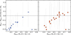 |
Fig. 4 Comparison between gravity and Kiel masses of DAO (blue) and DA (red) WDs. The dashed line represents a 1:1 comparison. Gravity masses were calculated using the radii and surface gravities derived by employing metal line blanketed models in the SED fits and spectral analysis, respectively. |
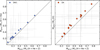 |
Fig. 5 Comparison of gravity masses obtained using metal line blanketed models and pure H and/or H+He models. The dashed line represents a 1:1 comparison. |
4.3 Evolution of He abundance in the Hertzsprung–Russell diagram
We conclude this section by discussing the measured luminosities of our sample WDs. Napiwotzki (1999) reported a decreasing He abundance with decreasing luminosity in their DAO-type CSPNe sample, which they interpreted as indirect evidence for radiation-driven winds. A similar correlation is evident in our sample, as shown in Fig. 6. The decline in He abundance with luminosity is apparent; at L ≈ 300 L⊙, we observe approximately solar He abundance. A sharper decline begins at L ≈ 100 L⊙. The characteristic change in He abundance is consistent with previous studies (Napiwotzki 1999; Unglaub & Bues 2000). Some scatter emerges at L ≈ 65 L⊙, which is expected and occurs because the theoretically predicted termination of mass loss varies with different masses and initial metallicity (Unglaub & Bues 2000), as was also observationally confirmed in Paper I.
Finally, a clear separation of DAO and DA WDs is evident in the Hertzsprung-Russell diagram (HRD; Fig. B.2) consistent with that observed in the Kiel Diagram in Paper I. Our photometric results further reinforce the conclusion of our spectral analysis that all hydrogen-rich WDs are born as DAOs and transform into DA WDs as they cool.
5 Summary and conclusions
We performed a photometric analysis of a sample of 19 DA and 13 DAO WDs with Teff > 60 kK. All sample objects had at least one archival light curve available from TESS, ZTF, CSS, ATLAS, or Gaia. By searching for periodic signals in these datasets, we find that four of the 32 objects in our sample exhibit photometric variability. This corresponds to a variability rate of ![Mathematical equation: $\[13_{-4}^{+8}\]$](/articles/aa/full_html/2026/02/aa57071-25/aa57071-25-eq31.png) %, which agrees with the variability rate reported for H-rich, non-UHE WDs by Reindl et al. (2021). Furthermore, we analysed the SEDs of all WDs in our sample and identified an IR excess in six of 32 sample objects.
%, which agrees with the variability rate reported for H-rich, non-UHE WDs by Reindl et al. (2021). Furthermore, we analysed the SEDs of all WDs in our sample and identified an IR excess in six of 32 sample objects.
For the known close DA+dM binary system WD 0232+035, we report, for the first time, a photometric period of 4.23 d based on the TESS light curve. We find that the phase and amplitude of the 4.23 d photometric variability are consistent with expectations for irradiation of the companion. Moreover, we detect an additional lower-amplitude photometric variability with a period of 1.39 d which is roughly one third of the orbital period. The beating of these two signals produces an unusual light curve shape. The origin of the 1.39 d period remains unclear. We find that WD 1056+516 exhibits a 0.11 d variability in the ZTF g- and r-bands, with similar amplitudes in both bands. We speculate that this variability could be caused by a spot on the surface of the WD, due to the lack of an IR excess. One of the most notable discoveries is the photometric variability of
WD 1342+443, which exhibits similar, low-amplitude variations in the ZTF g- and r-bands with a period of 1.87 d. We have detected, for the first time, weak emission lines in the optical spectra of this object, which strongly suggests that it is an irradiation effect system. Our SED fit suggests that the midIR excess arises from cool dust (≈350 K) that must be located farther from the star. We also demonstrate that any companion with a spectral type earlier than L2.0 would be detectable in the SED, prompting speculation that WD 1342+443 may host an irradiated sub-stellar companion. Future IR and time-resolved spectroscopic observations are required to better characterise the system. For WD 2218+760 we show that the IR excess can be explained by warm (≈560 K) and cold (≈80 K) dust. Finally, we suggest that the 1.37 d period detected in WD 2350–706 likely corresponds to the rotational period of its wide F-type companion.
The SED fitting also yielded radii, luminosities and, in combination with log g from spectroscopy, gravity masses for the WDs. Consequently, the separation of DA and DAO WDs in the Teff –log g plane seen in Paper I is also reproduced in the HRD. In addition, we reinvestigated a longstanding issue in the hottest WDs: the disagreement of Kiel and gravity masses. Specifically, for the first time in a large sample, we assessed if the inclusion of metal opacities in both spectroscopic analysis and SED fitting mitigates this problem. We find that, despite sophisticated metal line blanketed model atmosphere analysis, Kiel and gravity masses agree only in 65% of cases. In particular, for DAO WDs, the gravity masses appear unrealistically low, and, unexpectedly, including metal opacities mildly exacerbates the problem. Although we cannot resolve this problem, we note that this discrepancy worsens with increasing effective temperatures and possibly decreasing parallaxes. We strongly encourage further investigations into this issue.
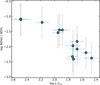 |
Fig. 6 Helium abundance - luminosity relation of the sample DAO WDs. |
Acknowledgements
We thank the referee for a constructive report that helped to improve the paper. We also thank Veronika Schaffenroth, and JJ Hermes for the helpful discussions. S.F. is supported by the Deutsches Zentrum für Luft- und Raumfahrt (DLR) through grant 50 OR 2315. N.R. is supported by the Deutsche Forschungsgemeinschaft (DFG) through grant RE3915/2-1. D.J. acknowledges support from the Agencia Estatal de Investigación del Ministerio de Ciencia, Innovación y Universidades (MCIU/AEI) under grant “Nebulosas planetarias como clave para comprender la evolución de estrellas binarias” and the European Regional Development Fund (ERDF) with reference PID-2022-136653NA-I00 (DOI:10.13039/501100011033). D.J. also acknowledges support from the Agencia Estatal de Investigación del Ministerio de Ciencia, Innovación y Universidades (MCIU/AEI) under grant “Revolucionando el conocimiento de la evolución de estrellas poco masivas” and the European Union NextGenerationEU/PRTR with reference CNS2023-143910 (DOI:10.13039/501100011033). P.S. acknowledges support from the Agencia Estatal de Investigación del Ministerio de Ciencia, Innovación y Universidades (MCIU/AEI) under grant “Revolucionando el conocimiento de la evolución de estrellas poco masivas” and the European Union NextGenerationEU/PRTR with reference CNS2023-143910 (DOI:10.13039/501100011033). M.D. was supported by the Deutsches Zentrum für Luft- und Raumfahrt (DLR) through grant 50-OR-2304. The TMAD (http://astro.uni-tuebingen.de/~TMAD) and TIRO tool (http://astro.uni-tuebingen.de/~TIRO) used for this paper was constructed as part of the activities of the German Astrophysical Virtual Observatory. This work has made use of data from the European Space Agency (ESA) mission Gaia (https://www.cosmos.esa.int/gaia), processed by the Gaia Data Processing and Analysis Consortium (DPAC, https://www.cosmos.esa.int/web/gaia/dpac/consortium). Based on observations obtained with the Samuel Oschin 48-inch Telescope at the Palomar Observatory as part of the Zwicky Transient Facility project. Supported by the National Science Foundation under Grants No. AST-1440341 and AST-2034437 and a collaboration including current partners Caltech, IPAC, the Oskar Klein Center at Stockholm University, the University of Maryland, University of California, Berkeley, the University of Wisconsin at Milwaukee, University of Warwick, Ruhr University, Cornell University, Northwestern University and Drexel University. Operations are conducted by COO, IPAC, and UW. This work includes data from the Asteroid Terrestrial-impact Last Alert System (ATLAS) project. ATLAS is primarily funded to search for near earth asteroids through NASA grants NN12AR55G, 80NSSC18K0284, and 80NSSC18K1575; byproducts of the NEO search include images and catalogs from the survey area. The ATLAS science products have been made possible through the contributions of the University of Hawaii Institute for Astronomy, the Queen’s University Belfast, the Space Telescope Science Institute, and the South African Astronomical Observatory. The CSS survey is funded by the National Aeronautics and Space Administration under Grant No. NNG05GF22G issued through the Science Mission Directorate Near-Earth Objects Observations Program. The CRTS survey is supported by the U.S. National Science Foundation under grants AST0909182 and AST-1313422. The UHS is a partnership between the UK STFC, The University of Hawaii, The University of Arizona, Lockheed Martin and NASA. This paper includes data collected with the TESS mission, obtained from the MAST data archive at the Space Telescope Science Institute (STScI). Funding for the TESS mission is provided by the NASA Explorer Program. STScI is operated by the Association of Universities for Research in Astronomy, Inc., under NASA contract NAS 5-26555. This work made use of tpfplotter by J. Lillo-Box (publicly available in www.github.com/jlillo/tpfplotter), which also made use of the python packages astropy, lightkurve, matplotlib and numpy. This research has made use of NASA’s Astrophysics Data System and the SIMBAD database, operated at CDS, Strasbourg, France. This research has made use of the VizieR catalogue access tool, CDS, Strasbourg, France. This research made use of TOPCAT, an interactive graphical viewer and editor for tabular data (Taylor 2005).
References
- Alam, S., Albareti, F. D., Allende Prieto, C., et al. 2015, ApJS, 219, 12 [Google Scholar]
- Allard, F., Homeier, D., & Freytag, B. 2011, ASP Conf. Ser., 448, 91 [Google Scholar]
- Aller, A., Lillo-Box, J., Jones, D., Miranda, L. F., & Barceló Forteza, S. 2020, A&A, 635, A128 [NASA ADS] [CrossRef] [EDP Sciences] [Google Scholar]
- Aller, A., Lillo-Box, J., & Jones, D. 2024, A&A, 690, A190 [NASA ADS] [CrossRef] [EDP Sciences] [Google Scholar]
- Alonso-García, J., Saito, R. K., Hempel, M., et al. 2018, A&A, 619, A4 [Google Scholar]
- Aungwerojwit, A., Gänsicke, B. T., Rodríguez-Gil, P., et al. 2007, A&A, 469, 297 [NASA ADS] [CrossRef] [EDP Sciences] [Google Scholar]
- Barber, S. D., Belardi, C., Kilic, M., & Gianninas, A. 2016, MNRAS, 459, 1415 [NASA ADS] [CrossRef] [Google Scholar]
- Barnett, J. W., Williams, K. A., Bédard, A., & Bolte, M. 2021, AJ, 162, 162 [NASA ADS] [CrossRef] [Google Scholar]
- Barstow, M. A., Holberg, J. B., Fleming, T. A., et al. 1994, MNRAS, 270, 499 [NASA ADS] [Google Scholar]
- Barstow, M. A., Bond, H. E., Burleigh, M. R., & Holberg, J. B. 2001, MNRAS, 322, 891 [Google Scholar]
- Bédard, A., Bergeron, P., & Fontaine, G. 2017, ApJ, 848, 11 [CrossRef] [Google Scholar]
- Bédard, A., Bergeron, P., Brassard, P., & Fontaine, G. 2020, ApJ, 901, 93 [Google Scholar]
- Bédard, A., Blouin, S., & Cheng, S. 2024, Nature, 627, 286 [CrossRef] [Google Scholar]
- Bellm, E. C., Kulkarni, S. R., Barlow, T., et al. 2019, PASP, 131, 068003 [Google Scholar]
- Benedict, G. F., McArthur, B. E., Franz, O. G., et al. 2000, AJ, 119, 2382 [Google Scholar]
- Bergeron, P., Dufour, P., Fontaine, G., et al. 2019, ApJ, 876, 67 [NASA ADS] [CrossRef] [Google Scholar]
- Bianchi, L., Shiao, B., & Thilker, D. 2017, ApJS, 230, 24 [Google Scholar]
- Bilíková, J., Chu, Y.-H., Gruendl, R. A., Su, K. Y. L., & De Marco, O. 2012, ApJS, 200, 3 [Google Scholar]
- Brinkworth, C. S., Marsh, T. R., Dhillon, V. S., & Knigge, C. 2006, MNRAS, 365, 287 [Google Scholar]
- Brown, J. M., Kilic, M., Brown, W. R., & Kenyon, S. J. 2011, ApJ, 730, 67 [NASA ADS] [CrossRef] [Google Scholar]
- Calcaferro, L. M., Córsico, A. H., Camisassa, M. E., Althaus, L. G., & Shibahashi, H. 2017, EPJ Web Conf., 152, 06012 [Google Scholar]
- Casewell, S. L., Braker, I. P., Parsons, S. G., et al. 2018, MNRAS, 476, 1405 [NASA ADS] [CrossRef] [Google Scholar]
- Casewell, S. L., Debes, J., Braker, I. P., et al. 2020, MNRAS, 499, 5318 [NASA ADS] [CrossRef] [Google Scholar]
- Casewell, S. L., Burleigh, M. R., Napiwotzki, R., et al. 2024, MNRAS, 535, 753 [Google Scholar]
- Chu, Y.-H., Su, K. Y. L., Bilikova, J., et al. 2011, AJ, 142, 75 [NASA ADS] [CrossRef] [Google Scholar]
- Ciardullo, R., Bond, H. E., Sipior, M. S., et al. 1999, AJ, 118, 488 [Google Scholar]
- Cifuentes, C., Caballero, J. A., Cortés-Contreras, M., et al. 2020, A&A, 642, A115 [NASA ADS] [CrossRef] [EDP Sciences] [Google Scholar]
- Clayton, G. C., De Marco, O., Nordhaus, J., et al. 2014, AJ, 147, 142 [NASA ADS] [CrossRef] [Google Scholar]
- Colman, I. L., Angus, R., David, T., et al. 2024, AJ, 167, 189 [Google Scholar]
- Conroy, K. E., Kochoska, A., Hey, D., et al. 2020, ApJS, 250, 34 [Google Scholar]
- Cunningham, T., Tremblay, P.-E., & W. O’Brien, M. 2024, MNRAS, 527, 3602 [Google Scholar]
- De Angeli, F., Weiler, M., Montegriffo, P., et al. 2023, A&A, 674, A2 [NASA ADS] [CrossRef] [EDP Sciences] [Google Scholar]
- De Marco, O., Passy, J.-C., Frew, D. J., Moe, M., & Jacoby, G. H. 2013, MNRAS, 428, 2118 [NASA ADS] [CrossRef] [Google Scholar]
- Drake, A. J., Djorgovski, S. G., Mahabal, A., et al. 2009, ApJ, 696, 870 [Google Scholar]
- Dye, S., Lawrence, A., Read, M. A., et al. 2018, MNRAS, 473, 5113 [Google Scholar]
- El-Badry, K., Rix, H.-W., & Heintz, T. M. 2021, MNRAS, 506, 2269 [NASA ADS] [CrossRef] [Google Scholar]
- Eyer, L., Audard, M., Holl, B., et al. 2023, A&A, 674, A13 [NASA ADS] [CrossRef] [EDP Sciences] [Google Scholar]
- Faedi, F., West, R. G., Burleigh, M. R., Goad, M. R., & Hebb, L. 2011, MNRAS, 410, 899 [NASA ADS] [CrossRef] [Google Scholar]
- Fazio, G. G., Hora, J. L., Allen, L. E., et al. 2004, ApJS, 154, 10 [Google Scholar]
- Filiz, S., Werner, K., Rauch, T., & Reindl, N. 2024, A&A, 691, A290 [NASA ADS] [CrossRef] [EDP Sciences] [Google Scholar]
- Fitzpatrick, E. L., Massa, D., Gordon, K. D., Bohlin, R., & Clayton, G. C. 2019, ApJ, 886, 108 [Google Scholar]
- Flewelling, H. A., Magnier, E. A., Chambers, K. C., et al. 2020, ApJS, 251, 7 [NASA ADS] [CrossRef] [Google Scholar]
- Frew, D. J. 2008, PhD thesis, Macquarie University, Department of Physics and Astronomy, Australia [Google Scholar]
- Frew, D. J., Parker, Q. A., & Bojičić, I. S. 2016, MNRAS, 455, 1459 [Google Scholar]
- Gaia Collaboration 2022, VizieR Online Data Catalog: Gaia DR3 Part 1. Main source (Gaia Collaboration, 2022), VizieR On-line Data Catalog: I/355 [Google Scholar]
- Gaia Collaboration (Brown, A. G. A., et al.) 2016, A&A, 595, A2 [NASA ADS] [CrossRef] [EDP Sciences] [Google Scholar]
- Gaia Collaboration (Brown, A. G. A., et al.) 2018, A&A, 616, A1 [NASA ADS] [CrossRef] [EDP Sciences] [Google Scholar]
- Gaia Collaboration (Brown, A. G. A., et al.) 2021, A&A, 649, A1 [NASA ADS] [CrossRef] [EDP Sciences] [Google Scholar]
- Gaia Collaboration (Vallenari, A., et al.) 2023, A&A, 674, A1 [NASA ADS] [CrossRef] [EDP Sciences] [Google Scholar]
- Gänsicke, B. T., Marsh, T. R., Southworth, J., & Rebassa-Mansergas, A. 2006, Science, 314, 1908 [Google Scholar]
- Genest-Beaulieu, C., & Bergeron, P. 2019, ApJ, 871, 169 [NASA ADS] [CrossRef] [Google Scholar]
- Gentile Fusillo, N. P., Tremblay, P.-E., Gänsicke, B. T., et al. 2019, MNRAS, 482, 4570 [Google Scholar]
- Gentile Fusillo, N. P., Tremblay, P. E., Cukanovaite, E., et al. 2021, MNRAS, 508, 3877 [NASA ADS] [CrossRef] [Google Scholar]
- Gianninas, A., Bergeron, P., Dupuis, J., & Ruiz, M. T. 2010, ApJ, 720, 581 [NASA ADS] [CrossRef] [Google Scholar]
- Gianninas, A., Bergeron, P., & Ruiz, M. T. 2011, ApJ, 743, 138 [Google Scholar]
- Good, S. A., Barstow, M. A., Burleigh, M. R., Dobbie, P. D., & Holberg, J. B. 2005, MNRAS, 364, 1082 [NASA ADS] [CrossRef] [Google Scholar]
- Greenstein, J. L., & Eggen, O. J. 1966, Vistas Astron., 8, 63 [NASA ADS] [CrossRef] [Google Scholar]
- Guo, J., Zhao, J., Tziamtzis, A., et al. 2015, MNRAS, 454, 2787 [NASA ADS] [CrossRef] [Google Scholar]
- Hartman, J. D., & Bakos, G. Á. 2016, Astron. Comp., 17, 1 [Google Scholar]
- Heber, U., Irrgang, A., & Schaffenroth, J. 2018, Open Astron., 27, 35 [Google Scholar]
- Heinze, A. N., Tonry, J. L., Denneau, L., et al. 2018, AJ, 156, 241 [Google Scholar]
- Hermes, J. J., Gänsicke, B. T., Gentile Fusillo, N. P., et al. 2017a, MNRAS, 468, 1946 [NASA ADS] [CrossRef] [Google Scholar]
- Hermes, J. J., Kawaler, S. D., Bischoff-Kim, A., et al. 2017b, ApJ, 835, 277 [Google Scholar]
- Higgins, M. E., & Bell, K. J. 2023, AJ, 165, 141 [NASA ADS] [CrossRef] [Google Scholar]
- Hillwig, T. C., Frew, D. J., Reindl, N., et al. 2017, AJ, 153, 24 [Google Scholar]
- Holberg, J. B., Oswalt, T. D., Sion, E. M., Barstow, M. A., & Burleigh, M. R. 2013, MNRAS, 435, 2077 [Google Scholar]
- Husser, T. O., Wende-von Berg, S., Dreizler, S., et al. 2013, A&A, 553, A6 [NASA ADS] [CrossRef] [EDP Sciences] [Google Scholar]
- Irrgang, A., Geier, S., Heber, U., et al. 2021, A&A, 650, A102 [NASA ADS] [CrossRef] [EDP Sciences] [Google Scholar]
- Jenkins, J. M., Twicken, J. D., McCauliff, S., et al. 2016, SPIE Conf. Ser., 9913, 99133E [Google Scholar]
- Joyce, S. R. G., Barstow, M. A., Casewell, S. L., et al. 2018, MNRAS, 479, 1612 [NASA ADS] [Google Scholar]
- Kawaler, S. D. 1988, ApJ, 334, 220 [Google Scholar]
- Kawka, A., Vennes, S., Dupuis, J., Chayer, P., & Lanz, T. 2008, ApJ, 675, 1518 [Google Scholar]
- Law, N. M., Kulkarni, S. R., Dekany, R. G., et al. 2009, PASP, 121, 1395 [NASA ADS] [CrossRef] [Google Scholar]
- Lenz, P., & Breger, M. 2005, Commun. Asteroseismol., 146, 53 [Google Scholar]
- Lindegren, L., Hernández, J., Bombrun, A., et al. 2018, A&A, 616, A2 [NASA ADS] [CrossRef] [EDP Sciences] [Google Scholar]
- Lindegren, L., Bastian, U., Biermann, M., et al. 2021, A&A, 649, A4 [EDP Sciences] [Google Scholar]
- Löbling, L., Maney, M. A., Rauch, T., et al. 2020, MNRAS, 492, 528 [Google Scholar]
- Lothringer, J. D., & Casewell, S. L. 2020, ApJ, 905, 163 [NASA ADS] [CrossRef] [Google Scholar]
- Maeda, K., & Shibahashi, H. 2014, PASJ, 66, 76 [Google Scholar]
- Marocco, F., Eisenhardt, P. R. M., Fowler, J. W., et al. 2021, ApJS, 253, 8 [Google Scholar]
- Martin, D. C., Fanson, J., Schiminovich, D., et al. 2005, ApJ, 619, L1 [Google Scholar]
- Masci, F. J., Laher, R. R., Rusholme, B., et al. 2019, PASP, 131, 018003 [Google Scholar]
- McMahon, R. G., Banerji, M., Gonzalez, E., et al. 2013, The Messenger, 154, 35 [NASA ADS] [Google Scholar]
- Napiwotzki, R. 1999, A&A, 350, 101 [Google Scholar]
- Napiwotzki, R. 2001, A&A, 367, 973 [NASA ADS] [CrossRef] [EDP Sciences] [Google Scholar]
- Nebot Gómez-Morán, A., Gänsicke, B. T., Schreiber, M. R., et al. 2011, A&A, 536, A43 [NASA ADS] [CrossRef] [EDP Sciences] [Google Scholar]
- Oliveira da Rosa, G., Kepler, S. O., Soethe, L. T. T., Romero, A. D., & Bell, K. J. 2024, ApJ, 974, 314 [Google Scholar]
- Onken, C. A., Wolf, C., Bessell, M. S., et al. 2019, PASA, 36, e033 [Google Scholar]
- Parsons, S. G., Marsh, T. R., Copperwheat, C. M., et al. 2010, MNRAS, 402, 2591 [Google Scholar]
- Press, W. H., Teukolsky, S. A., Vetterling, W. T., & Flannery, B. P. 1992, Numerical Recipes in C. The art of Scientific Computing (Cambridge: Cambridge University Press) [Google Scholar]
- Prša, A., Conroy, K. E., Horvat, M., et al. 2016, ApJS, 227, 29 [Google Scholar]
- Raddi, R., Rebassa-Mansergas, A., Torres, S., et al. 2025, A&A, 695, A131 [NASA ADS] [CrossRef] [EDP Sciences] [Google Scholar]
- Rauch, T., Ziegler, M., Werner, K., et al. 2007, A&A, 470, 317 [NASA ADS] [CrossRef] [EDP Sciences] [Google Scholar]
- Rebassa-Mansergas, A., Xu, S., Raddi, R., et al. 2022, ApJ, 927, L31 [Google Scholar]
- Reindl, N., Bainbridge, M., Przybilla, N., et al. 2019, MNRAS, 482, L93 [Google Scholar]
- Reindl, N., Schaffenroth, V., Filiz, S., et al. 2021, A&A, 647, A184 [NASA ADS] [CrossRef] [EDP Sciences] [Google Scholar]
- Reindl, N., Islami, R., Werner, K., et al. 2023, A&A, 677, A29 [NASA ADS] [CrossRef] [EDP Sciences] [Google Scholar]
- Reindl, N., Bond, H. E., Werner, K., & Zeimann, G. R. 2024, A&A, 690, A366 [NASA ADS] [CrossRef] [EDP Sciences] [Google Scholar]
- Renedo, I., Althaus, L. G., Miller Bertolami, M. M., et al. 2010, ApJ, 717, 183 [Google Scholar]
- Ricker, G. R., Winn, J. N., Vanderspek, R., et al. 2015, J. Astron. Teles. Instrum. Syst., 1, 014003 [Google Scholar]
- Rieke, G. H., Young, E. T., Engelbracht, C. W., et al. 2004, ApJS, 154, 25 [Google Scholar]
- Riello, M., De Angeli, F., Evans, D. W., et al. 2021, A&A, 649, A3 [NASA ADS] [CrossRef] [EDP Sciences] [Google Scholar]
- Santos, A. R. G., Breton, S. N., Mathur, S., & García, R. A. 2021, ApJS, 255, 17 [NASA ADS] [CrossRef] [Google Scholar]
- Schaffenroth, V., Geier, S., Heber, U., et al. 2018, A&A, 614, A77 [NASA ADS] [CrossRef] [EDP Sciences] [Google Scholar]
- Schlafly, E. F., Meisner, A. M., & Green, G. M. 2019, ApJS, 240, 30 [Google Scholar]
- Skrutskie, M. F., Cutri, R. M., Stiening, R., et al. 2006, AJ, 131, 1163 [NASA ADS] [CrossRef] [Google Scholar]
- Steele, P. R., Burleigh, M. R., Dobbie, P. D., & Barstow, M. A. 2007, MNRAS, 382, 1804 [Google Scholar]
- Steele, P. R., Burleigh, M. R., Dobbie, P. D., et al. 2011, MNRAS, 416, 2768 [NASA ADS] [CrossRef] [Google Scholar]
- Steen, M., Hermes, J. J., Guidry, J. A., et al. 2024, ApJ, 967, 166 [NASA ADS] [CrossRef] [Google Scholar]
- Steinmetz, M., Guiglion, G., McMillan, P. J., et al. 2020, AJ, 160, 83 [NASA ADS] [CrossRef] [Google Scholar]
- Taylor, M. B. 2005, ASP Conf. Ser., 347, 29 [Google Scholar]
- Thorstensen, J. R., Charles, P. A., Margon, B., & Bowyer, S. 1978, ApJ, 223, 260 [Google Scholar]
- Tonry, J. L., Denneau, L., Heinze, A. N., et al. 2018, PASP, 130, 064505 [Google Scholar]
- Tremblay, P. E., Gentile-Fusillo, N., Raddi, R., et al. 2017, MNRAS, 465, 2849 [CrossRef] [Google Scholar]
- Tremblay, P. E., Cukanovaite, E., Gentile Fusillo, N. P., Cunningham, T., & Hollands, M. A. 2019, MNRAS, 482, 5222 [Google Scholar]
- Tweedy, R. W., & Kwitter, K. B. 1996, ApJS, 107, 255 [Google Scholar]
- Unglaub, K., & Bues, I. 2000, A&A, 359, 1042 [NASA ADS] [Google Scholar]
- Vennes, S., & Thorstensen, J. R. 1994, AJ, 108, 1881 [Google Scholar]
- Vennes, S., Thorstensen, J. R., Thejll, P., & Shipman, H. L. 1991, ApJ, 372, L37 [Google Scholar]
- Vennes, S., Christian, D. J., & Thorstensen, J. R. 1998, ApJ, 502, 763 [NASA ADS] [CrossRef] [Google Scholar]
- von Hippel, T., Kuchner, M. J., Kilic, M., Mullally, F., & Reach, W. T. 2007, ApJ, 662, 544 [Google Scholar]
- Werner, K., & Dreizler, S. 1999, J. Comput. Appl. Math., 109, 65 [NASA ADS] [CrossRef] [Google Scholar]
- Werner, K., & Herwig, F. 2006, PASP, 118, 183 [Google Scholar]
- Werner, K., Deetjen, J. L., Dreizler, S., et al. 2003, ASP Conf. Ser., 288, 31 [Google Scholar]
- Werner, K., Dreizler, S., & Rauch, T. 2012, Astrophysics Source Code Library [record ascl:1212.015] [Google Scholar]
- Wright, E. L., Eisenhardt, P. R. M., Mainzer, A. K., et al. 2010, AJ, 140, 1868 [Google Scholar]
- Zechmeister, M., & Kürster, M. 2009, A&A, 496, 577 [CrossRef] [EDP Sciences] [Google Scholar]
- Zheng, L.-L., Gu, W.-M., Sun, M., et al. 2022, ApJ, 936, 33 [Google Scholar]
- Ziegler, M., Rauch, T., Werner, K., Köppen, J., & Kruk, J. W. 2012, A&A, 548, A109 [NASA ADS] [CrossRef] [EDP Sciences] [Google Scholar]
Periodicity search for WD 2353+026 resulted in non-detection.
Perhaps the only WD that challenges this convention is PG 1234+482 with Teff ≈ 55 kK. However, the substellar nature of the companion is not confirmed, because the determined spectral type lies on the BD–dM boundary owing to uncertainties in the IR excess (Steele et al. 2007).
WD 0455–282 was excluded from this comparison due to its unusual RUWE value of 8.65, which is not suitable for the single star astrometric solution implemented by Gaia (Lindegren et al. 2018; Gaia Collaboration 2021).
WD 0232+025 was analysed in all mentioned mass–radius studies, whereas WD 2350–706 was only included in the sample of Joyce et al. (2018).
Appendix A Tables
Effective temperatures, surface gravities, radii, luminosities, gravity and Kiel masses, color excesses, Gaia parallaxes and RUWE factors of DAO and DA WDs.
Appendix B Figures
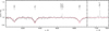 |
Fig. B.1 BOSS spectrum of WD 1342+443 (grey) and the best fit TMAP model (red, Teff = 62 kK and log g = 7.7) from Paper I. |
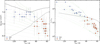 |
Fig. B.2 Sample WDs shown in the Kiel diagram (left) and HRD (right). Solid black line in the left panel corresponds to the theoretical wind limit by (Unglaub & Bues 2000). Dashed black lines in both panels represent predicted He abundance (N(He)/N(H) = 10−3) in the cooling sequence by the same authors, which also matches with the approximate optical detection limit of He. Green dotted lines (left: 0.525, 0.570, 0.593, 0.609, 0.632, 0.659, 0.705, 0.767, and 0.837 M⊙, right: 0.525 - 0.935 M⊙) represent evolutionary tracks of H-rich WDs (Z = 0.01) from Renedo et al. (2010). |
All Tables
Names, spectral types, observed bands, false alarm probabilities, periods, and peak–to–peak amplitudes of the variable objects, as well as the temperatures, radii, and surface ratios of the IR-excess sources.
Effective temperatures, surface gravities, radii, luminosities, gravity and Kiel masses, color excesses, Gaia parallaxes and RUWE factors of DAO and DA WDs.
All Figures
|
Fig. 1 Phase-averaged TESS (orange) and phase-averaged ZTF (green and red) light curves of the variable objects. Peak-to-peak amplitudes were measured by fitting a harmonic series, shown by the black lines. |
| In the text | |
|
Fig. 2 Spectral energy distribution fits to the sample objects (top of each panel) and residuals to the fits (bottom of each panel). The top panels show the SED fits to a DAO (left column) and a DA (right column) WD that do not show an IR excess. The remaining panels (second row: DAO; third and fourth row: DA) depict objects with a near- and/or mid-IR excess modelled with our best fit TMAP models from Paper I and either a best-fit late-type star model from the PHOENIX grid or one or two blackbody component(s). Dots represent observations from different bands, whereas residuals are shown by crosses. Each colour represents a single survey or mission. The dark purple line shows the best-fit (combined) model. Blue and purple areas show the fluxes from the WD and the cool component, respectively. For clarity, the y axis of all panels are shown in the form fλ λ3, except for WD 1342+443, WD 2218+706, and WD 2350–706 where fλ is shown on a logarithmic scale. |
| In the text | |
|
Fig. 3 Time-series TESS photometry (grey) of WD 0232+035. Each panel represents a TESS sector. A fit of a harmonic series, as a combination of two significant periods (4.23 and 1.39 d), to the entire TESS dataset is overplotted in black. |
| In the text | |
|
Fig. 4 Comparison between gravity and Kiel masses of DAO (blue) and DA (red) WDs. The dashed line represents a 1:1 comparison. Gravity masses were calculated using the radii and surface gravities derived by employing metal line blanketed models in the SED fits and spectral analysis, respectively. |
| In the text | |
|
Fig. 5 Comparison of gravity masses obtained using metal line blanketed models and pure H and/or H+He models. The dashed line represents a 1:1 comparison. |
| In the text | |
|
Fig. 6 Helium abundance - luminosity relation of the sample DAO WDs. |
| In the text | |
|
Fig. B.1 BOSS spectrum of WD 1342+443 (grey) and the best fit TMAP model (red, Teff = 62 kK and log g = 7.7) from Paper I. |
| In the text | |
|
Fig. B.2 Sample WDs shown in the Kiel diagram (left) and HRD (right). Solid black line in the left panel corresponds to the theoretical wind limit by (Unglaub & Bues 2000). Dashed black lines in both panels represent predicted He abundance (N(He)/N(H) = 10−3) in the cooling sequence by the same authors, which also matches with the approximate optical detection limit of He. Green dotted lines (left: 0.525, 0.570, 0.593, 0.609, 0.632, 0.659, 0.705, 0.767, and 0.837 M⊙, right: 0.525 - 0.935 M⊙) represent evolutionary tracks of H-rich WDs (Z = 0.01) from Renedo et al. (2010). |
| In the text | |
Current usage metrics show cumulative count of Article Views (full-text article views including HTML views, PDF and ePub downloads, according to the available data) and Abstracts Views on Vision4Press platform.
Data correspond to usage on the plateform after 2015. The current usage metrics is available 48-96 hours after online publication and is updated daily on week days.
Initial download of the metrics may take a while.