| Issue |
A&A
Volume 706, February 2026
|
|
|---|---|---|
| Article Number | A11 | |
| Number of page(s) | 13 | |
| Section | Extragalactic astronomy | |
| DOI | https://doi.org/10.1051/0004-6361/202557213 | |
| Published online | 27 January 2026 | |
Magnetic fields in galactic environments probed by fast radio bursts
1
Instituto de Física, Pontificia Universidad Católica de Valparaíso Casilla 4059 Valparaíso, Chile
2
Department of Astronomy and Astrophysics, University of California, Santa Cruz 1156 High Street Santa Cruz CA 95064, USA
3
Kavli IPMU (WPI), UTIAS, The University of Tokyo Kashiwa Chiba 277-8583, Japan
4
Division of Science, National Astronomical Observatory of Japan 2-21-1 Osawa Mitaka Tokyo 181-8588, Japan
5
Center for Data-Driven Discovery, Kavli IPMU (WPI), UTIAS, The University of Tokyo Kashiwa Chiba 277-8583, Japan
6
Theoretical Astrophysics, Department of Earth & Space Science, Graduate School of Science, The University of Osaka 1-1 Machikaneyama Toyonaka Osaka 560-0043, Japan
7
Theoretical Joint Research, Forefront Research Center, Graduate School of Science, The University of Osaka 1-1 Machikaneyama Toyonaka Osaka 560-0043, Japan
8
Department of Physics & Astronomy, University of Nevada, Las Vegas 4505 S. Maryland Pkwy Las Vegas NV 89154-4002, USA
9
Nevada Center for Astrophysics, University of Nevada, Las Vegas 4505 S. Maryland Pkwy Las Vegas NV 89154-4002, USA
10
Dunlap Institute for Astronomy and Astrophysics, University of Toronto 50 St. George Street Toronto ON M5S 3H4, Canada
11
David A. Dunlap Department of Astronomy and Astrophysics, University of Toronto 50 St. George Street Toronto ON M5S 3H4, Canada
★ Corresponding author: This email address is being protected from spambots. You need JavaScript enabled to view it.
Received:
12
September
2025
Accepted:
20
November
2025
Abstract
Fast radio bursts (FRBs) are extragalactic, bright, millisecond radio pulses emitted by unknown sources. FRBs constitute a unique probe of various astrophysical and cosmological environments via their characteristic dispersion (DM) and Faraday rotation (RM) measures that encode information about the ionised gas traversed by the radio waves along the FRB line of sight. In this work, we analysed the observed RM measured for 14 localised FRBs in the 0.05 ≲ zfrb ≲ 0.5 redshift range, in order to infer the total magnetic field, B, in various galactic environments. Additionally, we calculated fgas – the average fraction of baryons in the ionised CGM. We built a spectroscopic dataset of FRB foreground galaxy halos, acquired with VLT/MUSE observations and by the FLIMFLAM collaboration. We developed a novel Bayesian statistical algorithm and used it to correlate information on the individual intervening halos with the observed RMobs. This approach allowed us to disentangle the magnetic fields present in various environments traversed by the FRB sight lines. Our analysis yields the first direct FRB constraints on the strength of magnetic fields in the interstellar medium (ISM) (Bhostlocal) and in the halos (Bhosthalo) of FRB host galaxies, as well as in the halos of foreground galaxies and groups (Bfghalo). Assuming no field reversals, we find that the average magnetic field strength in the ISM of the FRB host galaxies is Bhostlocal = 5.41.1−0.9μG. Additionally, we placed an upper limit on the average magnetic field strength in FRB host halos, Bhosthalo ≲ 4.8 μG, and in foreground intervening halos, Bfghalo ≲ 4.3 μG. Moreover, we estimated the average fraction of cosmic baryons inside 10 ≲ log10(Mhalo/M⊙) ≲ 13.1 halos to be fgas = 0.45−0.19+0.21. We find that the magnetic field strengths inferred in this work are in good agreement with previous measurements. In contrast to previous studies that analysed FRB RMs and have not considered contributions from the halos of the foreground and/or FRB host galaxies, we show that halos can contribute a non-negligible amount of RM and must be taken into account when analysing future FRB samples.
Key words: galaxies: halos / galaxies: ISM / galaxies: magnetic fields
Simons Pivot Fellow.
© The Authors 2026
 Open Access article, published by EDP Sciences, under the terms of the Creative Commons Attribution License (https://creativecommons.org/licenses/by/4.0), which permits unrestricted use, distribution, and reproduction in any medium, provided the original work is properly cited.
This article is published in open access under the Subscribe to Open model. This email address is being protected from spambots. You need JavaScript enabled to view it. to support open access publication.
1. Introduction
Over the last decades, extragalactic millisecond radio transients, termed fast radio bursts (FRB; Lorimer et al. 2007), have been established as remarkable probes of physical processes spanning a vast range of scales: from atomic to cosmological (e.g. Petroff et al. 2022). While traversing plasma in different cosmic environments, the FRB signal experiences dispersion caused by the free electrons along the propagation path, resulting in a frequency-dependent time delay of the arrival of photons at telescopes on Earth. This characteristic dispersion, referred to as the dispersion measure (DM), has been used extensively to solve the so-called missing baryon problem (McQuinn 2014; Macquart et al. 2020) and to infer how these baryons are distributed in the intergalactic (IGM) and circumgalactic (CGM) media (Simha et al. 2020; Khrykin et al. 2024b; Connor et al. 2025). In addition, analysis of the FRB DM provides a tool for measuring cosmological parameters (e.g., James et al. 2022; Wang et al. 2025; Glowacki & Lee 2024; Fortunato et al. 2025) as well as for assessing galaxy feedback mechanisms (e.g. Khrykin et al. 2024a; Medlock et al. 2025; Zhang et al. 2025; Guo & Lee 2025; Dong et al. 2025; Sharma et al. 2025).
Furthermore, if the propagation medium is magnetised, the intrinsic FRB polarization angle experiences a frequency-dependent rotation, which is characterised by the quantity dubbed the Faraday rotation measure (RM). Akin to the DM, the RM is proportional to the integrated number density of electrons along the propagation path, but additionally weighted by the magnetic field component parallel to the FRB sight line. It therefore offers an opportunity to probe the properties of the magnetic field on different scales in the Universe (Akahori et al. 2016; Kovacs et al. 2024). For instance, observed FRB RMs can be used to constrain the magnetic field generated by the FRB progenitors (e.g. Piro & Gaensler 2018; Lyutikov 2022; Plavin et al. 2022; Anna-Thomas et al. 2023), to refine Milky Way magnetic field constraints (Pandhi et al. 2025), or to shed light on the origin and strength of the magnetic field in the IGM, filaments, and voids of the cosmic web (e.g. Hackstein et al. 2019; Padmanabhan & Loeb 2023; Mtchedlidze et al. 2024).
Measuring the strength of magnetic fields in galaxies is of particular interest, as these are interconnected with the processes of galaxy evolution and feedback (e.g. Bertone et al. 2006; Donnert et al. 2009; Rodrigues et al. 2019). FRBs provide a promising new approach to investigate galactic magnetism, its amplification, and its evolution. For instance, Prochaska et al. (2019) discovered that the FRB 20181112A sight line passes through the halo of a foreground galaxy at bimpact ≃ 29 kpc. Through the analysis of the observed RM, they reported an upper limit on the corresponding parallel component of the magnetic field in the galactic halo of B∥ ≤ 0.8 μG (assuming fiducial halo parameters). This estimate is at odds with previous high-redshift measurements that analysed the RM from a sample of Mg II absorbers at ⟨z⟩ = 1.3 in quasar spectra and found B∥ ≈ 10 μG in the CGM (Bernet et al. 2008). The small B∥ value found by Prochaska et al. (2019) can indicate a little-magnetised halo or a highly disordered magnetic field.
Recently, Mannings et al. (2023) analysed a sample of nine FRBs and reported a positive correlation between DM and extragalactic RMeg given by
 (1)
(1)
with RMobs being the observed RM and RMMW an estimate for the Milky Way contribution. They concluded that the majority of RMeg thus must arise from the host galaxy. Sherman et al. (2023) expanded the sample to 25 FRBs and came to a similar conclusion, emphasising that the bulk of extragalactic RMeg is coming from the ISM of the FRB hosts. However, these works assumed that only FRB progenitors and/or the ISM contribute to the observer RMobs, ignoring any contribution from the halos of the FRB host galaxies. Moreover, they did not account for potential contribution to the observed RMobs from intervening foreground halos. While searching for foreground halos requires extensive spectroscopic observations, ignoring this information can lead to erroneous conclusions (see Lee et al. 2023, for a similar discussion about DMobs in FRB 20190520B).
The goal of this work is to constrain and disentangle the magnetic fields in all galactic environments traversed by the FRB sight lines, including intervening foreground galactic halos. In order to do this, we built a large spectroscopic dataset of galactic halos in the foreground of well-localised FRBs acquired by the FLIMFLAM collaboration (Lee et al. 2022; Simha et al. 2023; Khrykin et al. 2024b; Huang et al. 2025) and dedicated VLT/MUSE observations (PI: N. Tejos). We introduce a novel Bayesian Markov chain Monte Carlo (MCMC) statistical framework that takes into account both observational and modelling uncertainties and recovers the magnetic field strength in various media along the FRB sight lines with high precision levels.
This paper is organised as follows. In Section 2, we outline the main properties of the FRB dataset analysed in this work. We discuss our model for the observed RM and each contributing component in Section 3. We summarise our Bayesian statistical model and present the results of the parameter inference in Section 4. We discuss our findings in Section 5 and conclude in Section 6. Throughout this work, we assumed a flat ΛCDM cosmology with dimensionless Hubble constant h = 0.673, Ωm = 0.315, Ωb = 0.046, σ8 = 0.8, and ns = 0.96, consistent with the latest Planck results (Planck Collaboration VI 2020).
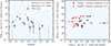 |
Fig. 1. Left: Distribution of absolute values of RMeg as a function of FRB redshift in observer frame. The black dots show the FRB sample analysed in this work, whereas the grey triangles are the DSA-110 subsample taken from Sherman et al. (2023) and the blue diamonds illustrate the FRBs from the Mannings et al. (2023) sample, which are not part of this work. Right: Distribution of RMeg values in rest-frame of FRB hosts as a function of the corresponding |


2. Data sample
In this work, we analysed a sample of 14 FRBs that were detected by the Commensal Real-time ASKAP Fast Transients (CRAFT; Macquart et al. 2010) survey conducted on the Australian Square Kilometre Array Pathfinder (ASKAP) radio telescope. The optical follow-up observations for host identification and redshift measurement were carried out as part of a collaboration between the CRAFT and Fast and Fortunate for FRB Follow-up1 (F4) teams. We built the sample according to the following set of criteria: (1) the posterior probability of FRB-host association by the Probabilistic Association of Transients to their Hosts (PATH; Aggarwal et al. 2021) algorithm must be P(O|x)≥0.90; (2) the FRB must have a publicly available RM measurement; and (3) a given FRB field must have available spectroscopic observations of foreground galaxies. Only 14 FRBs to date satisfy all of the above criteria. We summarise the main properties of the FRBs in the sample in Table 1, noting that the RMobs values adopted here are all taken from Scott et al. (2025).
The left hand panel of Figure 1 shows the estimated extragalactic RMeg, using Eq. (1) and an estimate for RMMW (see Table 1), in our sample as a function of the FRB redshift. Meanwhile, the right hand panel illustrates the distribution of RMeg as a function of the estimated dispersion measure  associated with the host galaxies (halo+ISM/FRB progenitor) of the FRBs in the sample. We also show
  estimates separately via the red markers. The values are adopted from the analysis of Hα flux and halo masses in the FRB hosts by Bernales-Cortes et al. (2025). We ran a Pearson-correlation test between the RMeg and
  and between RMeg and
  values and find no significant correlation in either case with rpearson = 0.10 and rpearson = 0.19, respectively (see also Glowacki et al. 2025).
Sample of 14 FRBs analysed in this work.
We require foreground spectroscopic information in each FRB field in order to identify and characterise galaxies that are intersected by the FRB sight lines in our sample, and that might contribute to the observed RMobs. Recently, the FLIMFLAM survey (Khrykin et al. 2024b; Huang et al. 2025) acquired large spectroscopic samples of galaxies in the foreground of 8 localized FRBs utilised in the FRB foreground-mapping approach (Lee et al. 2022) to infer the distribution of cosmic baryons. For seven of the 14 FRBs in our sample, which are also part of FLIMFLAM DR1 (Khrykin et al. 2024b), we adopted their narrow-field spectroscopic data (within 10″ of the FRB sight lines; see Huang et al. 2025). These observations were performed with the AAOmega spectrograph on the Anglo-Australian Telescope (Smith et al. 2004), the Low-Resolution Imaging Spectrograph (LRIS; Rockosi et al. 2010), the DEep Imaging Multi-Object Spectrograph (DEIMOS; Faber et al. 2003), and the integral field unit (IFU) Keck Cosmic Web Imager (KCWI; Morrissey et al. 2018) on the Keck Telescopes at the W. M. Keck Observatory, and the IFU Multi-Unit Spectroscopic Explorer (MUSE; Bacon et al. 2010) on the Very Large Telescope (VLT). We refer the interested reader to Huang et al. (2025) for more detailed descriptions of these observations. For the remaining 7 FRB fields in our sample lacking FLIMFLAM observations, we used MUSE to obtain the spectra of galaxies within the 1 × 1 arcmin2 field of the respective FRB positions. Each FRB field has been observed for 4 − 8 × 800 s with MUSE to reach r ≲ 25 sources (Bernales-Cortes et al. 2025).
Furthermore, we obtain photometric information on identified foreground galaxies by querying publicly available imaging surveys including the Dark Energy Survey (DES; Abbott et al. 2021), the DECam Local Volume Exploration survey (DELVE; Drlica-Wagner et al. 2022), and the the Panoramic Survey Telescope and Rapid Response System (Pan-STARRS; Chambers et al. 2016). For MUSE sources without data in existing public imaging surveys, we constructed synthetic photometry adopting SDSSg, r, and i filters, but manually setting the transmission to zero beyond the MUSE wavelength range of 4800 − 9300 Å. Additionally, we set the transmission to zero in the 5800 − 5960 Å wavelength window in order to account for the blocking filter used to avoid the light from the laser guide stars. This photometric information is then used to estimate the corresponding stellar masses of identified galaxies via spectral-energy-distribution (SED) fitting. For this purpose, we adopted the publicly available SED-fitting algorithm CIGALE (Boquien et al. 2019) with the initialisation parameters previously used by Simha et al. (2023) and Khrykin et al. (2024b). In what follows, we adopt the mean stellar masses of foreground galaxies estimated by CIGALE and use the average stellar-to-halo mass relation of Moster et al. (2013) to convert to the corresponding halo masses, Mhalo, at a given redshift.
Figure 2 illustrates all halos of galaxies ( ) and groups (
 ) that were observed in the foreground of each FRB in our sample. Those halos that are located at impact parameters bimpact less than equal to their respective virial radii r200 can contribute to the observed RMobs.
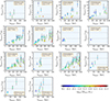 |
Fig. 2. Impact parameter bimpact of identified foreground halos with respect to their virial radius, r200, along each FRB sight line, plotted as a function of the impact parameter. The colour map illustrates the mean mass of the halos, whereas the associated uncertainty is propagated into the error bars on their corresponding r200. The dashed line illustrates the maximum distance, bimpact = r200, at which a foreground halo can be intersected by the FRB sight line and potentially contribute to RMobs if a halo extends to 1 virial radius, r200. In addition, we also show the case where the halos extend to two virial radii, 2 × r200, with the dash-dotted lines. |
3. Rotation measure model
Rotation measure is one of the key observables of the FRB signal. It represents the change in the polarisation angle of the Faraday-rotated polarised emission propagated through the intervening ionised and magnetised gas. While the DM quantifies the integrated number density of free electrons along the propagation path of a signal, the RM describes the same integral, but weighted by the line-of-sight (parallel) component of the magnetic field, B∥:
 (2)
(2)
As an integral quantity, RMobs can be described as a sum of contributions from several components along the FRB line of sight. Thus, for each ith FRB in our sample, we considered the following model for RMobs in the observer frame:
 (3)
(3)
where RMMW, i corresponds to the contribution from the halo and ISM of the Milky Way (see Table 1); RMIGM, i arises from the diffuse gas in the IGM;  is the contribution from the individual, intervening, foreground galactic halos; Nfg is the number of intersected foreground halos; and RMhost, i comes from the FRB host galaxies. In what follows, we discuss each of these components in detail.
3.1. The Milky Way
The contribution from the Milky Way, RMMW, arises both from the magnetised and ionised gas in the Galactic halo and from the ISM within the disk. In this work, we adopted the all-sky Faraday rotation map model from Hutschenreuter et al. (2022) based on ∼55 000 Faraday rotation sources compiled from multiple radio surveys (e.g. LOFAR Two-meter Sky Survey Shimwell et al. 2017 and NRAO VLA Sky Survey Condon et al. 1998 RM catalogue). The map provides a RMMW measurement with associated uncertainty for a given position on the sky. We list the resulting RMMW values for each FRB field in Table 1 (see also Pandhi et al. 2025).
3.2. The intergalactic medium
Due to expected multiple reversals of the intergalactic magnetic field, the RMIGM, arising from the low-density IGM gas tracing the large-scale structure (LSS) of the Universe, is expected to be small relative to other contributing environments (see Eq. 3). The recent LOFAR measurement of ⟨RM⟩≃0.71 ± 0.07 rad m−2 in LSS filaments is consistent with magnetic field of ≃32 nG (e.g. Amaral et al. 2021; Pomakov et al. 2022; Carretti et al. 2022, 2023, and the references within). Given that this RMIGM value is at least 1 − 2 orders of magnitude smaller than the RMobs and RMMW (see Table 1), for the remainder of the paper we assume that the IGM contribution is negligible; i.e. our model adopts
 (4)
(4)
3.3. The foreground halos
In order to estimate the electron density and RM contribution of a given foreground halo intersected by the FRB sight line, we utilised the modified Navarro-Frank-White model (mNFW; Prochaska & Zheng 2019). This model yields a radial density profile ρb(r) of the gas in individual halos given by
 (5)
(5)
where fgas is the fraction of cosmic baryons located in the ionised CGM relative to the total amount of baryons within individual galactic halos; ρ0 is the central density of the halo as a function of halo mass, Mhalo; y ≡ c(r/r200), where c is the concentration parameter; while y0 and α are mNFW model parameters. Here, we adopted the fiducial values y0 = α = 2 from Prochaska & Zheng (2019) while considering fgas as a free parameter. All identified foreground galaxies and groups are illustrated in Figure 2, where we plot the ratio of the halo impact parameter to the corresponding virial radius, r200, as a function of the impact parameter.
The RM contribution of an individual halo in units of rad m−2 is obtained by integrating the density profile ρb(r) given by Eq. (5) as
 (6)
(6)
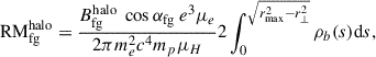
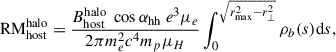
(e.g., Akahori & Ryu 2011), where e and me are the electric charge and mass of the electron, c is the speed of light, mp is the mass of the proton, μH = 1.3 and μe = 1.167 take into account both hydrogen and helium atoms; r⊥ is the impact parameter of the FRB sight line with respect to the centre of the halo, rmax is the maximum extent of the halo in units of r200, and s is the path that the FRB follows inside a given halo. In what follows, we adopted a fixed rmax ≡ r200 value, similarly to the approach of Khrykin et al. (2024b)2. The term  describes the average strength of the total magnetic field in the foreground galactic halos in units of μG, and it is one of the free parameters we considered in this work. In what follows, we assume
  is constant with respect to r. Furthermore,
  is multiplied by the cosine of the angle αfg between the direction of the magnetic field vector and line of sight in order to obtain the required parallel component (see Eq. 3). We note that
  in Eq. (6) is defined in the rest-frame of each foreground halo. We therefore additionally multiplied Eq. (6) by a (1+zhalo)−2 to account for the redshift dilation and convert the result to the observer frame.
In addition, both the stellar mass estimate and the stellar-to-halo mass relation are subjects of considerable uncertainties. Similarly to Khrykin et al. (2024b), we took these uncertainties into account by introducing a random scatter of 0.3 dex to the inferred mass of each halo (see Simha et al. 2021 for more details). For each foreground halo, we constructed a log-normal distribution of its halo mass adopting the corresponding mean and standard deviation values. We then randomly drew N = 1000 realisations of the halo mass from this distribution. Additionally, in order to account for the orientation of the magnetic field, for each draw we randomly chose an angle, αfg, from the uniform distribution 𝒰[0, π] and calculated the corresponding  value given by Eq. (6).
An example of the model distribution of  values for a single foreground halo located bimpact = 150 kpc away from the FRB 20211212A sight line is illustrated by the histogram in the left panel of Figure 3. It is apparent that the
  histogram is centred around RM ≃ 0 rad m−2. In the particular case of this foreground halo, for the majority of the halo mass realisations the extent of the halo, r200, is smaller than the corresponding impact parameter of the halo (bimpact = 150 kpc; see Figure 2). Therefore, in the realisations where the sight line does not actually intersect the foreground halo, the resulting RM
 is effectively zero.
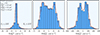 |
Fig. 3. Example of typical distributions of RM values for FRB 20211212A: (left) from the mNFW model of a single foreground galactic halo (see Section 3.3); (middle) from the mNFW model of the corresponding host-galaxy halo (see Section 3.4.1); and (right) from the local environment in the ISM of the host galaxy and/or FRB progenitor (see Section 3.4.2). The positive values of the histograms correspond to the RM values for the case when the line-of-sight component of the magnetic field is aligned with the direction of the FRB sight line (parallel), whereas the negative parts of the histograms, illustrate the case where the line-of-sight component of the magnetic field is directed away from the observer (anti-parallel). The dashed maroon lines show the KDE fit to the resulting RM distributions (see Section 4). Note the different range of RM values in the panels. |
3.4. The FRB host galaxy
The contribution from the FRB host galaxies to the observed RMobs remains highly uncertain. Previous studies analysing the FRB RMs did not have information about the foreground large-scale structures (LSS) and galactic halos, attributing all the extragalactic RM (after subtracting the contribution from the Milky Way) to the FRB hosts. Moreover, some previous works assumed that all of the host contribution arises only from the ISM or local FRB environment, ignoring potential contributions from the extended halo of the host galaxy (e.g. Mannings et al. 2023). In this work, we attempted to explicitly model both the halo and local contributions from the FRB hosts, employing the following model:
 (7)
(7)
where  describes the contribution from the halo of the FRB host galaxy, and
  denotes the contribution from the FRB progenitor itself and/or the ISM environment of the host galaxy, in which the progenitor resides. Here, similarly to the foreground galaxies, we rescaled RMhost to the observer frame by a factor of (1+zhost)−2. In what follows, we describe the calculation of each of these terms separately.
3.4.1. The host halo
In order to estimate the  for a given FRB in our sample, we followed the discussion in Section 3.3 and similarly adopted the mNFW model. We utilised publicly available estimates of the host stellar masses from Gordon et al. (2023) to describe their halo radial density profiles ρb(r). We then obtained the value of the
  by integrating ρb(r) using Eq. (6). However, contrary to the
  case, we assumed that FRB is located inside the disc of the host galaxy and only integrated over the half of the host halo as
 (8)
(8)
where  is the the average strength of the total magnetic field in the halos of the FRB hosts in units of μG, and it is another free parameter considered in this work. Similar to discussion in Section 3.3, we assume
  is constant with respect to location r in the halo. αhh is the angle between the direction of the
  vector and the line of sight.
We took into account the uncertainty in the halo masses by introducing a random 0.3 dex scatter and performed a Monte Carlo sampling (N = 1000 draws) of the corresponding log-normal distribution of the FRB hosts’ halo masses. Similarly to the  calculations in Section 3.3, for each halo mass realisation we drew a value of αhh from the corresponding uniform distribution αhh ∈ 𝒰[0, π] to take into account the orientation of the magnetic field relative to the line of sight. This procedure results in a distribution of
  values for each host in the sample. An example of such a distribution for the halo of the FRB 20211212A host galaxy is illustrated in the middle panel of Figure 3.
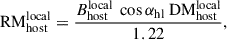
3.4.2. The host ISM/FRB progenitor
To describe the RM associated either with the FRB source itself or with the host galaxy ISM (or both), which we term  , we utilised the RM-DM relation (Akahori et al. 2016; Pandhi et al. 2022), which after accounting for all the constants is given by (in host rest-frame)
 (9)
(9)
where  is the rest-frame dispersion measure in the local FRB environment in units of pc cm−3, the
  is the average strength of the total magnetic field associated with ISM/progenitor in units of μG, and αhl is the angle between the direction of the
  vector and the line of sight. In what follows, we consider
  as another free parameter in our model.
Recently, the analysis of the FLIMFLAM DR1 (Khrykin et al. 2024b; Huang et al. 2025) yielded the first ever published direct estimate of  (DM contribution from the FRB progenitor and/or host ISM), inferring an average contribution of DM
 pc cm−3. We adopted these findings and drew N = 1000 realisations of
  from the corresponding 1D posterior PDF from Khrykin et al. (2024b). Similarly to what is highlighted in the discussion in Sections 3.3 and 3.4.1, we sampled the uniform distribution αhl ∈ 𝒰[0, π] in order to take into account the orientation of the
  vector relative to the FRB sight line. The resulting
  distribution for FRB 20211212A, calculated using Eq. (9), is illustrated by the histogram in the right hand panel of Figure 3.
4. Statistical inference
In order to estimate the set of model parameters 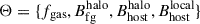 and associated uncertainties, we adopted a Bayesian inference formalism. Therefore, first, we need to define the Bayesian likelihood function ℒFRB(RMobs, i|Θ) for the observed RMobs, i given Θ for each ith FRB in the sample.
4.1. The likelihood function
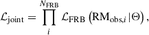
We began by constructing a grid of parameter values on which the likelihood will be estimated. For fgas, we adopted a range of fgas = [0.01, 1.0] with the step Δ = 0.1. Further, we assumed the same range for the strength of the magnetic field in three environments ![Mathematical equation: $ B \equiv B_{\mathrm{fg}}^{\mathrm{halo}} \equiv B_{\mathrm{host}}^{\mathrm{halo}} \equiv B_{\mathrm{host}}^{\mathrm{local}} = [0, 20]\,{\upmu} $](/articles/aa/full_html/2026/02/aa57213-25/aa57213-25-eq56.gif) G with step Δ = 0.5 μG.
G with step Δ = 0.5 μG.
Having defined the parameter grid, we obtain the values of the likelihood function, ℒFRB(RMobs, i|Θ), for a single ith FRB at each point of the parameter grid following the algorithm from Khrykin et al. (2021) as follows.
-
Given the
 and
and  values in Θ, we calculated the corresponding distributions of RM
 and RM
 , respectively (see Sections 3.3 and 3.4.1). Note that for each foreground or FRB host halo, we performed a new random draw from the corresponding uniform distribution describing the orientation angles of a given magnetic field vector. We fitted each of these distributions with a kernel density estimator (KDE; maroon dashed lines in the left hand and middle panels of Figure 3) and then resampled them by randomly drawing N = 2000 realisations of
  and
and  values.
 -
Given the value of
 and assuming the FLIMFLAM estimates of
  we calculated a distribution of RM
 values following Eq. (9). Similarly, to the previous step (1), we fitted the resulting distribution with the KDE (dashed maroon line in the right hand panel of Figure 3) and randomly drew N = 2000 values of
  .
. -
Given the value of RMMW,i and the associated 1σ uncertainty (see Table 1), we constructed a corresponding Gaussian distribution from which we randomly drew N = 2000 realisations of RMMW.
-
We calculated the joint distribution of RMmodel, i values given by Eq. (3) by adding together N = 2000 RM samples obtained through steps (1)–(3). An example of such a joint RMmodel, i distribution for a single realisation of Θ for FRB 20211212A is shown by the histogram in Figure 4.
-
We applied the KDE to the resulting joint RMmodel, i distribution to find its continuous probability-density function (PDF; see dashed maroon line in Figure 4). Finally, we estimated the value of the likelihood function by evaluating the resulting total KDE PDF at the observed value of the RMobs, i for a given FRB (see Table 1 and vertical magenta line in Figure 4).
-
We repeated steps (1)–(5) for each combination of model parameters, Θ.
 |
Fig. 4. Resulting distribution of RMmodel values given by Eq. (3), estimated by combining contributions from each environment along the FRB sight line (see Section 3 and Figure 3 for details). The vertical dashed magenta line illustrates the value of the RMobs for FRB 20211212A, while the horizontal magenta dotted line shows the value of the corresponding log-likelihood value (logℒFRB = −6.41) evaluated from the KDE fit to the RMmodel distribution at the value of RMobs, given the combination of model parameters Θ (see discussion in Section 4 for more details). |
This procedure results in N = NfgasNB3 = 758131 determinations of the likelihood function ℒFRB(RMobs, i|Θ) evaluated on 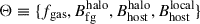 parameter grid for each FRB in the sample. Next, we obtained a joint-likelihood function for the entire sample by taking the product of the individual (independent) likelihood functions:
 (10)
(10)
where NFRB = 14 is the number of FRBs in our sample (see Table 1).
Finally, we interpolated ℒjoint given by Eq. (10) for any arbitrary combination of parameter values that lie between the grid points of the parameter space.
4.2. The priors
As in any Bayesian inference, it is important to be explicit about the adopted priors π on our model parameters, which we define hereafter. First, given the lack of observational information, we adopted a flat, uniform, non-informative prior on the fraction of cosmic baryons in the galactic halos; fgas, i.e., π(fgas) = (0, 1]. Similarly, we used a flat uniform prior for each of the magnetic fields, ![Mathematical equation: $ \pi\left(B_{\mathrm{fg}}^{\mathrm{halo}}\right) = \pi \left(B_{\mathrm{host}}^{\mathrm{halo}}\right) = \pi \left(B_{\mathrm{host}}^{\mathrm{local}}\right) = [0, 20]\,{\upmu} $](/articles/aa/full_html/2026/02/aa57213-25/aa57213-25-eq69.gif) G (e.g. Beck & Wielebinski 2013). Moreover, given the difference in the densities in the halos and the ISM environment of the galaxies, we set the following extra condition:
G (e.g. Beck & Wielebinski 2013). Moreover, given the difference in the densities in the halos and the ISM environment of the galaxies, we set the following extra condition:  (and, analogously,
  ). This is consistent with the expectations from magneto-hydrodynamic simulations (e.g. Ramesh et al. 2023).
In addition, following Khrykin et al. (2024b) we adopted a prior to the total budget of cosmic baryons in the diffuse states outside of the individual galaxies, fd, as
 (11)
(11)
where figm is the fraction of cosmic baryons residing in the diffuse IGM gas, ficm is the fraction of cosmic baryons inside the intracluster medium (ICM) of galaxy clusters with Mhalo ≥ 1014 M⊙, while fcgm is the cosmic baryon fraction in all the halos at Mhalo < 1014 M⊙; in contrast to fgas, which represents the average fraction of the ionised CGM baryons in the individual halos, fcgm represents the fraction of baryons integrated over all CGMs in the Universe. We followed the discussion of Macquart et al. (2020) to estimate fd(z), and we refer the interested reader to the full description provided by Khrykin et al. (2024b). Given the uncertainties in the stellar IMF, evaluating fd(z) at the mean redshift of our FRB sample, ⟨zsample⟩≃0.27, yields fd(z = 0.27)≃0.86 ± 0.02.
In the following, we assumed figm = 0.59 ± 0.10, which is the value found in the FLIMFLAM DR1 analysis by Khrykin et al. (2024b). Following the approach in that work, we calculated the look-up conversion table between fgas and fcgm by integrating the Aemulus halo mass function (McClintock et al. 2019) over the mass range of the halos in our sample, 10 ≲ log10(Mhalo/M⊙)≲13.1 (this includes both foreground and FRB host halos). A similar conversion is adopted between  and ficm assuming Mhalo ≥ 1014 M⊙ and
  , which is consistent with measurements of gas in galaxy clusters (Gonzalez et al. 2013; Chiu et al. 2018).
Additionally, we note that our sample of foreground (see Figure 2) and FRB hosts’ halos does not cover the full range of halo masses below the cluster mass limit of Mhalo ≃ 1014 M⊙. Therefore, we split fcgm into  , representing the halo mass range of our sample, and
  corresponding to the halo mass range of 13.1 ≤ log10(Mhalo/M⊙) < 14.0 not covered by our data. Consequently, at each step of the MCMC inference, the proposed value of fgas is converted to
  using the precomputed lookup table. For the non-cluster halo mass range not covered by our data, we randomly picked a value of fgas for these halos from the uniform distribution 𝒰(0, 1] and converted into the corresponding
  fraction also adopting the Aemulus halo mass function. These terms, together with the mean value of ficm, are then compared to the range of fd(z) in Eq. (11), yielding the following prior:
 (12)
(12)
where σtot takes into account the corresponding uncertainties in fd, figm, and ficm, and is given by
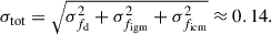 (13)
(13)
4.3. Inference results
Given the expression for the joint-likelihood function described in Section 4.1 and the choice of priors in Section 4.2, we proceeded to sample this ℒjoint. We adopted the publicly available affine-invariant MCMC sampling algorithm EMCEE by Foreman-Mackey et al. (2013) to obtain the posterior probability distributions for our model parameters.
The resulting posterior PDFs of the four model parameters  are illustrated in Figure 5, where the orange (blue) contours correspond to the 68% (95%) confidence intervals (CIs), whereas the marginalised 1D posterior PDFs for each of the model parameters are shown in the diagonal top panels. It is apparent upon inspection of the marginalised posterior PDF that, for some of the considered model parameters, we can only place upper limits, whereas for the others we are able to make a measurement. In order to distinguish between these two cases, we adopted the following criterion. If the peak of the posterior PDF is significantly larger than the posterior PDF values at the edges of the corresponding parameter range, then we classified it as a measurement. We then quoted the median 50th percentile of the marginalised posterior distributions as the measured values, while the corresponding uncertainties are estimated from the 16th and 84th percentiles, respectively. On the other hand, if the above criterion was not met, we reported an upper limit by quoting the 84th percentile (effectively 1σ) of the posterior PDF for a given parameter.
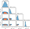 |
Fig. 5. MCMC inference result for sample of 14 FRBs in our dataset (see Table 1). The orange (blue) contours correspond to the inferred 68% (95%) confidence intervals. The diagonal panels show the corresponding marginalised 1D posterior probabilities of the model parameters. |
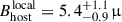
Given our choice of priors in Section 4.2, we estimated the average strength of the magnetic field inside the ISM and/or FRB progenitor to be  G. On the other hand, we were only able to place an upper limit on the average strength of the magnetic field in the FRB host halos because the
  G has a significant posterior probability. Our inference yields
  G. Similarly, we placed an upper limit on the average strength of the magnetic field in foreground halos,
  G. Finally, we inferred the fraction of cosmic baryons inside individual galactic halos to be
  . Following the discussion in Section 4.2 (see Khrykin et al. 2024a, for more details), this implies that a fraction
 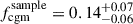 of cosmic baryons reside inside the CGM of the 10 ≲ log10(Mhalo/M⊙) ≲ 13.1 halos.
We present a validation of the accuracy of our inference procedure based on mock FRB experiments in Appendix A, to which we refer the interested reader.
5. Discussion
We now examine how the results of the inference depend on the assumed choice of priors, and discuss our findings in a broader context of previous extragalactic B∥ measurements.
5.1. Effect of the IGM baryon fraction
In our analysis, we explicitly assume that IGM contribution to the RMobs is negligible and do not consider figm as a free parameter in our model (see discussion in Section 3.2). Nevertheless, we needed to adopt a value of figm as part of the prior for our inference algorithm. However, there is a certain degree of degeneracy between figm and fgas, set by the fd(z) prior (see Eq. 11), with the uncertainty due to the fact that the exact partition of the cosmic baryons between the diffuse gas in the IGM and the ionised CGM remains uncertain. Recent FRB studies have produced a mild 1σ tension in the inferred figm fractions. Khrykin et al. (2024b) presented the first results of the FLIMFLAM survey, which utilises a density reconstruction algorithm to constrain the LSS distribution in the foreground of 8 localized FRBs. Their analysis yielded figm = 0.59 ± 0.10, mildly disfavouring strong AGN feedback (Khrykin et al. 2024a). On the other hand, Connor et al. (2025) calibrated the observed DM distribution of 69 localised FRBs (but without information on the foreground halos) to the TNG 300 hydrodynamical simulations. They found 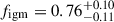 (see also Hussaini et al. 2025), pointing to stronger feedback. In general, this discrepancy in the inferred figm values might affect the accuracy of our inference (i.e. a systematic effect). In order to quantify the significance of the figm constraint on the inference results, we repeated our MCMC analysis described in Section 4, but with different values of the mean figm fraction adopted in the fd(z) prior (see Section 4.2). The resulting 1D marginalised posterior distributions of the model parameters Θ are illustrated in Figure 6, where we show inference results for adopted ⟨figm⟩ = 0.6 (blue), ⟨figm⟩ = 0.8 (orange), and the intermediate case ⟨figm⟩ = 0.7 (green). In addition, we also show the MCMC results without fd(z) prior (red curves).
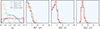 |
Fig. 6. 1D marginalised posterior probability distributions of model parameters considered in this work, estimated with different values of ⟨figm⟩ adopted for the fd(z) prior (see Section 4.2). The fiducial model with ⟨figm⟩ = 0.60 is shown by the blue curves. |
It is apparent from Figure 6, that the choice of ⟨figm⟩ value significantly affects the resulting constraints on fgas. Indeed, for ⟨figm⟩ = 0.8, we estimate fgas ≲ 0.22 ( ), which is at least ≃2 times lower than in our fiducial case with ⟨figm⟩ = 0.6; i.e.
  . This behaviour is expected given the functional form of the fd(z) prior described in Eq. (11), in which figm and fgas are approximately complements of each other. Interestingly, the choice of ⟨figm⟩ does not substantially change the constraints on the
  and
and  , which are illustrated in the middle panels of Figure 6. Both of these quantities are linearly correlated with fgas, given by Eqs. (6) and (8). Nevertheless, we observe that even large changes in ⟨figm⟩ and the correspondingly inferred fgas imply inferences for
  between
  G (⟨figm⟩ = 0.6) and
  G (⟨figm⟩ = 0.8), and that
  and
and  remain mostly unaffected. This is expected given that the magnetic field associated with the ISM of the host galaxy or FRB progenitor does not depend on the diffuse cosmic baryons (see Eq. 9).
According to the results illustrated in Figure 6, improving constraints on figm will be crucial for obtaining the precise measurement on fgas, and therefore for constraining the galactic feedback models (Ayromlou et al. 2023; Khrykin et al. 2024a; Medlock et al. 2024; Connor et al. 2025; Leung et al. 2025). The upcoming FLIMFLAM DR2 (Simha et al., in prep.) will incorporate the analysis of ≈25 localised FRBs with the mapping of foreground structures, which should be enough to bring the figm uncertainty down to the ≈5% level. Additionally, we note that throughout this work we adopted a single fgas parameter to describe the cosmic baryon fraction in all individual halos within a mass range of 10 ≲ log10(Mhalo/M⊙) ≲ 13.1, which our data constrain. However, hydrodynamic simulations indicate that fgas is not only sensitive to the feedback prescriptions, but it is also a function of the halo mass (Khrykin et al. 2024a). The FLIMFLAM-like inference would require NFRB ≃ 300 to distinguish between the fgas fractions in different halo mass bins of the ≈10% level (Huang et al. 2025). The analysis presented in this work suggests that utilizing the RM information alone or in conjunction with FRB DMs and the LSS density reconstructions can dramatically reduce the number of FRBs required to make similar precision predictions on the fgas parameter as a function of halo mass. We will explore this in future work.
In addition, a recent analysis by Zhang et al. (2025) provides an independent estimate of the cosmic baryon fraction in the CGM using the CROCODILE cosmological simulation (Oku & Nagamine 2024) with varying feedback models. They evaluated figm and fcgm through two complementary approaches. First, by directly measuring the CGM mass within halos in their fiducial run, adopting rmax = r200 and a halo mass range of 10.5 ≲ log10(Mhalo/M⊙)≲15.5, they report fcgm ≈ 0.11 − 0.16 at z ≃ 0.28. This total can be broken down into fcgm ≈ 0.07 − 0.08 from halos with log10(Mhalo/M⊙) = [10.5, 13.1] and fcgm ≈ 0.09 from halos with log10(Mhalo/M⊙) = [13.1, 15.5], corresponding to  and
and  in our notation. Notably, despite their lower number density, the more massive halos contribute disproportionately to fcgm, owing to their larger gas reservoirs. Second, they derive a semi-analytic estimate of the statistically averaged intersection fraction using projected density profiles from the simulations. Applying their Eq. (24) yields
  from halos with log10(Mhalo/M⊙) = [10.5, 13.1], and again
  in halos with log10(Mhalo/M⊙) = [13.1, 15.5].
These simulation-based values are somewhat smaller than, though consistent within uncertainties with, our fiducial inference of  for 10 ≲ log10(Mhalo/M⊙)≲13.1 at ⟨z⟩≃0.27 (see Section 4.3). This correspondence between two independent approaches – one with forward modelling of the RM using foreground halo catalogues, and the other direct integration of simulation density profiles – provides a valuable cross-check and highlights the utility of such comparisons for constraining feedback models in the future.
5.2. Magnetic fields in galactic environments at 0.1 ≲ z ≲ 1.0
From our study of 14 FRBs, we found that the average strength of the total magnetic fields in the CGM and ISM/FRB progenitor is B ≲ 6.5 μG. In what follows, we want to place these estimate in the context of previous extragalactic measurements in the late-time Universe. To do this, we converted our results to measurements of B∥ by drawing samples from the MCMC marginalised posterior PDFs and randomly chose the orientation angle of the magnetic field vectors from the corresponding uniform distributions:
![Mathematical equation: $$ \begin{aligned} \begin{aligned}&B_{\parallel ,i} = B_{i} \cos \alpha _{i},\\&B_{i} = \{B_{i,1},\,\ldots ,\,B_{i,N}\} \sim p_{\rm mcmc} \left(\Theta | \mathrm{RM}_{\rm obs}\right),\\&\alpha _{i} = \{\alpha _{i,1},\,\ldots ,\,\alpha _{i,N}\} \overset{i.i.d.}{\sim } \mathcal{U} \left[0,\pi \right], \end{aligned} \end{aligned} $$](/articles/aa/full_html/2026/02/aa57213-25/aa57213-25-eq103.gif) (14)
(14)
where i index denotes a given environment probed by our sample (i.e. foreground halos, halos, and local ISM environment of the FRB hosts). Applying Eq. (14) to the MCMC chains yields ≈4000 realisations of B∥ for each of the magnetic fields we considered in this work. We estimated 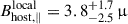 G,
G, 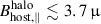 G, and
  G, respectively. Because our inference yielded constraints on the magnetic field strength associated both with the CGM of galaxies and the ISM (and/or FRB progenitors), we compared our results with those of the previous works based on a variety of techniques separately.
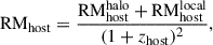
The majority of the CGM constraints come from the analysis of radio-polarisation measurements towards high-z quasars that present strong intervening Mg II absorbers (associated with galactic halos; e.g. Bernet et al. 2008; Farnes et al. 2014; Malik et al. 2020; Burman et al. 2024). Another approach is to correlate the observed RMobs with the distribution of the foreground galaxies (e.g. Lan & Prochaska 2020; Heesen et al. 2023). An alternative method to estimate B∥ is to use FRB sight lines that happen to pass through individual known foreground halos (pioneered by Prochaska et al. 2019) or via the lensing of a source’s polarised emission in the ISM/halo of a foreground galaxy (Mao et al. 2017; Kovacs et al. 2025). Figure 7 presents a compilation of these measurements. It is apparent from the left panel of Figure 7 that our measurements are in good agreement with previous estimates. We note that Prochaska et al. (2019) reported an upper limit that is marginally consistent with our measurement. Moreover, we conclude that foreground or FRB host halos might contribute (on average) a non-negligible amount of RM (thus far usually neglected) and must be taken into account when analysing future observed RMobs of the FRBs.
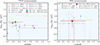 |
Fig. 7. Comparison of B∥ measurements in CGM halos obtained (left panel) and in galactic ISM (right panel), in this (star symbols) and various previous (circles) works. We place |


In the right panel of Figure 7, we compare our  estimate to previous constraints on the magnetic field in the ISM of FRB hosts (Mannings et al. 2023; Sherman et al. 2023) and galaxy discs (Mao et al. 2017). The grey circles show the results obtained by Mannings et al. (2023) from the analysis of eight FRB sight lines. Similarly, the orange circles show the B∥ measurements from the subsample of nine DSA-110 FRBs from Sherman et al. (2023). In addition to plotting the individual measurements, we also calculated and report the average B∥ and a corresponding uncertainty for these two samples, and we illustrate the resulting quantities via the grey and orange triangle markers, respectively. When calculating the average of the Mannings et al. (2023) sample, we excluded the B∥ estimate for FRB 20121102A (|B∥|≃777 ± 366 μG) as a clear outlier, most likely dominated by the immediate environment to the FRB. The average redshift values of Mannings et al. (2023) and Sherman et al. (2023) samples are ⟨z⟩ = 0.2023 and ⟨z⟩ = 0.2739, respectively, whereas ours is ⟨z⟩ = 0.2732. We therefore artificially shifted the corresponding orange triangle by Δz = 0.035 in the figure for the sake of clarity. Finally, we also show the results of the RM analysis of the individual lensed galaxy from Mao et al. (2017). Upon inspection of the right panel of Figure 7, it is apparent that we find B∥ values comparable with the average estimates from previous works. We note, however, that both of the previous works that analysed FRB RMs did not have information about the foreground halos and attributed all the RMeg to the contribution from the local environment in the FRB host galaxies. The fact that
  ,
,  , and
, and  are all of the same order of magnitude implies that all these components must be taken into account in the RMobs.
We remind the reader that our inferences are by construction average B (or average B∥), and thus deviations from these are expected for individual cases. Based on this reasoning, a possible explanation for the apparent peak in B∥ at z ∼ 0.2 (see Figure 1) seen in the combined samples of Mannings et al. (2023) and Sherman et al. (2023) could most likely be attributed to individual excesses of  rather than
  given that much larger density variations are expected (due to geometrical effects). Moreover, within the
  contributions of the ISM and/or local environment of the FRBs, we deem the latter to be the most likely to be responsible for outliers (including the possible peak at z ∼ 0.2). This hypothesis can be tested with an analysis of magnetic fields from larger samples of FRBs. Additional constraints on
  will also be paramount for establishing the origin of the FRB phenomenon.
Finally, we note that our analysis is agnostic with regard to magnetic field reversals in different galactic environments traversed by the FRB sight lines. While this effectively assumes the uniformity of magnetic fields at different galactic scales, given the current limited data sample we opted not to explicitly model it. A more realistic scenario of entangled fields would result in a factor of  amplification of the inferred B values, where N is the number of reversals in a given medium. We leave a more refined consideration of magnetic field correlation lengths and field reversals to future work.
6. Conclusions
We analysed a sample of RMs from Nfrb = 14 FRBs in the 0.05 ≲ zfrb ≲ 0.5 redshift range and correlated it with spectroscopic information about the foreground galactic halos, intersected by the FRB sight lines. We developed a novel Bayesian inference formalism that allows the inferring of the total strength of the magnetic fields present in various galactic environments traversed by the FRB sight lines. The main results of our work are summarised as listed below.
-
For the first time, we successfully disentangled and measured the magnetic field both in the halos and ISM/progenitor environment of the FRB host galaxies. Given our fiducial set of priors, we estimate that, on average, the strength of the magnetic field in the FRB host ISM and/or the FRB progenitor is
 G, whereas we place an upper limit on the magnetic field associated with the FRB host halos
  G.
G. -
In addition, we estimate an upper limit on the magnetic field in the halos of the foreground galaxies and groups; our analysis yielded
 G, which is comparable to the value estimated for the halos of the FRB host galaxies. We note that for a current dataset we cannot exclude the possibility of
  G or
G or  G on a 2σ level.
 -
We find that our constraints are in good agreement with previous estimates of the strength of the parallel component of the magnetic field in the CGM of galaxies, as well as in the ISM environment. We stress that future attempts to measure the magnetic field using FRBs must consider the contribution from the foreground halos.
-
Adopting the mNFW model to describe the radial density profile of the halos of both foreground and FRB host galaxies, we estimated the average fraction of halo baryons inside the ionised CGM of individual galaxies to be
 . This corresponds to the fraction of cosmic baryons
  inside the 10.0 ≲ log10(Mhalo/M⊙)≲13.1 halos.
 -
Our estimates for magnetic fields in the halos of foreground and FRB host galaxies, as well as in the host ISM and/or FRB progenitor environment, are largely unaffected by the average figm value adopted in the fd(z) prior (see Section 4.2). On the other hand, the constraint on fgas is degenerate with the figm measurement (see discussion in Section 5.1).
The results of this work emphasise the significance of the spectroscopic information regarding the foreground structures traversed by the FRB for placing accurate constraints on both cosmological and astrophysical parameters. Multiplex instruments such as MUSE (Bacon et al. 2010), 4MOST (de Jong et al. 2019), and DESI (Levi et al. 2013) will play a crucial role in interpreting DM and RM information from a surging number of FRB detections owing to increasing capabilities of the ASKAP/CRAFT (Macquart et al. 2010; Shannon et al. 2025), CHIME/VLBI (Andrew et al. 2025), CHIME/FRB Outriggers (Lanman et al. 2024; CHIME/FRB Collaboration 2025), and MeerKAT TRAnsients and Pulsars (MeerTrap; Sanidas et al. 2018; Rajwade et al. 2024), as well as, DSA-110 (Ravi et al. 2023) and commissioning of the DSA-2000 (Hallinan et al. 2019). These new data will allow the probing and characterisation of the properties of the magnetic fields in and out of galaxies up to redshift z ∼ 1 and beyond.
Acknowledgments
We are grateful to the anonymous referee for comments and suggestions, which helped us to improve the manuscript. We thank Joscha Jahns-Schindler and members of the Fast and Fortunate for FRB Follow-up collaboration for useful discussion and comments. I.S.K. and N.T. acknowledge support from grant ANID/FONDO ALMA 2024/31240053. N.T. acknowledges support by FONDECYT grant 1252229. KN acknowledge support from MEXT/JSPS KAKENHI Grant Numbers JP19H05810, JP20H00180, and JP22K21349. Kavli IPMU was established by World Premier International Research Center Initiatives (WPI), MEXT, Japan. This work was performed in part at the Center for Data-Driven Discovery, Kavli IPMU (WPI).
References
- Abbott, T. M. C., Adamów, M., Aguena, M., et al. 2021, ApJS, 255, 20 [NASA ADS] [CrossRef] [Google Scholar]
- Aggarwal, K., Budavári, T., Deller, A. T., et al. 2021, ApJ, 911, 95 [NASA ADS] [CrossRef] [Google Scholar]
- Akahori, T., & Ryu, D. 2011, ApJ, 738, 134 [NASA ADS] [CrossRef] [Google Scholar]
- Akahori, T., Ryu, D., & Gaensler, B. M. 2016, ApJ, 824, 105 [NASA ADS] [CrossRef] [Google Scholar]
- Amaral, A. D., Vernstrom, T., & Gaensler, B. M. 2021, MNRAS, 503, 2913 [NASA ADS] [CrossRef] [Google Scholar]
- Andrew, S., Leung, C., Li, A., et al. 2025, ApJ, 981, 39 [Google Scholar]
- Anna-Thomas, R., Connor, L., Dai, S., et al. 2023, Science, 380, 599 [NASA ADS] [CrossRef] [Google Scholar]
- Ayromlou, M., Nelson, D., & Pillepich, A. 2023, MNRAS, 524, 5391 [CrossRef] [Google Scholar]
- Bacon, R., Accardo, M., Adjali, L., et al. 2010, SPIE Conf. Ser., 7735, 773508 [Google Scholar]
- Bannister, K. W., Deller, A. T., Phillips, C., et al. 2019, Science, 365, 565 [NASA ADS] [CrossRef] [Google Scholar]
- Beck, R., & Wielebinski, R. 2013, in Planets, Stars and Stellar Systems. Volume 5: Galactic Structure and Stellar Populations, eds. T. D. Oswalt, & G. Gilmore, 5, 641 [NASA ADS] [Google Scholar]
- Bernales-Cortes, L., Tejos, N., Prochaska, J. X., et al. 2025, A&A, 696, A81 [NASA ADS] [CrossRef] [EDP Sciences] [Google Scholar]
- Bernet, M. L., Miniati, F., Lilly, S. J., Kronberg, P. P., & Dessauges-Zavadsky, M. 2008, Nature, 454, 302 [NASA ADS] [CrossRef] [Google Scholar]
- Bertone, S., Vogt, C., & Enßlin, T. 2006, MNRAS, 370, 319 [NASA ADS] [Google Scholar]
- Bhandari, S., Sadler, E. M., Prochaska, J. X., et al. 2020, ApJ, 895, L37 [NASA ADS] [CrossRef] [Google Scholar]
- Boquien, M., Burgarella, D., Roehlly, Y., et al. 2019, A&A, 622, A103 [NASA ADS] [CrossRef] [EDP Sciences] [Google Scholar]
- Burman, S., Sharma, P., Malik, S., & Singh, S. 2024, JCAP, 2024, 063 [Google Scholar]
- Carretti, E., Vacca, V., O’Sullivan, S. P., et al. 2022, MNRAS, 512, 945 [NASA ADS] [CrossRef] [Google Scholar]
- Carretti, E., O’Sullivan, S. P., Vacca, V., et al. 2023, MNRAS, 518, 2273 [Google Scholar]
- Chambers, K. C., Magnier, E. A., Metcalfe, N., et al. 2016, ArXiv e-prints [arXiv:1612.05560] [Google Scholar]
- CHIME/FRB Collaboration (Amiri, M., et al.) 2025, ApJ, 993, 55 [Google Scholar]
- Chiu, I., Mohr, J. J., McDonald, M., et al. 2018, MNRAS, 478, 3072 [Google Scholar]
- Condon, J. J., Cotton, W. D., Greisen, E. W., et al. 1998, AJ, 115, 1693 [Google Scholar]
- Connor, L., Ravi, V., Sharma, K., et al. 2025, Nat. Astron., 9, 1226 [Google Scholar]
- de Jong, R. S., Agertz, O., Berbel, A. A., et al. 2019, The Messenger, 175, 3 [NASA ADS] [Google Scholar]
- Dong, C., Dedieu, F., Galárraga-Espinosa, D., et al. 2025, ArXiv e-prints [arXiv:2507.16115] [Google Scholar]
- Donnert, J., Dolag, K., Lesch, H., & Müller, E. 2009, MNRAS, 392, 1008 [NASA ADS] [CrossRef] [Google Scholar]
- Drlica-Wagner, A., Ferguson, P. S., Adamów, M., et al. 2022, ApJS, 261, 38 [NASA ADS] [CrossRef] [Google Scholar]
- Faber, S. M., Phillips, A. C., Kibrick, R. I., et al. 2003, SPIE Conf. Ser., 4841, 1657 [Google Scholar]
- Farnes, J. S., O’Sullivan, S. P., Corrigan, M. E., & Gaensler, B. M. 2014, ApJ, 795, 63 [NASA ADS] [CrossRef] [Google Scholar]
- Foreman-Mackey, D., Hogg, D. W., Lang, D., & Goodman, J. 2013, PASP, 125, 306 [Google Scholar]
- Fortunato, J. A. S., Bacon, D. J., Hipólito-Ricaldi, W. S., & Wands, D. 2025, JCAP, 2025, 018 [Google Scholar]
- Glowacki, M., & Lee, K. G. 2024, ArXiv e-prints [arXiv:2410.24072] [Google Scholar]
- Glowacki, M., Bera, A., James, C. W., et al. 2025, ArXiv e-prints [arXiv:2506.23403] [Google Scholar]
- Gonzalez, A. H., Sivanandam, S., Zabludoff, A. I., & Zaritsky, D. 2013, ApJ, 778, 14 [Google Scholar]
- Gordon, A. C., Fong, W.-F., Kilpatrick, C. D., et al. 2023, ApJ, 954, 80 [NASA ADS] [CrossRef] [Google Scholar]
- Guo, Q., & Lee, K.-G. 2025, MNRAS, 540, 289 [Google Scholar]
- Hackstein, S., Brüggen, M., Vazza, F., Gaensler, B. M., & Heesen, V. 2019, MNRAS, 488, 4220 [NASA ADS] [CrossRef] [Google Scholar]
- Hallinan, G., Ravi, V., Weinreb, S., et al. 2019, BAAS, 51, 255 [NASA ADS] [Google Scholar]
- Heesen, V., O’Sullivan, S. P., Brüggen, M., et al. 2023, A&A, 670, L23 [NASA ADS] [CrossRef] [EDP Sciences] [Google Scholar]
- Heintz, K. E., Prochaska, J. X., Simha, S., et al. 2020, ApJ, 903, 152 [NASA ADS] [CrossRef] [Google Scholar]
- Huang, Y., Simha, S., Khrykin, I. S., et al. 2025, ApJS, 277, 64 [Google Scholar]
- Hussaini, M., Connor, L., Konietzka, R. M., et al. 2025, ApJ, 993, L27 [Google Scholar]
- Hutschenreuter, S., Anderson, C. S., Betti, S., et al. 2022, A&A, 657, A43 [NASA ADS] [CrossRef] [EDP Sciences] [Google Scholar]
- James, C. W., Ghosh, E. M., Prochaska, J. X., et al. 2022, MNRAS, 516, 4862 [NASA ADS] [CrossRef] [Google Scholar]
- Khrykin, I. S., Hennawi, J. F., Worseck, G., & Davies, F. B. 2021, MNRAS, 505, 649 [CrossRef] [Google Scholar]
- Khrykin, I. S., Sorini, D., Lee, K.-G., & Davé, R. 2024a, MNRAS, 529, 537 [NASA ADS] [CrossRef] [Google Scholar]
- Khrykin, I. S., Ata, M., Lee, K.-G., et al. 2024b, ApJ, 973, 151 [Google Scholar]
- Kovacs, T. O., Mao, S. A., Basu, A., et al. 2024, A&A, 690, A47 [NASA ADS] [CrossRef] [EDP Sciences] [Google Scholar]
- Kovacs, T. O., Mao, S. A., Basu, A., Ma, Y. K., & Gaensler, B. M. 2025, ArXiv e-prints [arXiv:2507.12542] [Google Scholar]
- Lan, T.-W., & Prochaska, J. X. 2020, MNRAS, 496, 3142 [CrossRef] [Google Scholar]
- Lanman, A. E., Andrew, S., Lazda, M., et al. 2024, AJ, 168, 87 [Google Scholar]
- Lee, K.-G., Ata, M., Khrykin, I. S., et al. 2022, ApJ, 928, 9 [NASA ADS] [CrossRef] [Google Scholar]
- Lee, K.-G., Khrykin, I. S., Simha, S., et al. 2023, ApJ, 954, L7 [NASA ADS] [CrossRef] [Google Scholar]
- Leung, C., Simha, S., Medlock, I., et al. 2025, ApJ, 991, L25 [Google Scholar]
- Levi, M., Bebek, C., Beers, T., et al. 2013, ArXiv e-prints [arXiv:1308.0847] [Google Scholar]
- Lorimer, D. R., Bailes, M., McLaughlin, M. A., Narkevic, D. J., & Crawford, F. 2007, Science, 318, 777 [Google Scholar]
- Lyutikov, M. 2022, ApJ, 933, L6 [NASA ADS] [CrossRef] [Google Scholar]
- Macquart, J.-P., Bailes, M., Bhat, N. D. R., et al. 2010, PASA, 27, 272 [NASA ADS] [CrossRef] [Google Scholar]
- Macquart, J. P., Prochaska, J. X., McQuinn, M., et al. 2020, Nature, 581, 391 [Google Scholar]
- Malik, S., Chand, H., & Seshadri, T. R. 2020, ApJ, 890, 132 [NASA ADS] [CrossRef] [Google Scholar]
- Mannings, A. G., Pakmor, R., Prochaska, J. X., et al. 2023, ApJ, 954, 179 [NASA ADS] [CrossRef] [Google Scholar]
- Mao, S. A., Carilli, C., Gaensler, B. M., et al. 2017, Nat. Astron., 1, 621 [NASA ADS] [CrossRef] [Google Scholar]
- McClintock, T., Rozo, E., Becker, M. R., et al. 2019, ApJ, 872, 53 [NASA ADS] [CrossRef] [Google Scholar]
- McQuinn, M. 2014, ApJ, 780, L33 [Google Scholar]
- Medlock, I., Nagai, D., Singh, P., et al. 2024, ApJ, 967, 32 [Google Scholar]
- Medlock, I., Nagai, D., Anglés-Alcázar, D., & Gebhardt, M. 2025, ApJ, 983, 46 [Google Scholar]
- Morrissey, P., Matuszewski, M., Martin, D. C., et al. 2018, ApJ, 864, 93 [Google Scholar]
- Moster, B. P., Naab, T., & White, S. D. M. 2013, MNRAS, 428, 3121 [Google Scholar]
- Mtchedlidze, S., Domínguez-Fernández, P., Du, X., et al. 2024, ApJ, 977, 128 [NASA ADS] [Google Scholar]
- Oku, Y., & Nagamine, K. 2024, ApJ, 975, 183 [Google Scholar]
- Padmanabhan, H., & Loeb, A. 2023, ApJ, 946, L18 [CrossRef] [Google Scholar]
- Pandhi, A., Hutschenreuter, S., West, J. L., Gaensler, B. M., & Stock, A. 2022, MNRAS, 516, 4739 [NASA ADS] [CrossRef] [Google Scholar]
- Pandhi, A., Gaensler, B. M., Pleunis, Z., et al. 2025, ApJ, 982, 146 [Google Scholar]
- Petroff, E., Hessels, J. W. T., & Lorimer, D. R. 2022, A&ARv, 30, 2 [NASA ADS] [CrossRef] [Google Scholar]
- Piro, A. L., & Gaensler, B. M. 2018, ApJ, 861, 150 [NASA ADS] [CrossRef] [Google Scholar]
- Planck Collaboration VI. 2020, A&A, 641, A6 [NASA ADS] [CrossRef] [EDP Sciences] [Google Scholar]
- Plavin, A., Paragi, Z., Marcote, B., et al. 2022, MNRAS, 511, 6033 [NASA ADS] [CrossRef] [Google Scholar]
- Pomakov, V. P., O’Sullivan, S. P., Brüggen, M., et al. 2022, MNRAS, 515, 256 [NASA ADS] [CrossRef] [Google Scholar]
- Prochaska, J. X., & Zheng, Y. 2019, MNRAS, 485, 648 [NASA ADS] [Google Scholar]
- Prochaska, J. X., Macquart, J.-P., McQuinn, M., et al. 2019, Science, 366, 231 [NASA ADS] [CrossRef] [Google Scholar]
- Rajwade, K. M., Driessen, L. N., Barr, E. D., et al. 2024, MNRAS, 532, 3881 [Google Scholar]
- Ramesh, R., Nelson, D., Heesen, V., & Brüggen, M. 2023, MNRAS, 526, 5483 [NASA ADS] [CrossRef] [Google Scholar]
- Ravi, V., Catha, M., Chen, G., et al. 2023, ApJ, 949, L3 [NASA ADS] [CrossRef] [Google Scholar]
- Rockosi, C., Stover, R., Kibrick, R., et al. 2010, SPIE Conf. Ser., 7735, 77350R [Google Scholar]
- Rodrigues, L. F. S., Chamandy, L., Shukurov, A., Baugh, C. M., & Taylor, A. R. 2019, MNRAS, 483, 2424 [NASA ADS] [CrossRef] [Google Scholar]
- Sanidas, S., Caleb, M., Driessen, L., et al. 2018, in Pulsar Astrophysics the Next Fifty Years, eds. P. Weltevrede, B. B. P. Perera, L. L. Preston, & S. Sanidas, 337, 406 [NASA ADS] [Google Scholar]
- Scott, D. R., Dial, T., Bera, A., et al. 2025, PASA, 42, e133 [Google Scholar]
- Shannon, R. M., Bannister, K. W., Bera, A., et al. 2025, PASA, 42, e036 [Google Scholar]
- Sharma, K., Krause, E., Ravi, V., et al. 2025, ApJ, 989, 81 [Google Scholar]
- Sherman, M. B., Connor, L., Ravi, V., et al. 2023, ApJ, 957, L8 [NASA ADS] [CrossRef] [Google Scholar]
- Shimwell, T. W., Röttgering, H. J. A., Best, P. N., et al. 2017, A&A, 598, A104 [NASA ADS] [CrossRef] [EDP Sciences] [Google Scholar]
- Simha, S., Burchett, J. N., Prochaska, J. X., et al. 2020, ApJ, 901, 134 [NASA ADS] [CrossRef] [Google Scholar]
- Simha, S., Tejos, N., Prochaska, J. X., et al. 2021, ApJ, 921, 134 [NASA ADS] [CrossRef] [Google Scholar]
- Simha, S., Lee, K.-G., Prochaska, J. X., et al. 2023, ApJ, 954, 71 [NASA ADS] [CrossRef] [Google Scholar]
- Smith, G. A., Saunders, W., Bridges, T., et al. 2004, SPIE Conf. Ser., 5492, 410 [Google Scholar]
- Wang, Y.-Y., Gao, S.-J., & Fan, Y.-Z. 2025, ApJ, 981, 9 [Google Scholar]
- Zhang, Z. J., Nagamine, K., Oku, Y., et al. 2025, ApJ, 993, 162 [Google Scholar]
In principle, rmax should also be included as another free parameter (see Prochaska & Zheng 2019; Simha et al. 2020; Lee et al. 2023). However, we tested the model using rmax = 2 × r200 and did not find significant differences in the results. Therefore, in this work, we adopted a fixed truncation radius and will explore a more sophisticated parametrisation in the future.
Appendix A: Inference test on the mock datasets
In order to test the accuracy of our inference algorithm described in Section 4, we apply it to the mock FRB sample. In what follows, we briefly outline the algorithm to generate mock FRB samples and the inference results.
Inference test results for different combinations of the input true model parameters Θ.
First, we randomly draw redshifts for N = 14 mock FRB host galaxies from the corresponding uniform distribution 𝒰[zmin,zmax], where the redshift range is defined to be similar to that of our dataset in Table 1. Second, for each mock FRB galaxy in the sample we assign halo masses by sampling the corresponding uniform distribution ![Mathematical equation: $ \mathcal{U}\left[ M_{\mathrm{halo}}^{\mathrm{min}}, M_{\mathrm{halo}}^{\mathrm{max}}\right] $](/articles/aa/full_html/2026/02/aa57213-25/aa57213-25-eq129.gif) , where the halo mass range is given by the minimum and maximum halo masses in the dataset. Finally, for each mock FRB we create catalogues of the foreground halos. We begin by assigning the number of foreground halos per sightline. To do so we sample the uniform distribution
, where the halo mass range is given by the minimum and maximum halo masses in the dataset. Finally, for each mock FRB we create catalogues of the foreground halos. We begin by assigning the number of foreground halos per sightline. To do so we sample the uniform distribution ![Mathematical equation: $ \mathcal{U}\left[N_{\mathrm{fg}}^{\mathrm{min}}, N_{\mathrm{fg}}^{\mathrm{max}}\right] $](/articles/aa/full_html/2026/02/aa57213-25/aa57213-25-eq130.gif) , where
, where  and
and  are given by the number of foreground halos per sightline in the dataset (see Figure 2). Then, each ith foreground halo along the jth FRB sightline is assigned a redshift
  , impact parameter from the FRB sightline
  , and halo mass
![Mathematical equation: $$ \begin{aligned}&\{z^j\} = \{z_{i = 1}^{j}, .., z_{i=N_{\rm fg}}^{j}\} \overset{i.i.d.}{\sim } \mathcal{U} \left[0, z_{\rm FRB}^{j}\right],\nonumber \\&\{b^j\} = \{b_{i = 1}^{j}, .., b_{i=N_{\rm fg}}^{j}\} \overset{i.i.d.}{\sim } \mathcal{U} \left[30, 3000\right]\,\mathrm{kpc},\nonumber \\&\{M_{\rm halos}^j\} = \{M_{\rm halo,{i = 1}}^{j}, .., M_{\rm halo,i=N_{\rm fg}}^{j}\} \overset{i.i.d.}{\sim } \mathcal{U} \left[10^{10}, 10^{13.1}\right]\,M_{\odot }, \end{aligned} $$](/articles/aa/full_html/2026/02/aa57213-25/aa57213-25-eq136.gif) (A.1)
(A.1)
where the boundaries of the intervals on which the uniform distributions are defined, are chosen to represent the observed dataset. We then assume a set of true model parameters  , and estimate the corresponding mock RMobs given by eq. (3) for each mock FRB sightline. We also include an observational uncertainty by randomly sampling the Gaussian with σ = 2 rad m−2 and adding this error to the resulting mock RMobs values.
Utilizing the catalogues of the foreground halos, and RMobs of each mock FRB in the sample, we then proceed to calculate the joint likelihood of the mock sample, following the discussion in Section 4.1, and sample it with the MCMC algorithm. The resulting posterior PDFs are illustrated in Figure A.1, where the orange (blue) contours correspond to the 68% (95%) confidence intervals (CI), whereas the marginalized posterior PDFs for each of the model parameters are shown in the diagonal panels. The true values of the model parameters are illustrated by the dots in each panel of Figure A.1. Similar to the discussion in Section 4.3, if the maximum of a given 1D marginalized posterior PDF is at least four times larger than the larger of the two posterior PDF values at the edges of the corresponding parameter range, then we quote the 50th percentile of the marginalized posterior distributions as the measured values, while the corresponding uncertainties are estimated from the 16th and 84th percentiles, respectively. On the other hand, if the above criterion is not met, we report an upper limit by quoting the 84th percentile of the posterior PDF for a given parameter.
It is apparent from the inference results in Figure A.1, that our algorithm successfully recovers the input true values of the model parameters. However, to further verify the robustness of this result, we perform an inference test. We repeat the analysis for N = 100 different random realizations of the mock FRB sample, keeping Θ the same. Then, we calculate how often the true values of the model parameters fall inside the 68% and 95% CIs of the inferred posterior distributions, i.e., p(∈68%) and p(∈95%), respectively. For the analysis to be robust, the fraction of realizations inside each of the CI should be close to the probability level of the corresponding CI. We find p(∈68%) = 62% and p(∈95%) = 97%, respectively. Therefore, because these probabilities are so close to the nominal probabilities of the corresponding CIs, we conclude that our algorithm is indeed robust. Moreover, we test different realizations of Θ as well, finding similar probability values. The results are summarized in Table A.1.
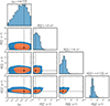 |
Fig. A.1. MCMC inference result for one realization of the mock sample of 14 FRBs in M02 model (see Table A.1). The red (blue) contours correspond to the inferred 68% (95%) confidence intervals. The diagonal panels show the corresponding marginalized 1D posterior probabilities of the model parameters. The black dots with dashed lines illustrate the input true values of the model parameters. |
All Tables
Inference test results for different combinations of the input true model parameters Θ.
All Figures
|
Fig. 1. Left: Distribution of absolute values of RMeg as a function of FRB redshift in observer frame. The black dots show the FRB sample analysed in this work, whereas the grey triangles are the DSA-110 subsample taken from Sherman et al. (2023) and the blue diamonds illustrate the FRBs from the Mannings et al. (2023) sample, which are not part of this work. Right: Distribution of RMeg values in rest-frame of FRB hosts as a function of the corresponding |
| In the text | |
|
Fig. 2. Impact parameter bimpact of identified foreground halos with respect to their virial radius, r200, along each FRB sight line, plotted as a function of the impact parameter. The colour map illustrates the mean mass of the halos, whereas the associated uncertainty is propagated into the error bars on their corresponding r200. The dashed line illustrates the maximum distance, bimpact = r200, at which a foreground halo can be intersected by the FRB sight line and potentially contribute to RMobs if a halo extends to 1 virial radius, r200. In addition, we also show the case where the halos extend to two virial radii, 2 × r200, with the dash-dotted lines. |
| In the text | |
|
Fig. 3. Example of typical distributions of RM values for FRB 20211212A: (left) from the mNFW model of a single foreground galactic halo (see Section 3.3); (middle) from the mNFW model of the corresponding host-galaxy halo (see Section 3.4.1); and (right) from the local environment in the ISM of the host galaxy and/or FRB progenitor (see Section 3.4.2). The positive values of the histograms correspond to the RM values for the case when the line-of-sight component of the magnetic field is aligned with the direction of the FRB sight line (parallel), whereas the negative parts of the histograms, illustrate the case where the line-of-sight component of the magnetic field is directed away from the observer (anti-parallel). The dashed maroon lines show the KDE fit to the resulting RM distributions (see Section 4). Note the different range of RM values in the panels. |
| In the text | |
|
Fig. 4. Resulting distribution of RMmodel values given by Eq. (3), estimated by combining contributions from each environment along the FRB sight line (see Section 3 and Figure 3 for details). The vertical dashed magenta line illustrates the value of the RMobs for FRB 20211212A, while the horizontal magenta dotted line shows the value of the corresponding log-likelihood value (logℒFRB = −6.41) evaluated from the KDE fit to the RMmodel distribution at the value of RMobs, given the combination of model parameters Θ (see discussion in Section 4 for more details). |
| In the text | |
|
Fig. 5. MCMC inference result for sample of 14 FRBs in our dataset (see Table 1). The orange (blue) contours correspond to the inferred 68% (95%) confidence intervals. The diagonal panels show the corresponding marginalised 1D posterior probabilities of the model parameters. |
| In the text | |
|
Fig. 6. 1D marginalised posterior probability distributions of model parameters considered in this work, estimated with different values of ⟨figm⟩ adopted for the fd(z) prior (see Section 4.2). The fiducial model with ⟨figm⟩ = 0.60 is shown by the blue curves. |
| In the text | |
|
Fig. 7. Comparison of B∥ measurements in CGM halos obtained (left panel) and in galactic ISM (right panel), in this (star symbols) and various previous (circles) works. We place |
| In the text | |
|
Fig. A.1. MCMC inference result for one realization of the mock sample of 14 FRBs in M02 model (see Table A.1). The red (blue) contours correspond to the inferred 68% (95%) confidence intervals. The diagonal panels show the corresponding marginalized 1D posterior probabilities of the model parameters. The black dots with dashed lines illustrate the input true values of the model parameters. |
| In the text | |
Current usage metrics show cumulative count of Article Views (full-text article views including HTML views, PDF and ePub downloads, according to the available data) and Abstracts Views on Vision4Press platform.
Data correspond to usage on the plateform after 2015. The current usage metrics is available 48-96 hours after online publication and is updated daily on week days.
Initial download of the metrics may take a while.