| Issue |
A&A
Volume 706, February 2026
|
|
|---|---|---|
| Article Number | A246 | |
| Number of page(s) | 12 | |
| Section | Extragalactic astronomy | |
| DOI | https://doi.org/10.1051/0004-6361/202557228 | |
| Published online | 13 February 2026 | |
H.E.S.S. detection and multi-wavelength study of the z ∼ 1 blazar PKS 0346−27
1
Astronomy & Astrophysics Section, School of Cosmic Physics, Dublin Institute for Advanced Studies, DIAS Dunsink Observatory Dublin D15 XR2R, Ireland
2
Max-Planck-Institut für Kernphysik P.O. Box 103980 D 69029 Heidelberg, Germany
3
University of Namibia, Department of Physics Private Bag 13301 Windhoek 10005, Namibia
4
Centre for Space Research, North-West University Potchefstroom 2520, South Africa
5
Institut für Physik und Astronomie, Universität Potsdam Karl-Liebknecht-Strasse 24/25 D 14476 Potsdam, Germany
6
Université Paris Cité, CNRS, Astroparticule et Cosmologie F-75013 Paris, France
7
Department of Physics and Electrical Engineering, Linnaeus University 351 95 Växjö, Sweden
8
Deutsches Elektronen-Synchrotron DESY Platanenallee 6 15738 Zeuthen, Germany
9
Institut für Physik, Humboldt-Universität zu Berlin Newtonstr. 15 D 12489 Berlin, Germany
10
Institut für Astronomie und Astrophysik, Universität Tübingen Sand 1 D 72076 Tübingen, Germany
11
LUX, Observatoire de Paris, Université PSL, CNRS, Sorbonne Université 5 Pl. Jules Janssen 92190 Meudon, France
12
Sorbonne Université, CNRS/IN2P3, Laboratoire de Physique Nucléaire, et de Hautes Energies, LPNHE 4 place Jussieu 75005 Paris, France
13
IRFU, CEA, Université Paris-Saclay F-91191 Gif-sur-Yvette, France
14
Friedrich-Alexander-Universität Erlangen-Nürnberg, Erlangen Centre for Astroparticle Physics Nikolaus-Fiebiger-Str. 2 91058 Erlangen, Germany
15
School of Physics, University of the Witwatersrand, 1 Jan Smuts Avenue Braamfontein Johannesburg 2050, South Africa
16
School of Physical Sciences and Centre for Astrophysics & Relativity, Dublin City University Glasnevin Dublin D09 W6Y4, Ireland
17
University of Oxford, Department of Physics, Denys Wilkinson Building Keble Road Oxford OX1 3RH, UK
18
Laboratoire Leprince-Ringuet, École Polytechnique, CNRS, Institut Polytechnique de Paris F-91128 Palaiseau, France
19
Aix Marseille Université, CNRS/IN2P3, CPPM Marseille, France
20
Laboratoire Univers et Particules de Montpellier, Université Montpellier, CNRS/IN2P3, CC 72 Place Eugène Bataillon F-34095 Montpellier Cedex 5, France
21
School of Science, Western Sydney University Locked Bag 1797 Penrith South DC NSW 2751, Australia
22
Landessternwarte, Universität Heidelberg Königstuhl D 69117 Heidelberg, Germany
23
Universität Innsbruck, Institut für Astro- und Teilchenphysik Technikerstraße 25 6020 Innsbruck, Austria
24
Universität Hamburg, Institut für Experimentalphysik Luruper Chaussee 149 D 22761 Hamburg, Germany
25
Obserwatorium Astronomiczne, Uniwersytet Jagielloński ul. Orla 171 30-244 Kraków, Poland
26
Institute of Astronomy, Faculty of Physics, Astronomy and Informatics, Nicolaus Copernicus University Grudziadzka 5 87-100 Torun, Poland
27
Nicolaus Copernicus Astronomical Center, Polish Academy of Sciences ul. Bartycka 18 00-716 Warsaw, Poland
28
Instytut Fizyki Jadrowej PAN, ul. Radzikowskiego 152 ul. Radzikowskiego 152 31-342 Kraków, Poland
29
Yerevan Physics Institute 2 Alikhanian Brothers St. 0036 Yerevan, Armenia
30
Kavli Institute for the Physics and Mathematics of the Universe (WPI), The University of Tokyo Institutes for Advanced Study (UTIAS), Japan
31
Department of Physics, Konan University, 8-9-1 Okamoto Higashinada Kobe Hyogo 658-8501, Japan
32
Kapteyn Astronomical Institute, University of Groningen Landleven 12 9747 AD Groningen, The Netherlands
33
GRAPPA, Anton Pannekoek Institute for Astronomy, University of Amsterdam Science Park 904 1098 XH Amsterdam, The Netherlands
★ Corresponding authors: This email address is being protected from spambots. You need JavaScript enabled to view it.
Received:
12
September
2025
Accepted:
20
December
2025
Abstract
Context. PKS 0346-27 is a low synchrotron peaked blazar at redshift 0.991. The very high energy (VHE; E > 100 GeV) spectra of blazars are always affected by γγ absorption by the extragalactic background light (EBL), and subsequently no blazars have been detected in VHE γ-rays at redshifts exceeding 1.
Aims. This is the goal of a target-of-opportunity (ToO) programme by H.E.S.S.: to observe flaring high-redshift (z ≳ 1) blazars. Importantly, extending the redshift range of VHE-detected blazars to z ≳ 1 will yield insights into the cosmological evolution of both the VHE blazar population and the EBL.
Methods. We report H.E.S.S. ToO and multi-wavelength observations of the blazar PKS 0346−27. We analysed and modelled the H.E.S.S. data together with simultaneous data from Fermi-LAT, Swift (XRT and UVOT), using single-zone leptonic and hadronic models.
Results. PKS 0346-27 was detected by H.E.S.S. at a significance of 6.3σ during one night on 3 November 2021, while for other nights before and after this day, upper limits on the VHE flux have been determined. No evidence for intra-night γ-ray variability has been found. A flare in high-energy (E > 100 MeV) γ-rays detected by Fermi-LAT preceded the H.E.S.S. detection by 2 days. A fit with a single-zone emission model to the contemporaneous spectral energy distribution during the detection night was possible with a proton-synchrotron-dominated hadronic model, requiring a proton-kinetic-energy-dominated jet power temporarily exceeding the source’s Eddington limit, although alternative (e.g. multi-zone) models cannot be ruled out. A one-zone leptonic model is, in principle, also able to fit the flare-state spectral energy distribution. However, it requires implausible parameter choices, in particular, extreme Doppler and bulk Lorentz factors of ≳80.
Key words: radiation mechanisms: non-thermal / relativistic processes / galaxies: active / galaxies: individual: PKS 0346–27 / galaxies: jets / quasars: general
Publisher note: The year of the acceptance date was corrected to "2025" in the PDF file on 17 February 2026.
© The Authors 2026
 Open Access article, published by EDP Sciences, under the terms of the Creative Commons Attribution License (https://creativecommons.org/licenses/by/4.0), which permits unrestricted use, distribution, and reproduction in any medium, provided the original work is properly cited.
This article is published in open access under the Subscribe to Open model. This email address is being protected from spambots. You need JavaScript enabled to view it. to support open access publication.
1. Introduction
Blazars are the relativistically boosted class of radio-loud active galactic nuclei (AGN) whose jets are aligned at a small angle to the observer’s line of sight (Urry & Padovani 1995). Based on their optical spectra, they are classified into two sub-classes: flat-spectrum radio quasars (FSRQs) which have broad emission lines, and BL Lacertae objects (BL Lacs) which have weak or no emission lines (Stocke et al. 1991; Sambruna et al. 1996). The broadband spectral energy distributions (SEDs) of blazars show a typical double-peaked structure peaking in the infrared (IR) to X-ray for the low-energy component and in the megaelectronvolt to teraelectronvolt bands for the high-energy component. The low-energy component is well explained by synchrotron emission from relativistic electrons in the jet, while the emission processes giving rise to the high-energy emission peak are not fully understood yet, as several emission mechanisms could be responsible. In the leptonic model, the high-energy gamma-ray radiation results from the inverse-Compton scattering of soft target photons originating in the synchrotron radiation process (Sikora et al. 2009) or external photon fields (e.g. Dermer et al. 1992). Alternatively, in hadronic models (Mücke & Protheroe 2001; Böttcher et al. 2013), part of the high-energy emission originates from proton synchrotron radiation or the decay products following photo-pion interactions of relativistic protons.
Based on the location of their synchrotron peak frequency (νpeak, sync), blazars are also classified into three categories: low-synchrotron-peaked (LSP) blazars, which have νpeak, sync < 1014 Hz, intermediate-synchrotron-peaked (ISP) blazars, which have 1014 Hz ≤νpeak, sync ≤ 1015 Hz and high-synchrotron-peaked (HSP) blazars with νpeak, sync > 1015 Hz (Abdo et al. 2010a). Occasionally, low-synchrotron-peaked sources transition to an ISP character during their flaring state (Foschini et al. 2008; Cutini et al. 2014; Ahnen et al. 2015).
The γγ pair production through the interaction of γ-ray photons with low-energy photons (infrared and optical) from diffuse extragalactic background light (EBL) limits the possibility of detecting blazars above 100 GeV from sources at cosmological distances (Salamon & Stecker 1998). This absorption effect increases with distance and energy of the very high energy (VHE) photons. Therefore VHE blazars (usually not detected beyond redshift ∼0.5) at redshift ∼1 are expected to be severely affected by EBL absorption. However, this absorption can be used to constrain this EBL effect, especially for high redshift sources. With this science objective, the High Energy Stereoscopic System (H.E.S.S.) collaboration has a target-of-opportunity (ToO) programme in place to trigger H.E.S.S. and coordinated multi-wavelength observations of high redshift (z ≳ 1) blazars in flaring states identified by the Fermi Large Area Telescope (H.E.S.S. Collaboration 2024).
The FSRQ PKS 0346-27 was first identified as a radio source in the Parkes catalogue (Bolton et al. 1964) and later classified as a quasar by White et al. (1988) based on its optical spectrum. It was detected as an X-ray source by ROSAT (Voges et al. 1999) and as a γ-ray source by Fermi-LAT and included in the Fermi-LAT First Source catalogue (1FGL; Abdo et al. 2010b). In the Fermi -LAT fourth source catalogue (4FGL; Abdollahi et al. 2020) it is associated with the γ-ray source 4FGL J0348.5-2749. On 2 February 2018 (MJD 58151), Angioni (2018) reported a strong γ-ray flare based on Fermi-LAT data. This prompted multi-wavelength follow-up observations in the optical – near-infrared (NIR) (Nesci 2018a; Vallely et al. 2018), ultraviolet (UV), and X-ray (Nesci 2018b), which also showed enhanced activity of this source. Kamaram et al. (2023) studied the long-term variability of PKS 0346-27 from December 2019 to January 2021 (MJD 58484-59575) with multi-wavelength data from Fermi-LAT, Swift-X-Ray Telescope (XRT), and UV-optical Telescope (UVOT) and found five flaring episodes during this period of study with a minimum variability timescale of ∼1 day and ∼0.1 days for the γ-ray and X-ray light curves, respectively.
In this paper, we report on the first VHE γ-ray detection of this source by H.E.S.S. on 3 November 2021 (MJD 59521.97) from observations triggered by a γ-ray flare detected by Fermi-LAT. Contemporaneous multi-wavelength data from H.E.S.S, Fermi-LAT, Automatic Telescope for Optical Monitoring (ATOM), Swift-XRT, and UVOT during this flare are presented. We modelled the SED of this source using the leptonic and hadronic code by Böttcher et al. (2013) and constrained the effects of the EBL using the EBL model by Finke et al. (2010). In Section 2, we discuss the multi-wavelength observations and analysis techniques for the different telescopes and present the multi-wavelength SED and light curves. The SED modelling of the source is discussed in Section 3. We present a summary and our conclusions in Section 4.
2. Observation and data analysis
2.1. H.E.S.S. observations and analysis techniques
The H.E.S.S. array consists of five telescopes located in the Southern Hemisphere in Namibia at an altitude of 1800 m. It detects VHE γ-rays using the atmospheric Cherenkov imaging technique (Holler et al. 2015). In 2003, the first phase consisting of four 12m diameter telescopes (CT1-4), arranged on a 120m side square, started operations. It was sensitive to γ-rays above a few hundred gigaelectrovolt energies. In 2012, an additional 28m telescope (CT5) was added in the middle of the four 12m telescopes, which lowered the detection threshold of the array.
H.E.S.S. observation data were collected in observation runs of approximately 28 mins. The data taken with the four 12m telescopes (CT1-4) are referred to as ‘stereo’ data, while the data collected with only CT5 are called ‘mono’ data. Each of the five telescopes images the Cherenkov light emitted by particle showers triggered by the interaction of γ-rays or cosmic rays with the Earth’s atmosphere. A probabilistic distinction between cosmic-ray and γ-ray induced showers is done based on the characteristics of the shower images. The study of the shower images allows for reconstruction of the primary particle’s direction, energy, and arrival time.
The ToO observations of PKS 0346-27 with H.E.S.S. were triggered on 30 October 2021 (MJD 59517.97) by FlaapLUC (Lenain 2018) following the detection of flaring activity by Fermi-LAT. H.E.S.S. observations were carried out with all five telescopes during the observation period (30 October to 8 November 2021, MJD 59517.97 to 59525.94). The observations were done in wobble mode, where the telescopes point at 0.5° from the source position to allow simultaneous background estimation (Berge et al. 2007). Data quality cuts were applied to remove periods affected by poor weather conditions and hardware problems. After applying the quality criteria, 34 runs were selected for the entire observation period, out of which four runs were selected for the detection night (MJD 59521.97).
For only the CT1-4 dataset, the H.E.S.S. data for all the observation periods were analysed with the Image Pixel-wise fit for Atmospheric Cherenkov Telescope (IMPACT) analysis chain (Parsons & Hinton 2014). The analysis was cross-checked with another analysis chain (de Naurois & Rolland 2009), and this yielded a consistent result. Another independent analysis was performed with only the CT5 dataset using the neural network-based chain described in Murach et al. (2015).
The analysis of the CT1-4 dataset yielded an excess of 50.8 γ-like events and a signal-to-background ratio of 0.03 for 16.6 h livetime. Using Eq. (17) of Li & Ma (1983) a significance of 1.3σ was obtained for the entire dataset after background subtraction using the ring background method (H.E.S.S. Collaboration 2006), which resulted in 1618 ON and 35372 OFF events, while the average number of OFF regions (α) is 9.24. The signal-to-background ratio is defined as excess over background, where background (B) = (# OFF events)/α. The analysis of the CT5 dataset yielded an excess of 208.1 γ-like events corresponding to 3.6σ for 16.8 h livetime. When analysing individual nights, only one night (3 November 2021) showed a significant greater-than-5σ detection. Therefore, upper limits were generated for both spectral and light curve analyses for all other observation nights at a 99 % confidence level following Rolke et al. (2005).
Figure 1 shows the sky maps and the on-source and normalised off-region distributions as a function of squared angular distance from the source (i.e. θ2 plots) for the detection night for both analysis chains. The four runs passed the quality selection criteria. The analysis yielded an excess of 78.0 γ-like events and a signal-to-background ratio of 0.4 for 1.8 h livetime, resulting in a significance of 5.4σ for CT1-4, while for CT5, it generated an excess of 132.5 γ-like events for 1.9 h livetime and a significance of 6.3σ. The ring background method was used for background subtraction, which resulted in 251 ON and 3968 OFF events for CT1-4 and 488 ON and 4219 OFF events for CT5. The energy threshold for CT1-4 is 133 GeV, and it is 121 GeV for CT5. Only the detection night analysis was used for the spectral modelling, while all observation nights were used to generate the H.E.S.S. light curve, using the photon index from the detection night. The reflected background method (H.E.S.S. Collaboration 2006) was used for the spectral analysis for both analysis chains. The spectrum was fitted with a power-law function:
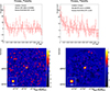 |
Fig. 1. Result for θ2 from the 3 November 2021 (MJD 59521.93 – 59521.99) observation night analysis and significance plots with the four selected runs. Top-left and bottom-left panels: Results from the CT1-4 dataset. Top-right and bottom-right panels: Results from the CT5 dataset. The inset shows the point spread function, which was derived by fitting the θ2 distribution to the KING’s function, described in Ackermann et al. (2013). |
 (1)
(1)
where N0 is the differential photon flux normalisation at the reference energy, E0, and Γ is the photon index.
The systematic errors were derived separately following H.E.S.S. Collaboration (2022). Multiple sources of systematic errors were taken into account. For the CT1-4 analysis, the systematic uncertainties derived from the different analysis cuts are 5% on the flux normalisation and 0.1 on the index. The atmospheric transparency contributes a relative uncertainty of 10% on the flux normalisation and 0.05 on the index. For the CT5 analysis, the systematic error due to the imperfect background acceptance description is 15% on the flux normalisation and 0.15 on the index, while the atmospheric transparency contributes 7% on the flux normalisation and 0.15 on the index, respectively. The systematic uncertainty on the flux normalisation derived from the uncertainty of the absolute energy scale, which is assumed to be 10%, is estimated as (1 ± 10%)Γ. All of these contributions were added in quadrature to obtain the overall systematic errors listed in Tab. 1 with spectral parameters.
Very high energy γ-ray spectral parameters for the detection night of 3 November 2021.
Figure 2 shows the energy spectrum where each flux point was re-binned to achieve a minimum significance of 2σ per bin (forward-folding method). The butterfly-shaped areas indicate the statistical errors (orange) and systematic together with statistical errors (purple). Figure 2 shows both the observed and EBL-corrected flux points using the model of Finke et al. (2010).
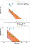 |
Fig. 2. Observed spectra and flux points together with intrinsic flux points for the CT1-4 (top panel) and CT5 (bottom panel) dataset. The observed spectrum and flux points were de-absorbed with the Finke et al. (2010) EBL model. The orange bands are the statistical errors only, while the purple bands show the systematic errors together with the statistical errors. The error bars of the flux points are statistical only. |
2.2. Fermi-LAT data analysis
The LAT is the primary instrument onboard the Fermi satellite (Atwood et al. 2009) sensitive to γ-rays with energies from ∼20 MeV to beyond 300 GeV. It enables high sensitivity measurements and operates in full-sky survey mode, covering the entire sky approximately every 3 hours.
Fermi-LAT data taken between 28 October and 8 November 2021 (MJD 59515.5 – 59526.5) were retrieved from the Fermi Science Support Center data server1 and analysed using Fermitools version 2.2.0 along with P8R3_SOURCE_V3 instrument response functions. Only source class events (event class 128 and event type 3) were selected in the 15° region of interest (ROI), centred around the position of the point source 4FGL J0348.6−2749 associated with PKS 0346−27, with energies between 100 MeV and 300 GeV. A maximum zenith angle cut of 90° was applied to filter out the Earth’s limb contamination. The gll_iem_v07 and iso_P8R3_SOURCE_V3_v1 models were used to account for the diffuse Galactic and extra-galactic isotropic background emissions, respectively.
A binned likelihood analysis was performed in an iterative manner. The initial input source model was composed of the entire 12-year Fermi-LAT catalogue (4FGL-DR3) of sources (Abdollahi et al. 2020) that lie in the 15° ROI centred around the position of 4FGL J0348.6−2749, with an additional 10° area added by the make4FGLxml.py tool to avoid event leakage. The parameters of all sources contributing less than 5% of the total measured counts and with a test statistic (TS) below 9, were kept constant. Finally, only parameters of sources located within a 3° separation from the target of interest and that were not frozen in the previous steps were allowed to vary along with the normalisation factors of the two diffuse background models.
Fermi-LAT light curves for the 28 October to 8 November 2021 period centred around the VHE detection night, with daily and 12 h time bins, were derived. They exhibit strong flux variability, with fractional variability amplitude (Vaughan et al. 2003) Fvar = (82 ± 5)%. A maximum daily binned flux value (> 100 MeV) of (3.14 ± 0.25) 10−6 ph cm−2 s−1 was measured. A comparable (historical) maximum was only announced in April 2019 (ATel#12693, Gokus & Angioni 2019). The authors also reported a significant spectral hardening with respect to the first release of the 4FGL (8 year Fermi-LAT catalogue), where the average powerlaw (PL) index of the source was 2.43 ± 0.05. Indeed, PKS 0346−27 remained in a persistent very low state until the end of 2017 to early 2018, when it started flaring for more than 3 years (according to the Fermi-LAT Light Curve Repository2). This changing behaviour is reflected in the spectral index and variability amplitude values that were published later, with more recent releases of the 4FGL catalogue (e.g. 12-year LAT catalogue 4FGL-DR3 covering its brightest γ-ray states) where the spectral index hardened to 2.08 ± 0.01 and the variability index of the source increased by a factor of 180. The spectral indices obtained during the considered campaign showed no significant variability, with a mean value of 1.98 ± 0.22, which appears harder than the aforementioned older catalogue values, but is compatible within errors with the more recent 12 year catalogue value of 2.08 ± 0.01.
The highest energy photon (E ≳ 14 GeV, with at least a 95% chance of being associated with the source of interest) was detected at 03:47:30 UTC on 2 November 2021 (∼MJD 59520.16) at the peak of the Fermi-LAT light curve, that is, approximately two days before the H.E.S.S. detection. No VHE observations were available on the day of the Fermi-LAT light-curve peak. The one-day long time window centred around the H.E.S.S. detection night was analysed separately and yielded a 7.2σ detection (TS = 52) when using a PL model. Although the source is characterised by a significant spectral curvature in the 4FGL-DR3 catalogue (ΔTS = 347), no curvature was found for the one day-long period centred around the H.E.S.S. detection night. A PL index of 1.99 ± 0.21 was derived, and it is compatible with the 4FGL-DR3 catalogue value of 2.08 ± 0.01, while using a LogPar spectral model yields a TS of 46, a log-parabolic index of α = 1.84 ± 0.32, and a curvature parameter (β = 0.19 ± 0.22) compatible with zero.
2.3. Swift data analysis
Simultaneous to H.E.S.S. and Fermi-LAT, PKS 0346-27 was also observed by the Neil Gehrels observatory with both the Swift-XRT and the Swift-UVOT. The XRT is sensitive within the energy range of 0.2–10.0 keV, while the UVOT observes at UV-optical wavelengths of 170–650 nm with V, B, and U filters in the optical and W1, M2, and W2 in the UV. During the observation period (MJD 59517 to 59526), PKS 0346-27 was observed by Swift on three nights, namely MJD 59521.79 (the H.E.S.S. detection night), MJD 59523.78, and 59525.91 (observation IDs 00038373036, 00038373037, 00038373040, respectively) for a total exposure period of 5.9 ks. Only the detection night was considered for the SED modelling, while all three observation periods were used to construct light curves.
2.3.1. Swift-XRT
The XRT data were analysed with available tools on Heasoft software. To reduce the data, we used the standard XRT-PIPELINE to produce clean event files, using the calibration version CALDB 20220331. The cleaned event files corresponding to the photon counting (PC) mode were used to produce the source and background spectra using the XSELECT tool. For the source and background extractions, we considered circular regions of 20 arcseconds and 40 arcseconds, respectively.
The ancillary response file (ARF) and redistribution matrix file (RMF), were generated with xrtmkarf and quizcif, respectively. The source spectrum, background spectrum, RMF and ARF files were then merged using the grppha tool, with each bin accommodating ten counts for Xspec analysis. The spectrum for each observation was fit with an absorbed power-law model and column density, NH = 8.16 × 1019 cm−2 (Bekhti et al. 2016), resulting in photon indices of 1.74 ± 0.23, 1.87 ± 0.29, and 2.2 ± 0.28, respectively.
2.3.2. Swift-UVOT
PKS 0346-27 was also observed by Swift-UVOT in the same observation periods as Swift-XRT for a total observation duration of 5.8 ks. For the spectral and light curve analysis, the uvotsource tool was used to extract the magnitudes from the images taken with each filter (V, B, U, UVW1, UVM2, UVW2) considering source and background regions with radii of 5 arcsecs and 10 arcsecs, respectively. The observed magnitudes were corrected for Galactic extinction with E(B − V) = 0.0094 mag (Schlafly & Finkbeiner 2011) and the extinction ratios for each filter from Giommi et al. (2006). The magnitudes were converted to flux points with the photometric zero points from Breeveld et al. (2011) and the conversion factors provided by Giommi et al. (2006).
2.3.3. ATOM
The Automatic Telescope for Optical Monitoring is a 75 cm telescope located at the H.E.S.S. site in Namibia (Hauser et al. 2004). ATOM monitored PKS 0346-27 on a daily cadence in Bessel B and R filters, with denser coverage and additional V band observations during several nights. The ATOM data were analysed using the fully automated ATOM Data Reduction and Analysis Software, and their quality has been checked manually. Absolute flux was obtained via differential photometry using up to six custom calibrated comparison stars in the same field of view. The results were extinction-corrected following Schlafly & Finkbeiner (2011).
3. Results and discussion
3.1. Multi-wavelength light curves
The multi-wavelength light curve for the entire observation period from 30 October (MJD 59517.97) to 8 November 2021 (MJD 59525.94) for all the telescopes is shown in Fig. 3. On the H.E.S.S. detection night (MJD 59521.97), Swift observed the source 5 hours before, while ATOM observed an hour after H.E.S.S. The VHE γ-ray night-wise light curves using CT1-4 and CT5 data are shown in the first and second panels, while the high-energy γ-ray light curves displayed in the third panel were obtained for daily and 12 hr binnings, respectively. As seen in the Fermi-LAT light curve, the source exhibits a strong flux variability and a peak flux of (3.1 ± 0.25)×10−6 ph cm−2 s−1 on 1 November, 2021 (MJD 59519.9). There was no significant flaring activity seen in both Swift XRT and UVOT during the H.E.S.S. flaring period, although there was a flux increase in the UVOT bands. For example, in the U-band, from the first observation night (MJD 59521.79) with a flux of (2.3 ± 0.10)×10−12 erg cm−2 s−1, it increased to (3.0 ± 0.14)×10−12 erg cm−2 s−1 on 5 November (MJD 59523.78), i.e. 2 days after the H.E.S.S. flare detection. This increased flux can also be observed in other filters. There is also an obvious flux increase in the ATOM R filter on 4 November, 2021 (MJD 59522.03), with flux of (3.6 ± 0.13)×10−12 erg cm−2 s−1, almost during the time of the H.E.S.S. flare. This flaring activity in ATOM continued until 5th November, 2021 (MJD 59523.85) with a peak flux of (4.2 ± 0.10)×10−12 erg cm−2 s−1, and it gradually reduced until the last observation night.
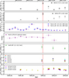 |
Fig. 3. Multi-wavelength light curves from MJD 59515.99 – 59526.10. Panels from top to bottom: H.E.S.S flux for CT1-4 and CT5 in 10−11 cm−2 s−1, Fermi-LAT flux for both 12-h and 24-h binning in 10−6 cm−2 s−1, Fermi-LAT spectral index for 24-h binning, Swift-XRT flux in 10−12 erg cm−2 s−1, Swift-UVOT flux in 10−12 erg cm−2 s−1, and ATOM flux for V, B and R filters in 10−12 erg cm−2 s−1. The double vertical dotted red lines denote the H.E.S.S. detection period, MJD 59521.93 – 59521.99. Only statistical errors are shown. |
Most notably, the VHE flare appears to be delayed by about 2 days with respect to the GeV flare; the GeV flare had already subsided during the H.E.S.S. flaring period. However, there was no observation in the VHE band during the high energy flaring period, so a simultaneous high energy-VHE flare during that night cannot be excluded. Delayed flares between the high-energy and VHE energy bands have previously been observed in 3C 279 (Emery et al. 2019) and between VHE and X-ray bands in 1ES 1959+650 (Krawczynski et al. 2004). The mechanism that causes delayed flares is unknown and a matter of debate. Two possibilities are briefly discussed in Section 3.3.
3.2. Broadband SED modelling
We compiled an SED of PKS 0346-27 using observations by H.E.S.S., Fermi-LAT, ATOM, and Swift-XRT and -UVOT, considering only the detection night. Figure 4 shows the broadband SED of PKS 0346-27 modelled using a single-zone, time-independent hadronic code by Böttcher et al. (2013). This model assumes a spherical emitting region of co-moving radius R filled with a tangled magnetic field B and propagating with a bulk Lorentz factor Γ along the jet at an angle θ with respect to the observer’s line of sight, resulting in relativistic Doppler boosting by a Doppler factor of δ = (Γ [1−βΓ cos θ])−1, where βΓ is the normalised velocity corresponding to the Lorentz factor, Γ. Primary populations of relativistic, non-thermal electrons and protons were injected into the emitting region with a power-law distribution,  , where H is the Heaviside function defined as H = 1 if a ≤ x ≤ b and H = 0 otherwise. The code reaches an equilibrium between the relativistic particle injection, radiative cooling due to various radiative processes (e.g. synchrotron radiation, photo-pion production), and escape on a timescale of tesc = ηesc R/c, where ηesc ≥1 is a free escape timescale parameter. The synchrotron emission from the injected electrons forms the predominant target photon field for proton-photon interactions.
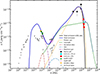 |
Fig. 4. Spectral energy distribution of PKS 0346-27 during the H.E.S.S. detection night of 3 November 2021 fit with a hadronic single-zone model. The individual radiation components are shown without EBL absorption, and they add up to the total intrinsic model SED shown by the solid blue curve. The solid black line shows the total model curve accounting for EBL absorption following the Finke et al. (2010) model. The Fermi-LAT emission is explained by the proton-synchrotron component while the casacade component explains the H.E.S.S. emission. The archival flux points are from https://tools.ssdc.asi.it/SED/. We refer to Table 2 for model parameters. |
The low-energy component of the SED fit was generated by electrons through synchrotron radiation, while proton-synchrotron emission and the synchrotron emission from secondaries produced in proton-photon (photo-pion) interactions account for the high energy component of the SED. Protons interact with the target photon field produced by the primary electrons and generate mesons (π0, π− and π+). π0 decay into photons, while charged pions decay into muons and neutrinos; the muons further decay into electrons/positrons and further neutrinos.
Figure 4 shows the model SED with the EBL absorption taken into account following Finke et al. (2010). Other EBL models were also used, but they resulted in virtually indistinguishable VHE spectra. The Fermi-LAT spectrum is dominated by proton-synchrotron emission, while the H.E.S.S. spectrum is dominated by photo-pion induced cascade emission.
Table 2 lists all relevant parameters used to produce the SED fit. However, we note that there are substantial parameter degeneracies, so the listed parameter values only represent one possible realisation of a hadronic single-zone fit and should not be taken as a unique solution. Except for the redshift and the black hole mass (see below), none of the parameters can be reliably constrained from independent observations. Therefore, they were left free, with the aim of minimising the required jet power and being in line with previous hadronic modelling results of FSRQs (e.g. Böttcher et al. 2013).
In our hadronic SED fit, the jet power is dominated by the kinetic energy of the relativistic protons, leading to energy partition fractions of LB/Le = 7.4 × 10³ and LB/Lp = 0.6. The mass of the supermassive black hole in PKS 0346-27, MBH ∼ 2 × 10⁸ M⊙, as estimated by Angioni et al. (2019), corresponds to an Eddington luminosity of LEdd ∼ 2.5 × 1046 erg s−1. Notably, the total jet power required by our model fit therefore exceeds the Eddington luminosity by a factor of approximately six during the H.E.S.S. detection night. However, as the modelled SED represents a short-term flare state, the Eddington limit needs to be surpassed only for the ≲1 day duration of the flare and not persistently.
The steep optical (electron-synchrotron) spectrum necessitates a steep electron injection index of q = 3.5, which is significantly steeper than expected from, for example, non-relativistic shock acceleration (q = 2). However, if shock acceleration is the dominant non-thermal particle-energisation mechanism, the shocks in AGN jets are likely to be at least mildly relativistic and oblique. In such a case, spectral indices significantly exceeding two may result from diffusive shock acceleration (e.g. Summerlin & Baring 2012).
We also attempted a fit with a single-zone leptonic model. However, as we show below and in the Appendix, such a scenario would require extreme and implausible parameter choices. To illustrate the general problem with a single-zone leptonic interpretation, we started with the standard assumption that inverse Compton scattering of an external target photon field is responsible for the γ-ray emission. In order to achieve external Compton (EC) emission in the Thomson regime extending into the VHE range, a low-energy target photon field is required, plausibly provided by the dusty torus of temperature TDT ≡ 103 T3 K, with T3 ∼ 1 – a few being a parameter. The νFν peak frequency of EC scattering of dusty torus photons (EC[DT]) by a relativistic electron population with a break or low-energy cut-off at γb is given by  if Compton scattering occurs in the Thomson regime, which we will verify a posteriori. Given the required steep electron spectrum, this peak frequency must be located above the Fermi-LAT energy range, in order to avoid overproduce the gigaelectronvolt γ-ray flux. Assuming the EC(DT) peak frequency to be at a dimensionless energy,
  , we required a break electron energy of γb ∼ 6 × 10⁴ (Γ1 δ1 T3)−1/2, where we use the standard nomenclature of Qi =Q/(10i[c.g.s]). As the target photon energy in the co-moving frame is ϵ′t ∼ 5 × 10⁻⁶ Γ1 T3, we found that ϵ′tγb ∼ 0.3 T31/2 (Γ1/δ1)1/2, which confirms our assumption that Compton scattering occurs in the Thomson regime at the peak of the γ-ray spectrum as long as δ ≈ Γ. The steep optical – UV spectrum indicates that the synchrotron peak is located at
  Hz, leading to a magnetic-field estimate of B ≲ 6 Γ1 T3 mG, much lower than the approximately Gauss magnetic fields typically found in SED modelling of FSRQs (e.g. Aleksić et al. 2011; Zacharias et al. 2017; Angioni et al. 2019). The Poynting-flux power carried by the jet of cross-sectional radius RB ≡ 1016 R16 cm, is LB ≲ 1.4 × 1039 Γ14 T32 R162 erg s−1. As the power in relativistic electrons in the jet has to be at least as large as the radiated power (dominated by the γ-ray emission with (νFν)EC ∼ 10−10 erg cm−2 s−1), we have a lower limit on Le ≳ 4π dL2 (νFν)EC/Γ2 ∼ 5 × 1046 Γ1−2 erg s−1, where we used a luminosity distance of dL ∼ 2 × 1028 cm. Thus, the jet would need to be extremely far out of equipartition, dominated by electron kinetic energy by a factor of LB/Le ≲ 3 × 10⁻⁸ Γ16 R162 T32, while the ≲ day-scale variability observed (tvar ≡ 1 td day) constrains the size of the emission region to R16 ≲ 1.3 td δ1. Thus, for any plausible choice of parameters, the jet would be unreasonably strongly dominated by kinetic energy.
Another problem becomes obvious when evaluating the co-moving synchrotron photon energy density,  erg cm−3. When comparing this to the magnetic field energy density, u′B ≲ 10−7 Γ12 T32 erg cm−3, we found that a ratio of synchrotron self-Compton (SSC) to synchrotron peak fluxes of
  would result. Given that this SSC dominance should not exceed the observed Compton dominance of about ten, we can infer Γ ∼ δ ≳ 80 (R16 T3)−1/3, which is unusually large compared to the typically inferred Doppler and bulk Lorentz factors of ∼10–50 (Lister 2016), although Homan et al. (2021) reported Doppler factors greater than 100 for several blazars studied in the radio band. The above estimates illustrate that a single-zone leptonic model has great difficulty producing the observed flare-state SED with plausible parameter values.
An example of a fit attempt using parameters similar to those constrained above is presented in the Appendix. It illustrates that a single-zone leptonic model with Γ = δ = 80 is able to reproduce the flare-state SED of PKS 0346-27. However, the fit requires extreme parameters: exceedingly large Doppler and bulk Lorentz factors, an unusually small magnetic field of 48 mG (compared to SED fit results for other FSRQ-type blazars), and particle energy dominating over magnetic field energy by over five orders of magnitude. We therefore disfavour such a scenario. Thus, when restricting the model consideration to a basic one-zone model, the hadronic model discussed above was considered the most plausible interpretation. Leptonic multi-zone models with two or more zones contributing jointly to produce a broad high-energy emission component can, of course, not be ruled out, but their consideration is beyond the scope of this paper. As the hadronic single-zone model is the model with the fewest additional parameters beyond a single-zone leptonic model and it provides a plausible SED fit, we consider it preferred.
Difficulties with SED fitting using a single-zone leptonic model have also been found in other IACT-detected FSRQs. For example, the steep optical – UV spectrum of 3C279, compared to the hard and broad γ-ray SED, extending into the VHE regime, made such a single-zone leptonic fit implausible, leading to a strong preference for a hadronic interpretation (Boettcher et al. 2009). In the case of PKS 1510-089 (H.E.S.S. Collaboration 2023), the uncorrelated variability in 2021-22, with the X-ray and VHE emissions remaining at almost unchanged levels, while the optical and Fermi-LAT γ-ray emissions dropped abruptly in 2021, provided a strong preference for two-zone interpretation.
We note, however, that the SEDs of other VHE-detected FSRQs could be plausibly reproduced with single-zone leptonic models: The SEDs of PKS 1441+25 (Ahnen et al. 2015; Abeysekara et al. 2015), PKS 1222+216, and TON 599 (Adams et al. 2022) could all be modelled with single-zone leptonic scenarios. Even the SED of PKS 1510-089 during an outburst in 2015 could be well represented with such a model, although with less unusual variability features than the 2021-2022 period mentioned above (Ahnen et al. 2017). In most of these cases, there is evidence of synchrotron emission making a significant contribution to the X-ray emission as well as significantly harder Fermi-LAT (and in most cases also harder IR – optical – UV synchrotron) spectra than found in PKS 0346-27, which indicates harder electron spectra, extending to higher electron energies, facilitating a leptonic high-energy emission interpretation.
3.3. Possible causes of TeV – GeV flare delays
The possible delay of the VHE flare on MJD 59521.9, ∼2 days after the peak of the Fermi-LAT flare deserves special consideration. While no contemporaneous H.E.S.S. observations were possible during the high-energy flare (and therefore we cannot exclude a simultaneous high-energy plus VHE γ-ray flare) the VHE flare during the H.E.S.S. detection night clearly appears as a VHE flare without a simultaneous counterpart in high-energy γ-rays. Various models have been suggested for delayed γ-ray flares, including the class of synchrotron mirror models in which synchrotron radiation from the dominant jet emission region is reflected off stationary (or non-relativistically moving) clouds or sheaths near the jet trajectory and re-enters the jet to act as an enhanced target photon field for Compton scattering in leptonic emission scenarios (Ghisellini & Madau 1996; Böttcher & Dermer 1998; Bednarek 1998; Vittorini et al. 2014; Tavani et al. 2015; MacDonald et al. 2015, 2017; Böttcher 2021) or for photo-pion production in hadronic scenarios (Böttcher 2005; Oberholzer & Böttcher 2018). The latter model may lead to an orphan VHE flare due to enhanced γ-ray production from pion decay and subsequent electromagnetic cascades, while the high-energy γ-ray emission is dominated by proton-synchrotron emission (as in the case of our SED fit presented above), which is not significantly affected by the enhanced external radiation field. Such a scenario would require the reflecting material to be located at a distance of Rm ∼ 2Γ2 cΔt/(1 + z), where Δt ∼ 2 days is the delay between the primary high-energy γ-ray flare and delayed VHE flare. With the value of Γ = 10 adopted for our hadronic SED fit, this would yield a distance of Rm ∼ 0.2 pc, a plausible location of an isolated broad-line region cloud. Detailed modelling of this flare with such a hadronic synchrotron mirror model is beyond the scope of this paper and is therefore left to future work.
An alternative explanation could be a finite acceleration time of protons producing the VHE γ-ray emission via proton synchrotron radiation (see, e.g. H.E.S.S. Collaboration 2022, for an application of a similar scenario to the delayed VHE emission from the recurrent nova RS Ophiuchi). The proton acceleration timescale for a generic acceleration process for the highest-energy protons of energy γp, max = 5 × 10⁹ (B/45G)−1/2 δ1−1/2 may be parameterised as
 (2)
(2)
with an acceleration efficiency parameter ηa ≥ 1, where the prime indicates the time in the co-moving frame of the emission region. For this acceleration time to equal the co-moving-frame time delay between the Fermi-LAT and H.E.S.S. flares, Δt′=Δtobs δ/(1 + z)≈9 × 10⁵ δ1 s, we required an acceleration efficiency factor of
 (3)
(3)
a plausible value for a moderately efficient acceleration process. The synchrotron cooling timescale for protons of energy γp, max is
 (4)
(4)
which is of the same order of magnitude as the acceleration timescale from Eq. 2 (with ηa = 75), so the radiative cooling shuts off the acceleration when protons reach the energy γp, max. The Larmor radius of protons of such energy is rL ≈ 3.5 × 10¹⁴ (B/45 G)−3/2 δ1−1/2 cm and thus smaller than the size of the emission region used for our SED modelling. Hence, the protons required for producing the VHE γ-ray proton-synchrotron emission can be confined well within the emission region by a magnetic field of ∼45 G.
This scenario, however, faces two problems. First, it does not explain why the Fermi-LAT flux has decreased back to quiescent levels at the time of the H.E.S.S. flare, as the acceleration process is still active, and the synchrotron cooling timescale for protons producing the high-energy γ-ray emission is longer than 2 days in the observer’s frame. Second, even the cooling timescale for protons producing the VHE emission is ≈2 days, so that additional factors – possibly a swing of the motion of the emission region away from the line of sight (e.g. Britzen et al. 2017, 2023) or a decreasing magnetic field on a time scale of ∼1 day in the observer’s frame (see, e.g., Thiersen et al. 2022, 2024, for a study of magnetic-field changes on the long-term variability of blazars) – must be invoked in order to explain the VHE flare duration of less than 1 day.
4. Summary and conclusions
In this paper, we have reported on the VHE γ-ray detection of the low-synchrotron-peaked blazar PKS 0346-27 by H.E.S.S. on 3 November 2021 as well as contemporaneous multi-wavelength observations. At the time of the announcement of its detection (Wagner et al. 2021), PKS 0346-27 was the most distant VHE-detected blazar at z = 0.991 (this has now been superseded by OP 313 at z = 0.997, detected by the CTAO LST-1, Cortina & CTAO LST Collaboration 2023). Day-scale γ-ray variability was found. H.E.S.S. detected the source in only one night, ∼2 days after the peak of a prominent high-energy γ-ray flare detected by Fermi-LAT, which had subsided at the time of the H.E.S.S. detection. The broadband SED on the day of the H.E.S.S. detection could be satisfactorily modelled with a proton-synchrotron dominated single-zone hadronic model with temporarily super-Eddington jet power. In the framework of such a hadronic model, the potentially delayed VHE flare could possibly be explained with a hadronic synchrotron mirror model or a scenario of gradual proton acceleration, although the latter scenario faces significant challenges. Detailed model simulations of such scenarios are left to future work. Alternatively, a fit with a single-zone leptonic model is, in principle, also possible, but it requires extreme Doppler and bulk Lorentz factors of ∼80, an unusually low magnetic field (compared to SED fitting results of other FSRQs), and an energy ratio between relativistic electrons and magnetic fields far out of equipartition by more than five orders of magnitude. We therefore favour the hadronic model interpretation. Multi-zone models are another alternative that might provide a satisfactory SED fit, but their exploration is beyond the scope of this paper.
Acknowledgments
The support of the Namibian authorities and of the University of Namibia in facilitating the construction and operation of H.E.S.S. is gratefully acknowledged, as is the support by the German Ministry for Education and Research (BMBF), the Max Planck Society, the German Research Foundation (DFG), the Helmholtz Association, the Alexander von Humboldt Foundation, the French Ministry of Higher Education, Research and Innovation, the Centre National de la Recherche Scientifique (CNRS/IN2P3 and CNRS/INSU), the Commissariat à l’Énergie atomique et aux Énergies alternatives (CEA), the U.K. Science and Technology Facilities Council (STFC), the Irish Research Council (IRC) and the Science Foundation Ireland (SFI), the Knut and Alice Wallenberg Foundation, the Polish Ministry of Education and Science, agreement no. 2021/WK/06, the South African Department of Science and Technology and National Research Foundation, the University of Namibia, the National Commission on Research, Science and Technology of Namibia (NCRST), the Austrian Federal Ministry of Education, Science and Research and the Austrian Science Fund (FWF), the Australian Research Council (ARC), the Japan Society for the Promotion of Science, the University of Amsterdam and the Science Committee of Armenia grant 21AG-1C085. We appreciate the excellent work of the technical support staff in Berlin, Zeuthen, Heidelberg, Palaiseau, Paris, Saclay, Tübingen and in Namibia in the construction and operation of the equipment. This work benefited from services provided by the H.E.S.S. Virtual Organisation, supported by the national resource providers of the EGI Federation.
References
- Abdo, A. A., Ackermann, M., Agudo, I., et al. 2010a, ApJ, 716, 30 [NASA ADS] [CrossRef] [Google Scholar]
- Abdo, A. A., Ackermann, M., Ajello, M., et al. 2010b, ApJS, 188, 405 [NASA ADS] [CrossRef] [Google Scholar]
- Abdollahi, S., Acero, F., Ackermann, M., et al. 2020, ApJS, 247, 33 [Google Scholar]
- Abeysekara, A. U., Archambault, S., Archer, A., et al. 2015, ApJ, 815, L22 [Google Scholar]
- Ackermann, M., Ajello, M., Allafort, A., et al. 2013, ApJ, 765, 54 [Google Scholar]
- Adams, C. B., Batshoun, J., Benbow, W., et al. 2022, ApJ, 924, 95 [Google Scholar]
- Ahnen, M. L., Ansoldi, S., Antonelli, L. A., et al. 2015, ApJ, 815, L23 [Google Scholar]
- Ahnen, M. L., Ansoldi, S., Antonelli, L. A., et al. 2017, A&A, 603, A29 [NASA ADS] [CrossRef] [EDP Sciences] [Google Scholar]
- Aleksić, J., Antonelli, L., Antoranz, P., et al. 2011, A&A, 530, A4 [NASA ADS] [CrossRef] [EDP Sciences] [Google Scholar]
- Angioni, R. 2018, ATel, 11251, 1 [Google Scholar]
- Angioni, R., Nesci, R., Finke, J. D., Buson, S., & Ciprini, S. 2019, A&A, 627, A140 [NASA ADS] [CrossRef] [EDP Sciences] [Google Scholar]
- Atwood, W., Abdo, A. A., Ackermann, M., et al. 2009, ApJ, 697, 1071 [NASA ADS] [CrossRef] [Google Scholar]
- Bednarek, W. 1998, A&A, 336, 123 [Google Scholar]
- Bekhti, N. B., Flöer, L., Keller, R., et al. 2016, A&A, 594, A116 [NASA ADS] [CrossRef] [EDP Sciences] [Google Scholar]
- Berge, D., Funk, S., & Hinton, J. 2007, A&A, 466, 1219 [CrossRef] [EDP Sciences] [Google Scholar]
- Boettcher, M., Reimer, A., & Marscher, A. P. 2009, ApJ, 703, 1168 [Google Scholar]
- Bolton, J., Gardner, F., & Mackey, M. 1964, Aust. J. Phys., 17, 323 [NASA ADS] [CrossRef] [Google Scholar]
- Böttcher, M. 2005, ApJ, 621, 176 [Google Scholar]
- Böttcher, M. 2021, Physics, 3, 1112 [Google Scholar]
- Böttcher, M., & Dermer, C. D. 1998, ApJ, 501, L51 [Google Scholar]
- Böttcher, M., Reimer, A., Sweeney, K., & Prakash, A. 2013, ApJ, 768, 54 [Google Scholar]
- Breeveld, A. A., Landsman, W., Holland, S. T., et al. 2011, in Gamma Ray Bursts 2010, eds. J. E. McEnery, J. L. Racusin, & N. Gehrels, AIP Conf. Ser., 1358, 373 [Google Scholar]
- Britzen, S., Qian, S. J., Steffen, W., et al. 2017, A&A, 602, A29 [NASA ADS] [CrossRef] [EDP Sciences] [Google Scholar]
- Britzen, S., Zajaček, M., Gopal-Krishna, et al. 2023, ApJ, 951, 106 [CrossRef] [Google Scholar]
- Cortina, J., & CTAO LST Collaboration, 2023, ATel, 16381, 1 [NASA ADS] [Google Scholar]
- Cutini, S., Ciprini, S., Orienti, M., et al. 2014, MNRAS, 445, 4316 [Google Scholar]
- de Naurois, M., & Rolland, L. 2009, Astropart. Phys., 32, 231 [Google Scholar]
- Dermer, C., Schlickeiser, R., & Mastichiadis, A. 1992, A&A, 256, L27 [Google Scholar]
- Emery, G., Cerruti, M., Dmytriiev, A., et al. 2019, in 36th International Cosmic Ray Conference (ICRC2019), Int. Cosmic Ray Conf., 36, 668 [Google Scholar]
- Finke, J. D., Razzaque, S., & Dermer, C. D. 2010, ApJ, 712, 238 [NASA ADS] [CrossRef] [Google Scholar]
- Foschini, L., Treves, A., Tavecchio, F., et al. 2008, A&A, 484, L35 [NASA ADS] [CrossRef] [EDP Sciences] [Google Scholar]
- Ghisellini, G., & Madau, P. 1996, MNRAS, 280, 67 [CrossRef] [Google Scholar]
- Giommi, P., Blustin, A., Capalbi, M., et al. 2006, A&A, 456, 911 [NASA ADS] [CrossRef] [EDP Sciences] [Google Scholar]
- Gokus, A., & Angioni, R. 2019, ATel, 12693, 1 [Google Scholar]
- H.E.S.S. Collaboration (Aharonian, F., et al.) 2006, A&A, 457, 899 [NASA ADS] [CrossRef] [EDP Sciences] [Google Scholar]
- H.E.S.S. Collaboration (Aharonian, F., et al.) 2022, Science, 376, 77 [NASA ADS] [CrossRef] [Google Scholar]
- H.E.S.S. Collaboration (Aharonian, F., et al.) 2023, ApJ, 952, L38 [NASA ADS] [Google Scholar]
- H.E.S.S. Collaboration (Cerruti, M., et al.) 2024, in 38th International Cosmic Ray Conference, 924 [Google Scholar]
- Hauser, M., Möllenhoff, C., Pühlhofer, G., et al. 2004, Astron. Nachr., 325, 659 [Google Scholar]
- Holler, M., Berge, D., van Eldik, C., et al. 2015, in 34th International Cosmic Ray Conference (ICRC2015), Int. Cosmic Ray Conf., 34, 847 [Google Scholar]
- Homan, D. C., Cohen, M. H., Hovatta, T., et al. 2021, ApJ, 923, 67 [NASA ADS] [CrossRef] [Google Scholar]
- Kamaram, S. R., Prince, R., Pramanick, S., & Bose, D. 2023, MNRAS, 520, 2024 [Google Scholar]
- Krawczynski, H., Hughes, S., Horan, D., et al. 2004, ApJ, 601, 151 [NASA ADS] [CrossRef] [Google Scholar]
- Lenain, J.-P. 2018, Astron. Comput., 22, 9 [NASA ADS] [CrossRef] [Google Scholar]
- Li, T. P., & Ma, Y. Q. 1983, ApJ, 272, 317 [CrossRef] [Google Scholar]
- Lister, M. 2016, Galaxies, 4, 29 [Google Scholar]
- MacDonald, N. R., Marscher, A. P., Jorstad, S. G., & Joshi, M. 2015, ApJ, 804, 111 [Google Scholar]
- MacDonald, N. R., Jorstad, S. G., & Marscher, A. P. 2017, ApJ, 850, 87 [Google Scholar]
- Mücke, A., & Protheroe, R. 2001, Astropart. Phys., 15, 121 [CrossRef] [Google Scholar]
- Murach, T., Gajdus, M., & Parsons, R. 2015, in 34th International Cosmic Ray Conference (ICRC2015), Int. Cosmic Ray Conf., 34, 1022 [Google Scholar]
- Nesci, R. 2018a, ATel, 11269, 1 [NASA ADS] [Google Scholar]
- Nesci, R. 2018b, ATel, 11455, 1 [NASA ADS] [Google Scholar]
- Oberholzer, L. L., & Böttcher, M. 2018, in High Energy Astrophysics in Southern Africa (HEASA2018), 24 [Google Scholar]
- Parsons, R. D., & Hinton, J. A. 2014, Astropart. Phys., 56, 26 [Google Scholar]
- Rolke, W. A., López, A. M., & Conrad, J. 2005, Nucl. Instrum. Methods Phys. Res., A, 551, 493 [Google Scholar]
- Salamon, M., & Stecker, F. 1998, ApJ, 493, 547 [NASA ADS] [CrossRef] [Google Scholar]
- Sambruna, R. M., Maraschi, L., & Urry, C. M. 1996, ApJ, 463, 444 [Google Scholar]
- Schlafly, E. F., & Finkbeiner, D. P. 2011, ApJ, 737, 103 [Google Scholar]
- Sikora, M., Stawarz, Ł., Moderski, R., Nalewajko, K., & Madejski, G. M. 2009, ApJ, 704, 38 [CrossRef] [Google Scholar]
- Stocke, J. T., Morris, S. L., Gioia, I., et al. 1991, ApJS, 76, 813 [NASA ADS] [CrossRef] [Google Scholar]
- Summerlin, E. J., & Baring, M. G. 2012, ApJ, 745, 63 [NASA ADS] [CrossRef] [Google Scholar]
- Tavani, M., Vittorini, V., & Cavaliere, A. 2015, ApJ, 814, 51 [Google Scholar]
- Thiersen, H., Zacharias, M., & Böttcher, M. 2022, ApJ, 925, 177 [Google Scholar]
- Thiersen, H., Zacharias, M., & Böttcher, M. 2024, ApJ, 974, 1 [Google Scholar]
- Urry, C. M., & Padovani, P. 1995, PASP, 107, 803 [NASA ADS] [CrossRef] [Google Scholar]
- Vallely, P., Stanek, K., Kochanek, C., et al. 2018, ATel, 11337, 1 [Google Scholar]
- Vaughan, S., Edelson, R., Warwick, R. S., & Uttley, P. 2003, MNRAS, 345, 1271 [Google Scholar]
- Vittorini, V., Tavani, M., Cavaliere, A., Striani, E., & Vercellone, S. 2014, ApJ, 793, 98 [Google Scholar]
- Voges, W., Aschenbach, B., Boller, T., et al. 1999, A&A, 349, 389 [NASA ADS] [Google Scholar]
- Wagner, S., Rani, B., & H. E. S. S. Collaboration, 2021, ATel, 15020, 1 [Google Scholar]
- White, G. L., Jauncey, D. L., Savage, A., et al. 1988, ApJ, 327, 561 [NASA ADS] [CrossRef] [Google Scholar]
- Zacharias, M., Böttcher, M., Jankowsky, F., et al. 2017, ApJ, 851, 72 [NASA ADS] [CrossRef] [Google Scholar]
Appendix A: Leptonic model fitting attempts
As mentioned in the main text, we attempted to fit the SED of the detection-night observations with the leptonic model described in Böttcher et al. (2013). The setup is similar to the one described in Section 3.2, but not including radiative signatures of ultra-relativistic protons. In addition, high-energy emission is produced by Compton upscattering of synchrotron emission (SSC) and external radiation fields (EC). The external radiation fields include the direct accretion-disc emission (EC[disc]) and a thermal blackbody radiation field, representative of the dusty torus (EC[DT]), modelled as isotropic in the AGN rest frame.
Figure A.1 shows a representative fitting attempt, utilising parameter values similar to those estimated in the main text (with Γ = δ = 80) and listed in Table A.1. The radiating (equilibrium) electron spectrum from that model fit is shown in Fig. A.2.
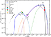 |
Fig. A.1. Representative attempt of single-zone leptonic model fit to the SED of PKS 0346-27 during the H.E.S.S. detection night of 3 November 2021. The individual radiation components are shown without EBL absorption, adding up to the total intrinsic model SED shown by the solid blue curve. The solid black line shows the total model curve accounting for EBL absorption following the Finke et al. (2010) model. The archival flux points are from https://tools.ssdc.asi.it/SED/. We refer to Table A.1 for model parameters. |
Parameters for the representative leptonic-model fit attempt to the detection-night SED shown in Fig. A.1.
While, in principle, a satisfactory SED fit is possible with this setup, the required choices of parameters is extreme: In particular, the system is more than 5 orders of magnitude out of equipartition (particle dominated), which poses problems of particle confinement and the source of energy powering particle acceleration. Also, the magnetic field of 48 mG is much lower than what is usually found in SED modelling of FSRQ-type blazars and the large Doppler and bulk Lorentz factor of 80 appear uncomfortably high, although such values have been inferred from radio observations in a few cases. We therefore conclude that a single-zone leptonic model is disfavoured compared to the hadronic model fit presented in the main text, which could be achieved with much more natural parameter choices.
All Tables
Very high energy γ-ray spectral parameters for the detection night of 3 November 2021.
Parameters for the representative leptonic-model fit attempt to the detection-night SED shown in Fig. A.1.
All Figures
|
Fig. 1. Result for θ2 from the 3 November 2021 (MJD 59521.93 – 59521.99) observation night analysis and significance plots with the four selected runs. Top-left and bottom-left panels: Results from the CT1-4 dataset. Top-right and bottom-right panels: Results from the CT5 dataset. The inset shows the point spread function, which was derived by fitting the θ2 distribution to the KING’s function, described in Ackermann et al. (2013). |
| In the text | |
|
Fig. 2. Observed spectra and flux points together with intrinsic flux points for the CT1-4 (top panel) and CT5 (bottom panel) dataset. The observed spectrum and flux points were de-absorbed with the Finke et al. (2010) EBL model. The orange bands are the statistical errors only, while the purple bands show the systematic errors together with the statistical errors. The error bars of the flux points are statistical only. |
| In the text | |
|
Fig. 3. Multi-wavelength light curves from MJD 59515.99 – 59526.10. Panels from top to bottom: H.E.S.S flux for CT1-4 and CT5 in 10−11 cm−2 s−1, Fermi-LAT flux for both 12-h and 24-h binning in 10−6 cm−2 s−1, Fermi-LAT spectral index for 24-h binning, Swift-XRT flux in 10−12 erg cm−2 s−1, Swift-UVOT flux in 10−12 erg cm−2 s−1, and ATOM flux for V, B and R filters in 10−12 erg cm−2 s−1. The double vertical dotted red lines denote the H.E.S.S. detection period, MJD 59521.93 – 59521.99. Only statistical errors are shown. |
| In the text | |
|
Fig. 4. Spectral energy distribution of PKS 0346-27 during the H.E.S.S. detection night of 3 November 2021 fit with a hadronic single-zone model. The individual radiation components are shown without EBL absorption, and they add up to the total intrinsic model SED shown by the solid blue curve. The solid black line shows the total model curve accounting for EBL absorption following the Finke et al. (2010) model. The Fermi-LAT emission is explained by the proton-synchrotron component while the casacade component explains the H.E.S.S. emission. The archival flux points are from https://tools.ssdc.asi.it/SED/. We refer to Table 2 for model parameters. |
| In the text | |
|
Fig. A.1. Representative attempt of single-zone leptonic model fit to the SED of PKS 0346-27 during the H.E.S.S. detection night of 3 November 2021. The individual radiation components are shown without EBL absorption, adding up to the total intrinsic model SED shown by the solid blue curve. The solid black line shows the total model curve accounting for EBL absorption following the Finke et al. (2010) model. The archival flux points are from https://tools.ssdc.asi.it/SED/. We refer to Table A.1 for model parameters. |
| In the text | |
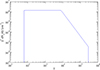 |
Fig. A.2. Radiating electron spectrum from the leptonic SED fit shown in Fig. A.1. |
| In the text | |
Current usage metrics show cumulative count of Article Views (full-text article views including HTML views, PDF and ePub downloads, according to the available data) and Abstracts Views on Vision4Press platform.
Data correspond to usage on the plateform after 2015. The current usage metrics is available 48-96 hours after online publication and is updated daily on week days.
Initial download of the metrics may take a while.