| Issue |
A&A
Volume 706, February 2026
|
|
|---|---|---|
| Article Number | A222 | |
| Number of page(s) | 12 | |
| Section | Planets, planetary systems, and small bodies | |
| DOI | https://doi.org/10.1051/0004-6361/202557279 | |
| Published online | 13 February 2026 | |
ExoNAMD: Leveraging the spin–orbit angle to constrain the dynamics of multi-planet systems
1
Dipartimento di Fisica, La Sapienza Università di Roma,
Piazzale Aldo Moro 5, Roma
00185,
Italy
2
INAF – Osservatorio Astrofisico di Arcetri,
Largo Enrico Fermi 5,
50125
Firenze,
Italy
3
Astronomical Institute of the Czech Academy of Sciences,
Fričova 298, 25165 Ondřejov,
Czech Republic
4
INAF – Osservatorio Astrofisico di Torino,
Via Osservatorio 20, 10025 Pino Torinese,
Italy
★ Corresponding author: This email address is being protected from spambots. You need JavaScript enabled to view it.
Received:
16
September
2025
Accepted:
3
December
2025
Abstract
Multi-planet systems are excellent laboratories for studying the formation and evolution of exoplanets inside the same stellar environment. The number of known multi-planet systems is expected to skyrocket with the advent of PLATO and the Roman space telescope. The spin–orbit angle is a key context information for the systems’ dynamical history, and in recent years a growing number of planets had their spin–orbit angles measured, revealing a large diversity in orbital configurations, from well-aligned to polar, and even retrograde, orbits. Still, observers lack a robust tool with which to compare the dynamical state of different systems and to select the most suitable ones for future avenues of exploration, such as investigating the evolutionary pathways and their links to the atmospheric composition. Here, we present ExoNAMD, an open source code aimed at evaluating the dynamical state of multi-planet systems via the Normalized Angular Momentum Deficit (NAMD) metric. The NAMD measures the deficit in angular momentum with respect to circular, co-planar orbits. It is normalized to compare systems with different architectures and provides a lower limit on the past dynamical excitation of the system. We find that using the spin–orbit angle parameter in the NAMD calculation (A-NAMD) improves the dynamical state’s description, compared to using only the relative inclinations (R-NAMD). Comparison of A-NAMD and R-NAMD also yields powerful insights into the interplay between eccentricity and spin–orbit angle. ExoNAMD is a timely tool for easy and fast comparison of the myriad of exoplanetary systems to be discovered by PLATO and Roman and to optimize the target selection and scientific output for future atmospheric characterization using ELTs, JWST, and Ariel.
Key words: celestial mechanics / planets and satellites: atmospheres / planets and satellites: dynamical evolution and stability / planet-star interactions
© The Authors 2026
 Open Access article, published by EDP Sciences, under the terms of the Creative Commons Attribution License (https://creativecommons.org/licenses/by/4.0), which permits unrestricted use, distribution, and reproduction in any medium, provided the original work is properly cited.
This article is published in open access under the Subscribe to Open model. This email address is being protected from spambots. You need JavaScript enabled to view it. to support open access publication.
1 Introduction
The discovery of about 6000 exoplanets in nearly 30 years has revolutionized our understanding of planets and planetary systems, previously based on the sole example of the Solar System. The discoveries reveal a vast diversity of physical and orbital properties of planets around different stellar types, from hot Jupiters to super-Earths, and from around B-type stars to brown dwarfs and even pulsars. Recently, the emphasis in the field has shifted from discovery to detailed characterization. The parameter space to characterize, however, is multidimensional, posing a significant challenge to the achievement of a unified theory for planetary formation and evolution histories, as for stars.
Constraining the origins of individual exoplanets is a challenging task as different formation and migration histories can result in the same observed outcome (Dawson & Johnson 2018). For example, the migration pathways of hot and warm Jupiters are still debated, with the contribution of gas-disk migration (Ida & Lin 2004; Baruteau et al. 2014) versus high-eccentricity migration via the Kozai–Lidov mechanism (Fabrycky et al. 2014) still unconstrained by observations. In this context, multi-planet systems are crucial case studies, as their planets formed and migrated in the same stellar environment.
The observed population of multi-planet systems (∼ 1000 known systems) shows a great diversity (Mishra et al. 2023) covering a range of eccentricities, masses, orbital periods, and spin–orbit angles. No individual parameter nor single combination of parameters (metric) is sufficient to capture this diversity; specialized metrics need to be developed to homogeneously compare the properties of different systems, constrain their formation pathways, and select the most suitable for follow-up observations. The ultimate goal is to have a comprehensive theory of planets and how they formed and evolved that allows us to assess the uniqueness of our own Solar System and conditions for life elsewhere in the Galaxy.
There are two main methods for investigating the histories of planetary systems based on their present properties. The first is the spectroscopic characterization of exoplanetary atmospheres (Tinetti et al. 2013; Madhusudhan 2019; Turrini et al. 2022) that carry information about their formation and subsequent evolution. The interpretation of spectroscopic data to constrain the planetary histories must account for how the atmospheric composition of planets can change over time. Atmospheres connect the planet to its host star, as their upper layers are shaped by the stellar environment, which alters the composition via photochemistry (Fortney et al. 2020; Tsai et al. 2023). In multi-planet systems, planetesimal bombardments and planetary collisions can alter or cancel the original signatures of planet formation (Turrini et al. 2015; Seligman et al. 2022; Sainsbury-Martinez & Walsh 2024; Polychroni et al. 2025). Furthermore, multi-planet systems are excellent laboratories in which to test how these processes alter the original composition as a function of the orbital distance (Barat et al. 2024). The advent of the JWST has transformed our view of exoplanetary atmospheres, shifting the field from detection of individual chemical species and partial classification to detailed characterization. Outstanding results include the robust detection of major trace gases such as CO2, H2 O, and CH4, as well as photochemically produced SO2 (Rustamkulov et al. 2023; Tsai et al. 2023; Powell et al. 2024). JWST successes also highlight three critical challenges and opportunities that the exoplanetary community will face in the next decades: (i) selecting optimal targets for detailed spectroscopic characterization with existing and future instrumentation; (ii) compiling unbiased target lists for large spectroscopic survey missions such as Ariel; (iii) correctly interpreting the atmospheric data (e.g., three key criteria; Seager et al. 2025).
The second method to investigate planetary systems’ histories is to characterize the architectures of the systems through the physical and orbital parameters of the planets and their host star (e.g., Turrini et al. 2022; Leleu et al. 2024). Among these parameters, the spin–orbit angle1 (the physical equivalent of the absolute orbital inclination in celestial mechanics) has emerged in recent years as a powerful probe of the dynamical history. It is defined as the angle between the stellar spin axis and the normal to the orbital plane of the planet (Albrecht et al. 2022). The spin–orbit angle is a physical property intrinsic to each planet, unlike the inclination with respect to the celestial sphere, which depends on the line of sight. Recent measurements of spin–orbit angles have revealed an unexpectedly wide variety of orbits, from well-aligned to polar and even retrograde ones. Also in this case, multi-planet systems offer a unique opportunity to study the phenomena behind these diverse architectures, dictated by the delicate interplay of multiple processes such as the Kozai–Lidov mechanism, secular resonances, mean-motion resonances, planet-planet scattering, and eccentricity cascade.
These two methods are complementary, each revealing different aspects of the nature of planets. Only by leveraging their combined usage can we overcome their individual limitations in constraining the planetary systems’ histories.
This work focuses on the second method and aims to construct robust metrics and diagnostic tools to characterize the dynamics of planetary systems and allow cross-system comparisons. Previous works (Laskar 1997, 2000; Laskar & Petit 2017) introduced the Angular Momentum Deficit (AMD) metric – which measures the deviation of planetary orbits from the circular and co-planar case – to study the dynamical stability of the Solar System and later exoplanetary systems. The focus of the AMD is on constraining the future stability of the systems. The AMD offers a computationally efficient method, requiring no numerical integration and relying solely on derived orbital parameters. However, AMD does not provide a timescale for potential instability and neglects important dynamical phenomena such as mean-motion resonances, which can significantly influence system behavior.
In parallel to AMD, several other metrics have been developed to predict the future stability of planetary systems to address the limitations of the AMD metric. These include MEGNO (Mean Exponential Growth of Nearby Orbits, Cincotta & Simó 2000) and SPOCK (Stability of Planetary Orbital Configurations Klassifier, Tamayo et al. 2020), each with distinct advantages and drawbacks.
The MEGNO metric evaluates stability through numerical integration and chaos indicators, capturing intricate dynamical interactions and providing direct physical insights. However, MEGNO is computationally intensive and typically integrates systems over a limited number of orbits, potentially overlooking long-term dynamical trends. In contrast, SPOCK leverages machine learning trained on extensive numerical simulations to quickly predict whether planetary systems are dynamically stable or unstable. Although SPOCK offers rapid stability assessments without the computational expense of numerical integration, it relies heavily on pre-trained datasets and lacks the direct interpretability provided by MEGNO or AMD. Also, SPOCK is designed only for systems with three or more planets, limiting its applicability. Recent studies (e.g., Gajdoš & Vaňko 2023) have utilized these stability metrics to assess the future stability of planetary systems and compare their predictive capabilities.
Building upon AMD, and focusing instead on the past dynamical histories, Chambers (2001, hereafter CH1) and Turrini et al. (2020, T20) developed the Normalized Angular Momentum Deficit (NAMD) metric, which allows for homogeneous quantitative comparisons of dynamical excitation across different multi-planet systems, regardless of their specific orbital architectures. The NAMD normalization eliminates the dependency on the planetary masses and semi-major axes, overcoming the limitation of the AMD, which could not compare systems with compact (e.g., TRAPPIST-1, Gillon et al. 2017) and extended architectures (e.g., HR 8799; Marois et al. 2010). The interpretation of the NAMD is straightforward: higher NAMD values indicate greater dynamical excitation and higher probabilities of past dynamical instabilities, making NAMD an effective “thermometer” for evaluating the past dynamical history of planetary systems (Turrini et al. 2022, hereafter T22).
While qualitative information on multi-planet systems can be derived from basic considerations on their orbital properties – for example, whether the planetary eccentricities cause the orbits to intersect or whether the planets have very different spin–orbit angles – this approach does not allow for homogeneous and quantitative comparisons between systems with different architectures. As an example, this approach does not allow us to easily assess whether a planetary system containing two Saturn-mass planets on eccentric orbits is more or less excited than a system containing a Jupiter-mass planet on a more mildly eccentric one. By tying the dynamical excitation of planetary systems to their angular momentum – hence, weighting eccentricity and inclination by the mass and semimajor axis of the planets – the NAMD naturally allows for this kind of homogeneous quantitative comparison (Turrini et al. 2020, 2022). Moreover, in combination with metrics such as AMD, MEGNO, and SPOCK, it allows for the complete description of the past, present, and future dynamical states of planetary systems.
The formulation of the NAMD by T20 uses the relative inclination with respect to the most massive planet in the system as a proxy of the spin–orbit angle. However, the NAMD in this formulation does not consider orbital misalignment with the stellar spin axis, which is captured in the spin–orbit angle parameter, ψ. For instance, without this key parameter, the NAMD cannot capture the difference in the dynamical state of two systems with transiting planets: one characterized by planets on aligned orbits (orbiting in the same direction as the stellar rotation), and one with planets on polar or even retrograde orbits. The latter is characterized by a higher degree of dynamical excitation.
The original NAMD formulation by T20 was well justified with the small number of spin–orbit angle measurements available at the time. However, with the advancement of highresolution spectrographs (Schwab et al. 2016; Pepe et al. 2021; Seifahrt et al. 2022), Rossiter-McLaughlin (R-M) effect measurements have increased dramatically in number and quality since T20 (Knudstrup et al. 2024; Espinoza-Retamal et al. 2025; Zak et al. 2025b), thus increasing the number of planets for which we have the spin–orbit angle measured to the point where an updated NAMD formulation is warranted.
Currently, the projected spin–orbit angle is known for more than 300 planets, and out of those around 10% are in multi-planet systems. This parameter is the spin–orbit angle projected onto our line of sight. On the other hand, the de-projected spin–orbit angle (hereafter, spin–orbit angle), is known for about 150 planets, and around 15% of those are in multi-planet systems. With the upcoming launch of the PLATO space mission (Rauer et al. 2025), the stellar inclination of a large number of stars will be measured thanks to its long-term observing strategy. This, combined with dedicated ground-based follow-ups2 providing the projected spin–orbit angle (e.g., Zak et al. 2025c), will lead to even faster growth in spin–orbit angle measurements.
We updated the relative inclination-based NAMD formulation by T20 (hereafter R-NAMD) by replacing the relative inclination with respect to the most massive planet in the system with the spin–orbit angle parameter, which gives the spin–orbit angle-based NAMD (hereafter, A-NAMD). The number of spin–orbit angle measurements is still limited as they are observationally expensive, and hence the R-NAMD remains a viable tool for characterizing the dynamics of the exoplanetary population. Furthermore, as we present in this paper, the R-NAMD and A-NAMD metrics can be used jointly to increase their diagnostic power and derive more detailed constraints on the orbital dynamics.
To directly support the community, we implemented both the R-NAMD and A-NAMD calculations in an open-source Python tool, ExoNAMD3. The dynamical context provided by the NAMD enables (1) cross-system dynamical-state comparisons; (2) unbiased target selection for future observations; (3) comprehensive dynamical descriptions alongside stability metrics (AMD, MEGNO, SPOCK) in the forthcoming era of PLATO and Ariel, and (4) the interpretation of measurements of planetary atmospheres, as migration history shapes their composition and thermal structure.
2 Methods
2.1 NAMD
The general formulation of the NAMD defined in CH1 and T20 is
 (1)
where mk is the mass of the k th planet, ak its semimajor axis, ek its eccentricity, and ik its inclination. As discussed in T20, the NAMD measures the dynamical excitation of planetary systems, which is tied to the occurrence and intensity of dynamical instabilities, hence the “violence” of the dynamical evolution (T20, T22). The in-plane excitation appears in the NAMD through the orbital eccentricities, while the out-of-plane excitation appears through the inclinations.
(1)
where mk is the mass of the k th planet, ak its semimajor axis, ek its eccentricity, and ik its inclination. As discussed in T20, the NAMD measures the dynamical excitation of planetary systems, which is tied to the occurrence and intensity of dynamical instabilities, hence the “violence” of the dynamical evolution (T20, T22). The in-plane excitation appears in the NAMD through the orbital eccentricities, while the out-of-plane excitation appears through the inclinations.
In the case of exoplanetary systems, however, the inclination of the planets is referred to the local plane of the celestial sphere and not to a physically meaningful plane. In the original study by CH1, focused on the formation of the inner Solar System, the inclinations ik were implicitly assumed as referring to the midplane of the Solar Nebula. To circumvent this issue when the spin–orbit angles are unknown, Zinzi & Turrini (2017) and Turrini et al. (2020) introduced the approach of adopting the orbital plane of the most massive planet in the system as the reference plane, based on the reasoning that this planet was plausibly the least excited and, therefore, the one closer to the original disk midplane. This approach led to the formulation of the relative NAMD (R-NAMD), defined in T20 as
 (2)
where ir, k is the inclination of the k th planet with respect to the most massive planet in the system. The out-of-plane excitation in the R-NAMD is a lower limit to the real one, given that ir, k underestimates the true spin–orbit angles and the impact of specific viewing geometries (e.g., if the line of nodes is along the line of sight). Thus, the R-NAMD provides a lower limit to the dynamical excitation of the system.
(2)
where ir, k is the inclination of the k th planet with respect to the most massive planet in the system. The out-of-plane excitation in the R-NAMD is a lower limit to the real one, given that ir, k underestimates the true spin–orbit angles and the impact of specific viewing geometries (e.g., if the line of nodes is along the line of sight). Thus, the R-NAMD provides a lower limit to the dynamical excitation of the system.
In this work, we expanded the application of the NAMD methodology to exoplanetary systems by introducing the absolute NAMD (A-NAMD) by replacing ik and ir, k with the spin–orbit angle, ψk, which gives
 (3)
(3)
The expression is divided by two to ensure that A-NAMD values are normalized to one. The individual parameters needed for the R-NAMD and A-NAMD computation are briefly explained in Appendix A, together with the most widely-used techniques to obtain them. The A-NAMD provides a representative estimate of both in-plane and out-of-plane dynamical excitation. When the spin–orbit angle is known for only one planet in the system, this information can be used in principle to extrapolate the spin–orbit angles, ψr, k, relative to the plane perpendicular to the stellar spin axis from the relative inclinations of the planets. As in the case of R-NAMD, however, this approach does not account for the impact of specific viewing geometries of the orbits.
The NAMD metric is a temporally evolving quantity, as tidal forces can realign and circularize the orbits, lowering the dynamical excitation over time. This is true for both the R-NAMD and A-NAMD formulations. In Sect. 4, we discuss the relevant timescales for orbital circularization and realignment in the context of the R-NAMD and A-NAMD metrics.
2.2 ExoNAMD: A community tool
To date, there is no open-source tool available for the community to compute the NAMD, in either form. Hence, to fill this gap and streamline the preparation of follow-ups of multi-planet systems, we present a new community tool called ExoNAMD, which we used for the analyses in this study.
ExoNAMD is a user-friendly Python 3.8+ code that computes both the R-NAMD and A-NAMD and associated uncertainties, enabling quick and efficient comparisons of the remaining dynamical violence in the architecture of multi-planet systems. The code is extensively documented on Read the Docs 4, including examples and guides. ExoNAMD is available on PyPI5 for installation via
$ pip install exonamd
The steps to compute the NAMD are listed below.
Retrieve the planet’s parameters, either from the NASA Exoplanet Archive 6 or parsing a user input .csv file.
Input any missing parameters and uncertainties (see the code documentation and/or Appendix B).
Assess the variability of the parameters via Monte Carlo methods using their uncertainties.
Compute the NAMD using the spin–orbit angle (A-NAMD) or the relative inclination with respect to the most massive planet (R-NAMD).
The R-NAMD offers insights on the systems’ dynamics when the spin–orbit angle is not available. The A-NAMD allows for a more complete characterization of the system’s dynamical state, as it takes into account its true architecture. The following section includes examples (such as K2-290 and Kepler-462) where only the inclusion of the ψ parameter enables the correct interpretation of the system’s architecture and possible planetary evolutionary pathways.
2.3 Building the sample
Here, we describe the steps taken to obtain the sample of planetary systems we analyze in the following section. All these steps are natively implemented in ExoNAMD.
We queried the NASA Exoplanet Archive for all multi-planet systems and retrieved 1 005 unique multi-planet systems (date: 7 August, 20257). We created a database of aliases for the removal of duplicates. We solved for missing values of stellar mass, orbital period, or semimajor axis using the third Kepler law if any two parameters of this set of three were available. We also solved for the stellar radius or the semimajor axis if the database reports only their ratio, and similarly for the stellar radius and the planetary radius. For each planet, we took the median value from all queried values and their uncertainties obtained from the NASA Exoplanet Archive to avoid biases and outliers in the subsequent analysis, discarding any NaNs. Then, we cleaned our sample by discarding duplicate systems using our database of aliases, obtained using a custom catalogue implementation available in ExoNAMD, which is inspired by the gen_tso code (Cubillos 2024). In the event that some of the parameters are not available, ExoNAMD offers the possibility to interpolate their values (see Appendix B for details).
Following the methodology in T20, we computed both the R-NAMD and A-NAMD together with their uncertainties using a Monte Carlo approach. We used the truncnorm function from scipy.stats, and we drew 100 000 random samples from a truncated normal distribution within the physical bounds of each parameter (e.g., nonnegative masses). The distribution is centered at the obtained value from the previous steps, and its half-width was obtained from the arithmetic mean of the upper and lower error bars. We performed this step on all parameters needed for the R-NAMD and A-NAMD calculations in Eqs. (2) and (3). We took the median of the final distribution as the expected NAMD value, with associated uncertainties from the 16th-84th percentile. Finally, we computed the relative uncertainty on the NAMD following T20: we took the half interquartile range and normalized it by the median. This allowed us to keep track of the cases with too high a relative uncertainty (higher than unity) when we interpreted the results. We also included the Solar System in the analysis as a reference point using the values reported on the NASA Planetary Fact Sheet 8 following T20 and T22.
3 Results
After performing the above steps, we were left with 792 multi-planet systems, including those with interpolated values. Following T20, we decided to restrict our sample to systems for which we have all the parameters for the R-NAMD calculation (without interpolations) to avoid possible biases. We refer to this as the “core” sample, and it consists of 67 systems. The multiplicity distribution in the core sample is as follows:
45 systems with M=2
eight systems with M=3
seven systems with M=4
two systems with M=5
three systems with M=6
one system with M=7 (TRAPPIST-1)
one system with M=8 (the Solar System).
We show the results obtained for the R-NAMD and A-NAMD in Figs. 1 and 2. Figure 1 replicates the plot of R-NAMD versus multiplicity as in T20 (their Fig. 3), but with our expanded core sample of 67 systems versus 13 in T20.
Previous work (Limbach & Turner 2015) found an anticorrelation between the eccentricity and multiplicity of planetary systems. A subsequent study by Zinzi & Turrini (2017) linked this trend to the AMD-multiplicity trend. This result was made possible by the similar architectures of the considered systems, all of which were transiting. Thus, it was possible to directly compare across systems using the AMD metric. Finally, T20 re-observed this trend using the R-NAMD also in a larger sample of 99 systems, where missing inclinations were constrained based on the equipartition of dynamical excitation from Laskar & Petit (2017).
Figure 1 shows the same anticorrelation between the R-NAMD and multiplicity with an expanded sample. As already pointed out, the main limitation of the R-NAMD is that it does not capture the true architecture of the system, as it does not consider the spin–orbit angle. An example of how this does not capture the dynamical state of the system is provided by K2-290 and Kepler-462, which we analyze in Sect. 3.1. The R-NAMD, computed using relative inclinations between the planets, is insensitive to misalignment, and therefore it provides a lower limit to the dynamical excitation. However, as it only requires photometric data, the R-NAMD can be computed for a larger sample of systems; see Figs. 1 and 2 (spin–orbit angle data are still sparse). The knowledge of the spin–orbit angle, ψ, allows us to compute the A-NAMD, which measures the dynamical excitation corresponding to the true architecture of the planetary system.
Figure 2 shows the A-NAMD versus multiplicity. Here, we used a sample of 18 systems9, where ψ is known for the most massive planet or a planet of comparable mass. The multiplicity distribution in this sample is as follows:
ten systems with M=2
three systems with M=3
two systems with M=4
one system with M=5
one system with M=6
one system with M=8 (the Solar System).
Finally, a trade-off between the number of characterized systems and the accurate physical description of their dynamical state can be reached by using the projected spin–orbit angle, λ, instead of ψ in Eq. (3), which we call λ-NAMD. The advantage is that λ-NAMD does not require knowledge of the stellar inclination. The stellar inclination can be challenging to infer due to various astrophysical systematics, such as slow stellar rotation for M-dwarfs or a combination of several variability processes that can manifest, for example, in F-type stars (pulsations and ellipsoidal variations) that are over-imposed on the stellar rotation signal (Henriksen et al. 2023). The λ-NAMD can underor over-estimate the dynamical excitation, but it provides a better approximation of the true dynamical state compared to that inferred from the R-NAMD.
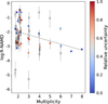 |
Fig. 1 R-NAMD versus multiplicity plot for the core sample described in the text; same as Fig. 3 in T20, but with an expanded sample. The horizontal offsets around the multiplicity values are added arbitrarily for better visualization. The color-scale, capped at one, represents the relative uncertainty on the R-NAMD values, obtained from the arithmetic mean of the lower and upper errors from the Monte Carlo method. Systems with relative uncertainty above unity are plotted with a hollow white circle. The linear fit is shown only as a visual aid as the slope is highly dependent on the (few) high-multiplicity systems. |
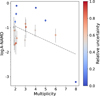 |
Fig. 2 A-NAMD versus multiplicity plot. The systems shown are selected from the core sample on the basis of the availability of spin–orbit angle measurements, as described in the text. More systems are needed to confirm and quantify the sketched anticorrelation between A-NAMD and multiplicity. The linear fit is shown only as a visual aid. |
3.1 The cases of K2-290 and Kepler-462
In the following, we compare the various NAMD metrics of two systems, K2-290 and Kepler-462, whose parameters and computed NAMD values are listed in Table 1. The K2-290 system hosts two planets on nine- and 48-day orbits (Hjorth et al. 2019). In Fig. 3, we compare the R-NAMD, A-NAMD, and λ-NAMD of this system, focusing on their respective advantages and on biases that are associated with their usage.
The R-NAMD value would be indicative of a quiescent history of the system. This is in contrast with the observed misalignment of the planetary orbits that is instead reflected in the high value of A-NAMD. This high value indicates a high degree of dynamical violence during the history of the system and hints at a chaotic past, possibly driven by the two wide-companion stars (Best & Petrovich 2022). Finally, the λ-NAMD overestimates the degree of dynamical violence by about 20% compared to the A-NAMD, as the star is not seen fully edge-on, and therefore ψ is lower than λ in this case (the qualitative information, however, is preserved).
Another instructive example is the Kepler-462 system which hosts two transiting exoplanets on well-separated but misaligned orbits (Ahlers et al. 2015). The high R-NAMD value is mostly driven by the high eccentricities. The observed misalignment further increases the dynamical violence of the system and is reflected in the still higher A-NAMD. In this system, the λ-NAMD is 2.5 times lower than the A-NAMD (although it is consistent with the A-NAMD within 3 σ). Similarly to K2-290, the difference between the R-NAMD and A-NAMD is critical and highlights the usefulness of the A-NAMD to capture the true architecture of the system in an unbiased manner (see Fig. C.1).
3.2 A new diagnostic: The four-quadrant diagram
The A-NAMD metric introduced in this paper connects the information concerning the eccentricity and spin–orbit angle (or “absolute inclination”). Both parameters provide a record of the dynamical state of the system (T22) and are closely linked by the energy-equipartition theorem (Laskar & Petit 2017; He et al. 2020). Several mechanisms are responsible for exciting the planetary eccentricities and/or the spin–orbit angles, and their effect over time is manifested in the observed parameter space. So, by studying the distribution of the relevant dynamical parameters and comparing them to theoretical model predictions, we can attempt to identify (i) possible trends that emerge from these complex dynamical interactions, (ii) the most common evolutionary pathways, and (iii) the relative contributions of each pathway to the observed population. Ideally, these studies should be complemented by independent information from atmospheric studies that can reveal additional details and identify anomalies and knowledge gaps.
An example of a dynamical process where eccentricities and spin–orbit angles are tightly linked is high-eccentricity migration coupled with the Kozai–Lidov (KL) mechanism (Fabrycky & Tremaine 2007). In the KL mechanism, planets undergo periodic exchanges of eccentricity and spin–orbit angle with a third, distant massive object and move inward toward the host star thanks to tidal forces. Another example which provides testable predictions is the formation of ultra-short-period (USP) planets. Millholland & Spalding (2020) suggested that USP planets should be aligned with the stellar spin axis; however, they should be misaligned with respect to the exterior planets. Recently, Yang et al. (2025) suggested a new mechanism to explain the production of eccentric and highly misaligned hot Jupiters: the “eccentricity cascade”. This mechanism involves an outer companion star that induces eccentricity oscillations in the inner companion star through the KL mechanism, and these excitations are transferred to the planet through close encounters, triggering its migration toward the star. Between close encounters, the orbits evolve through secular diffusion (Laskar & Petit 2017; He et al. 2020).
When discussing the interplay of eccentricities and spin–orbit angles, we refer to systems characterized by eccentric orbits as “excited” and systems characterized by misaligned orbits as “perturbed” for reasons that we clarify in the following. To quantify the prevalence of excitation and perturbation, we introduce a new diagnostic tool in the form of a diagram of A-NAMD versus R-NAMD. Figure 4 reports an example of this diagram, built with the 18 systems including the Solar System used in Fig. 2, and nine synthetic systems10 to populate the figure.
Following T22, we used the Solar System values a dividing point in the diagram. The Solar System lies on the boundary between systems with orderly and chaotic evolution (Nesvorný 2018). We also include a Solar System perturbed by 15 degrees as an illustration to account for a possible primordial misalignment during planet formation (Takaishi et al. 2020). Additionally, we include a yellow horizontal region between the Solar System, and its version perturbed by 15 degrees. In this uncertainty region, planetary systems could be either perturbed or excited. Moreover, based on results from Rickman et al. (2023), we introduced another uncertainty region that extends vertically from half the R-NAMD of the Solar System to twice its value. Here, systems may or may not be excited.
The usage of the Solar System allows us to visually separate the following four quadrants:
Top left: perturbed but non-excited systems, characterized by high A-NAMD and low R-NAMD values. These systems have misaligned orbits with low eccentricity, which could be indicative of past gravitational interactions that were more effective in the vertical direction, or stellar encounters that affected the disc before planets formed. In this quadrant, systems with short orbits might have had their orbits circularized but not yet realigned.
Top right: perturbed and excited systems, described by high A-NAMD and R-NAMD values. This is indicative of eccentric and misaligned orbits hinting at past gravitational encounters and highly violent dynamical history, possibly coupled with the KL mechanism or eccentricity cascade. Such systems are more likely to contain a distant companion on a wide orbit that might be responsible for the chaotic history or have undergone a stellar encounter that destabilized the system.
Bottom left: non-perturbed and non-excited systems with low A-NAMD and R-NAMD values. These systems have likely experienced quiescent evolution, likely through disk migration, and were not altered by instability processes. For compact systems on short orbits, it is also plausible that their entire dynamical history has been erased through tidal forces.
Bottom right: non-perturbed but excited systems have low A-NAMD and high R-NAMD values. This is indicative of eccentric and well-aligned orbits. This configuration can be reached by gravitational interactions that are more effective in the planar direction. For example, a distant companion that keeps a low but nonzero eccentricity of an inner companion without misaligning the orbits, or planet-planet scattering in a highly coplanar system.
These quadrants are further discussed in the next section, with a focus on current observational biases.
Parameters of K2-290 and Kepler-462 systems.
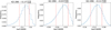 |
Fig. 3 Comparison of NAMD values for the K2-290 system. The system consists of two planets on highly misaligned orbits. Left: R-NAMD as defined in T20 using relative inclinations. Middle: λ-NAMD, using the projected spin–orbit angle (λ). Right: A-NAMD as defined in this work using the spin–orbit angle (ψ). The A-NAMD is the most suitable to capture the true architecture of the system as it is not affected by projection effects. |
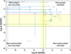 |
Fig. 4 Four-quadrant diagram. This figure illustrates the possible states in which planetary systems can be found depending on their dynamical history, which is reflected in their eccentricities and spin–orbit angles. The Solar System is located at the intersection of the two gray dashed lines and separates the four quadrants, as discussed in the text. As an illustration, we include a value (red line) of a Solar System with planets misaligned by 15 degrees. The vertical highlighted area marks instead the R-NAMD values that can be associated with excited but stable systems that did not undergo large-scale instabilities in the simulations by Rickman et al. (2023). In addition, we included several synthetic systems based on real ones for which some parameters were missing (green points). These were inputted in order to better populate the quadrants. |
4 Discussion
We introduced the four-quadrant diagram as a new diagnostic tool for distinguishing the prevalence of excitation and perturbation in the dynamical states of planetary systems. However, the interpretation of the four quadrants in Fig. 4 needs additional context concerning possible observational biases that affect the currently observed population of exoplanets. Here, we summarize the main ones:
The upper quadrants are currently over-populated. This is due to the error bars on ψ being on average 20 times larger compared to the median value of relative planetary inclinations for transiting exoplanets. These large error bars drive up the A-NAMD values when using the Monte Carlo method explained before. However, with advances in instrumentation (Seifahrt et al. 2018; Pepe et al. 2021), the ψ parameter can be constrained to less than one degree (e.g., Casasayas-Barris et al. 2017; Watanabe et al. 2024; Rubenzahl et al. 2024) with ultra-precise spectrographs, effectively correcting this bias.
Upper left quadrant. Old, compact systems will be over-represented in this quadrant as tidal forces act on faster timescales for orbit circularization compared to orbit realignment (Bonomo et al. 2017). This results in a faster right-left movement than a top-bottom one.
Lower left quadrant. Only transiting planets (low relative inclinations) are suitable for spin–orbit angle measurements via the R-M effect, which provided the bulk of spin–orbit angle measurements so far. Thus, there is an observational bias leading to over-representation of systems in this diagram compared to having a statistical sample of the general exoplanet population. However, this quadrant contains very few systems. One reason might be that the bias in point 1 is depopulating this quadrant, and this issue can only be mitigated with more precise measurements of the spin–orbit angle.
Another bias affecting the NAMD is the possibility of primordial misalignment. Recent works (e.g., Kuffmeier et al. 2024) have suggested that primordial misalignment can produce misaligned orbits by more than 15−20 deg, as originally suggested by Takaishi et al. (2020). This creates an uncertainty region for the interpretation of the A-NAMD. A similar uncertainty region to that mentioned in point 4 also affects the interpretation of R-NAMD, as it is unclear what the minimum excitation created by instabilities is (Turrini et al. 2022; Rickman et al. 2023).
As mentioned in the second point, tidal dissipation can severely affect the derived NAMD values. Hence, computing the dynamical timescales (circularization and realignment timescales; Goldreich & Soter 1966; Adams & Laughlin 2006) can be used to constrain and better interpret the observed position and possible movements across the four-quadrant diagram. This in turn can be used to correct the occurrence rates of planetary instabilities and star-triggered effects.
Tidal forces act on various timescales11 on the spin orbit angle and planetary eccentricities, and affect the innermost planets more significantly. Therefore, the effect of tidal forces is most relevant for systems with planets on short-period orbits around cool stars with convective envelopes, for which the tidal forces are more efficient. Notably, the distribution of the spin–orbit angle for hot Jupiters is shaped both by gravitational and tidal effects (Anderson et al. 2021; Spalding & Winn 2022). An illustrative example is provided by the shortest period hot Jupiter in our sample of systems discussed in Fig. 2: WASP-47 b. The timescales for the circularization and the realignment of its orbit would be between 0.1 and 1 Gyr (depending on the tidal quality factor) and 1000 Gyr, respectively. Compared to the age of the system of ∼ 6−7 Gyr (Almenara et al. 2016), the planetary eccentricity has been likely affected since its formation by the tidal forces, while the spin–orbit angle has not. So, we recommend that a comparison between the dynamical timescales and the age of the star be made, especially for planets on short-period orbits, to assess whether the dynamical information has been diluted over time (Harre et al. 2024). This is crucial in order to check for possible biases in the interpretation of the NAMD values when searching for population-level trends.
4.1 Planetary atmospheres
A distinct and complementary probe of the dynamical state is the composition of planetary atmospheres, which can help reveal past evolution even when the NAMD information is biased. Planetary atmospheres are unique windows into the interior compositions of planets, which hold the record of how and where they formed (Öberg et al. 2011; Turrini et al. 2021; Schneider & Bitsch 2021). At the same time, they connect the planet to its host star and are shaped by the stellar environment. Therefore, multi-planet systems under the same stellar environment offer us opportunities to test planetary evolution and migration theories, such as the link between migration and composition or the formation of compact architectures (Pacetti et al. 2022). Specifically, the derived elemental ratios such as C/O, C/N, N/O, and S/N from spectroscopic measurements of exoplanet atmospheres can help us distinguish among various planetary migration scenarios (Turrini et al. 2021; Crossfield 2023), as they are strongly dependent on the initial semimajor axis of the planet orbit.
Several mechanisms can alter the signatures of the different migration pathways (Dawson & Johnson 2018). For instance, tidal forces can realign the originally misaligned planet. Or, the originally aligned planet can later be misaligned by some additional mechanisms (e.g., internal gravity waves, Rogers et al. 2013). To an extent, studying the atmospheric composition can lift the veil on previous history. Another example of the atmosphere-dynamics connection was presented in Sethi & Millholland (2025). The authors found that misaligned planets tend to be more inflated (through tidal heating) than aligned ones, suggesting that these planets may have experienced dynamically violent processes in their past. In this context, the introduction of the A-NAMD and the four-quadrants NAMD diagram as a new diagnostic tool, as well as the open-source code ExoNAMD, will streamline the assessment of the connection between atmospheric composition and dynamical state, providing the community of observers with additional context information with which to select the most suitable targets.
This atmospheric connection to planetary dynamics is being investigated in the ongoing BOWIE-ALIGN survey (Kirk et al. 2024), which has selected a small sample of single-planet systems to follow-up with the JWST: four aligned and four misaligned planets. The main objective of this survey is the comparison of the measured atmospheric composition between dynamically active and quiescent systems, searching for possible trends to be confronted by theoretical predictions (Penzlin et al. 2024). Looking ahead, it is necessary to extend this kind of investigation to a much larger sample of systems and to include multi-planet systems to conduct comparative planetology studies in the same stellar environment. In this regard, the data from the Ariel space mission will be invaluable for studying populationlevel trends. Ariel12 aims to perform the first unbiased spectroscopic survey of hundreds of exoplanetary atmospheres in the visible and infrared (Tinetti et al. 2018). Its continuous coverage from 0.5 to 7.8 micron, observed in one shot, and excellent stability at L2 (Bocchieri et al. 2025b,a), makes it the go-to mission for large-scale, homogeneous exoplanet studies.
NAMD may also be included as a parameter in the Ariel candidate target list (Edwards & Tinetti 2022) to aid in selecting an unbiased, statistical sample of planets from a dynamical point of view. The interpretation of the Ariel observations could then be contextualized using the dynamical information provided by the NAMD (Turrini et al. 2022), as computed by our ExoNAMD tool. In this way, the results of the pathfinder BOWIE-ALIGN survey will be expanded to a statistical sample of hundreds of exoplanets, characterized homogeneously by Ariel.
The importance of having homogeneous stellar and planetary parameters has been recognized by the Ariel mission consortium as a top priority to obtain an unbiased picture of the parameter space of exoplanets. This led to the formation of various working groups. Today, all parameters needed to compute the NAMD have their respective WGs already in operation (e.g., stellar characterization WG13), including the stellar obliquity WG14, which aims to provide spin–orbit angle measurements for the majority of mission target candidates (Zak et al. 2025a) with a special focus on Tier-3 candidate targets and multi-planet systems. The ExoNAMD tool, developed within the Ariel stellar obliquity WG, is open-source and we envisage its usage by the community of observers and its adaptation to the needs of other observatories to aid in target selection and data interpretation.
4.2 Future outlook
Currently, the systems for which we possess all the needed dynamical parameters for the NAMD calculation cover only a limited portion of the parameter space of the exoplanetary population. This precludes us from having a comprehensive picture of possible shaping mechanisms, and it also makes it challenging to isolate the common processes affecting all subpopulations. Here, we comment on the ongoing and upcoming missions that will provide new windows into under-explored populations.
A currently under-explored population is that of planets on wide orbits, such as cold Jupiters. A way to isolate the effects of migration on the population of Jupiters would be to assess the dynamical excitation of hot and warm Jupiters versus cold Jupiters, as the latter migrated far less or remained close to the region of formation. The number of systems with planets on wide orbits for which the NAMD can be determined is still limited, but has seen steady growth in recent years. Thanks to astrometry and direct imaging methods (e.g., Stolker et al. 2025), we were able to increase the detection of long-period planets as well as constrain their spin–orbit angles. The upcoming DR4 Gaia release is expected to provide additional planets on wide (>1 au) orbits. While for companions at wide separations it is difficult to measure the spin–orbit angle, lower limits can be inferred by comparing the stellar rotation velocities and orbital inclinations. Bowler et al. (2023) found that companions between 10 and 250 au are consistent with having a spin–orbit angle distribution with a mixture of isotropic and aligned systems.
The PLATO mission (Rauer et al. 2025) is expected to discover between 4 600 and 24 000 exoplanets during its nominal mission depending on the assumed planetary model (Matuszewski et al. 2023). Compared to the TESS mission (Ricker et al. 2014) it is designed to yield planets on longer orbital periods (50–200 days), significantly expanding our current knowledge of the exoplanetary population. The approximately 700 multi-planet systems known from the Kepler mission (Koch et al. 2010) mostly orbit faint stars (the median magnitude is 14.5), making follow-ups rather difficult. PLATO is expected to yield at least the same number of multi-planet systems around brighter stars than those discovered by Kepler. Several ground-based, high-resolution spectrographs (e.g., PLATOSpec; Kabáth et al. 2026) will dedicate a large fraction of their available time to following up on PLATO targets with the aim of measuring their masses, eccentricities, and spin–orbit angles. Hence, the rapidly growing number of systems with measured spin–orbit angles is expected to grow even faster as well as their precision. The simultaneous photometric and spectroscopic observations can provide more precise spin–orbit angle measurements than individual spectroscopic measurements, as there are joint parameters in the light curve and the R-M effect analysis. Furthermore, multiple systems discovered by PLATO will be characterized by transit-timing variations (TTVs) with higher precision than by Kepler, thanks to the longer observation time and higher sampling rate, providing meaningful constraints to the processes of planetary formation and evolution, especially in regions of the parameter space beyond the reach of previous missions15.
Another mission relying on the TTV characterization of exoplanets is the Nancy Grace Roman Space Telescope (Akeson et al. 2019). Roman is the next NASA flagship mission that aims to detect and characterize exoplanets in the near-infrared. The predicted exoplanet yield ranges from 60 to 200 thousand transiting planetary candidates, and from 7 to 12 thousand small transiting exoplanets (Wilson et al. 2023). The main detection method will be through transit detection, but Roman is also expected to find several multi-planet systems with microlensing, further expanding the planetary parameter space to larger orbital distances (Penny et al. 2019; Fatheddin & Sajadian 2023). Most of the multi-planet systems discovered by Roman will be fainter compared to Kepler targets, and hence they will not be ideal for ground-based follow-up. Thus, the spin–orbit angle parameter will remain largely unconstrained. In the absence of a spin–orbit angle, the R-NAMD can still be used for dynamical characterization, with the caveats described before.
The next-generation, high-resolution ultra-stable instruments – including ANDES (Palle et al. 2025) at ELT, iLocater (Crepp et al. 2016) at LBT, and G-CLEF (Szentgyorgyi et al. 2016) at GMT, and many others – will significantly increase the number of spin–orbit angle measurements, covering the parameter space even of smaller planets. This will unlock the A-NAMD calculation and the dynamical assessment within the four-quadrant diagram even for planets that were previously inaccessible due to the small R-M effect amplitude or long transit durations requiring multiple instruments, for example.
5 Summary
The exoplanetary research community faces three critical challenges. First, selecting optimal targets for detailed characterization with telescopes including the JWST; second, compiling unbiased target lists for missions such as Ariel that aim to statistically explore the parameter space of the planetary population. The third challenge is correctly interpreting the atmospheric data (three key criteria, Seager et al. 2025), for which the context information on the planetary system and its evolution, including dynamical clues, is critical (T22).
To aid in addressing these challenges, this work introduces the A-NAMD metric as a powerful probe of the past dynamical histories of multi-planet systems. This metric incorporates the spin–orbit angle parameter, which has been measured for a growing number of planets in recent years, to capture the true 3D architecture of the system. For individual system studies, the A-NAMD can be used in synergy with existing stability metrics such as SPOCK, MEGNO, and AMD, which provide information on the future dynamics, whereas NAMD provides information on past behavior.
We demonstrated the diagnostic power of the joint use of the A-NAMD and the previous NAMD formulation (R-NAMD) by combining them into a four-quadrant diagram, enabling qualitative classification of systems’ dynamical histories. This diagram enables us to distinguish between the systems where dynamical events primarily affected the planar direction of the planetary orbit (producing eccentric systems) versus those where vertical effects dominated (resulting in misaligned systems). We set the Solar System, with its well-constrained parameters, as a reference point for NAMD values.
The planetary community heavily relies on the stability metrics, and their calculation is implemented, for instance, in the open-source REBOUND software (Rein & Liu 2012). These metrics concern the future stability of multi-planet systems, and our work seeks to complement them with a characterization of the past dynamical history. Despite the fact that the R-NAMD was widely adopted by the community, there is no open-source tool to calculate it. Thus, to directly support the community, we developed ExoNAMD, a user-friendly Python tool that calculates both the R-NAMD and our newly introduced A-NAMD. This open-source package features comprehensive documentation and can be installed directly from PyPI16 or GitHub17. Its flexible API allows users to easily customize calculations with their own data, for example, by adapting the example input databases given in the documentation18.
Our envisioned usage of the A-NAMD metric is to provide context information for building target lists for upcoming atmospheric missions, and facilitate optimal target selection by observers19. In this regard, we remind the reader that NAMD metrics represent a lower boundary on the intensity of past dynamical events, as processes such as tidal interactions erase evidence of past events over time. To reconstruct the complete evolutionary pathways of planetary systems, we must combine dynamical clues – for instance those provided via NAMD analysis – with detailed atmospheric composition studies. Atmospheres can preserve crucial evidence of formation and evolution processes, enabling us to develop a more complete and robust understanding of planetary systems’ histories.
Acknowledgements
A.B. and D.T. are supported by the Italian Space Agency (ASI) with Ariel grant n. 2021.5.HH.0. J.Z. acknowledges the support from GACR:22-30516K. J.Z. and D.T. acknowledge support from the COST Action CA22133 PLANETS. D.T. acknowledges support from the European Research Council via the Horizon 2020 framework program ERC Synergy “ECOGAL” project GA-855130. This research was supported by the Munich Institute for Astro-, Particle and BioPhysics (MIAPbP), which is funded by the Deutsche Forschungsgemeinschaft (DFG, German Research Foundation) under Germany’s Excellence Strategy – EXC-2094 – 390783311. We are grateful to Henri Boffin, Dominika Itrich and Pavol Gajdos for the insightful discussion improving this work.
References
- Adams, F. C., & Laughlin, G., 2006, ApJ, 649, 1004 [Google Scholar]
- Aerts, C., 2021, Rev. Mod. Phys., 93, 015001 [Google Scholar]
- Agol, E., & Fabrycky, D. C., 2018, in Handbook of Exoplanets, eds. H. J. Deeg, & J. A. Belmonte, 7 [Google Scholar]
- Ahlers, J. P., Barnes, J. W., & Barnes, R., 2015, ApJ, 814, 67 [CrossRef] [Google Scholar]
- Akeson, R., Armus, L., Bachelet, E., et al. 2019, arXiv e-prints [arXiv:1902.05569] [Google Scholar]
- Albrecht, S. H., Dawson, R. I., & Winn, J. N., 2022, PASP, 134, 082001 [NASA ADS] [CrossRef] [Google Scholar]
- Almenara, J. M., Díaz, R. F., Bonfils, X., & Udry, S., 2016, A&A, 595, L5 [NASA ADS] [CrossRef] [EDP Sciences] [Google Scholar]
- Anderson, K. R., Winn, J. N., & Penev, K., 2021, ApJ, 914, 56 [NASA ADS] [CrossRef] [Google Scholar]
- Barat, S., Désert, J.-M., Goyal, J. M., et al. 2024, A&A, 692, A198 [NASA ADS] [CrossRef] [EDP Sciences] [Google Scholar]
- Baruteau, C., Crida, A., Paardekooper, S. J., et al. 2014, in Protostars and Planets VI, eds. H. Beuther, R. S. Klessen, C. P. Dullemond, et al. 667 [Google Scholar]
- Best, S., & Petrovich, C., 2022, ApJ, 925, L5 [NASA ADS] [CrossRef] [Google Scholar]
- Bocchieri, A., Booth, L., & Mugnai, L. V. 2025a, Exp. Astron., 60, 19 [Google Scholar]
- Bocchieri, A., Mugnai, L. V., Pascale, E., et al. 2025b, Exp. Astron., 59, 31 [Google Scholar]
- Bonomo, A. S., Desidera, S., Benatti, S., et al. 2017, A&A, 602, A107 [NASA ADS] [CrossRef] [EDP Sciences] [Google Scholar]
- Bourrier, V., Lovis, C., Cretignier, M., et al. 2021, A&A, 654, A152 [NASA ADS] [CrossRef] [EDP Sciences] [Google Scholar]
- Bowler, B. P., Tran, Q. H., Zhang, Z., et al. 2023, AJ, 165, 164 [NASA ADS] [CrossRef] [Google Scholar]
- Campante, T. L., Lund, M. N., Kuszlewicz, J. S., et al. 2016, ApJ, 819, 85 [Google Scholar]
- Casasayas-Barris, N., Palle, E., Nowak, G., et al. 2017, A&A, 608, A135 [NASA ADS] [CrossRef] [EDP Sciences] [Google Scholar]
- Chambers, J. E., 2001, Icarus, 152, 205 [Google Scholar]
- Cincotta, P. M., & Simó, C., 2000, A&AS, 147, 205 [NASA ADS] [CrossRef] [EDP Sciences] [Google Scholar]
- Crepp, J. R., Crass, J., King, D., et al. 2016, SPIE Conf. Ser., 9908, 990819 [Google Scholar]
- Crossfield, I. J. M., 2023, ApJ, 952, L18 [NASA ADS] [CrossRef] [Google Scholar]
- Cubillos, P. E., 2024, PASP, 136, 124501 [Google Scholar]
- Dawson, R. I., & Johnson, J. A., 2012, ApJ, 756, 122 [NASA ADS] [CrossRef] [Google Scholar]
- Dawson, R. I., & Johnson, J. A., 2018, ARA&A, 56, 175 [Google Scholar]
- Edwards, B., & Tinetti, G., 2022, AJ, 164, 15 [NASA ADS] [CrossRef] [Google Scholar]
- Espinoza-Retamal, J. I., Jordán, A., Brahm, R., et al. 2025, AJ, 170, 70 [Google Scholar]
- Fabrycky, D., & Tremaine, S., 2007, ApJ, 669, 1298 [NASA ADS] [CrossRef] [Google Scholar]
- Fabrycky, D. C., Lissauer, J. J., Ragozzine, D., et al. 2014, ApJ, 790, 146 [Google Scholar]
- Fatheddin, H., & Sajadian, S., 2023, AJ, 166, 140 [Google Scholar]
- Fortney, J. J., Visscher, C., Marley, M. S., et al. 2020, AJ, 160, 288 [NASA ADS] [CrossRef] [Google Scholar]
- Gajdoš, P., & Vaňko, M., 2023, MNRAS, 518, 2068 [Google Scholar]
- Gillon, M., Triaud, A. H. M. J., Demory, B.-O., et al. 2017, Nature, 542, 456 [NASA ADS] [CrossRef] [Google Scholar]
- Goldreich, P., & Soter, S., 1966, Icarus, 5, 375 [Google Scholar]
- Harre, J. V., Smith, A. M. S., Barros, S. C. C., et al. 2024, A&A, 692, A254 [NASA ADS] [CrossRef] [EDP Sciences] [Google Scholar]
- He, M. Y., Ford, E. B., Ragozzine, D., & Carrera, D., 2020, AJ, 160, 276 [Google Scholar]
- Henriksen, A. I., Antoci, V., Saio, H., et al. 2023, MNRAS, 524, 4196 [NASA ADS] [CrossRef] [Google Scholar]
- Hjorth, M., Justesen, A. B., Hirano, T., et al. 2019, MNRAS, 484, 3522 [CrossRef] [Google Scholar]
- Huber, D., Carter, J. A., Barbieri, M., et al. 2013, Science, 342, 331 [Google Scholar]
- Ida, S., & Lin, D. N. C., 2004, ApJ, 604, 388 [Google Scholar]
- Kabáth, P., Skarka, M., Hatzes, A., et al. 2026, MNRAS, 545, staf1972 [Google Scholar]
- Kempton, E. M. R., Bean, J. L., Louie, D. R., et al. 2018, PASP, 130, 114401 [Google Scholar]
- Kirk, J., Ahrer, E.-M., Penzlin, A. B. T., et al. 2024, RAS Tech. Instrum., 3, 691 [Google Scholar]
- Knudstrup, E., Albrecht, S. H., Winn, J. N., et al. 2024, A&A, 690, A379 [NASA ADS] [CrossRef] [EDP Sciences] [Google Scholar]
- Koch, D. G., Borucki, W. J., Basri, G., et al. 2010, ApJ, 713, L79 [Google Scholar]
- Kuffmeier, M., Pineda, J. E., Segura-Cox, D., & Haugbølle, T., 2024, A&A, 690, A297 [NASA ADS] [CrossRef] [EDP Sciences] [Google Scholar]
- Lammers, C., & Winn, J. N., 2024, ApJ, 968, L12 [CrossRef] [Google Scholar]
- Laskar, J., 1997, A&A, 317, L75 [NASA ADS] [Google Scholar]
- Laskar, J., 2000, Phys. Rev. Lett., 84, 3240 [Google Scholar]
- Laskar, J., & Petit, A. C., 2017, A&A, 605, A72 [NASA ADS] [CrossRef] [EDP Sciences] [Google Scholar]
- Leleu, A., Delisle, J. B., Delrez, L., et al. 2024, A&A, 688, A211 [NASA ADS] [CrossRef] [EDP Sciences] [Google Scholar]
- Limbach, M. A., & Turner, E. L., 2015, PNAS, 112, 20 [NASA ADS] [CrossRef] [Google Scholar]
- Madhusudhan, N., 2019, ARA&A, 57, 617 [NASA ADS] [CrossRef] [Google Scholar]
- Marois, C., Zuckerman, B., Konopacky, Q. M., Macintosh, B., & Barman, T., 2010, Nature, 468, 1080 [NASA ADS] [CrossRef] [Google Scholar]
- Masuda, K., & Winn, J. N., 2020, AJ, 159, 81 [NASA ADS] [CrossRef] [Google Scholar]
- Matuszewski, F., Nettelmann, N., Cabrera, J., et al. 2023, A&A, 677, A133 [NASA ADS] [CrossRef] [EDP Sciences] [Google Scholar]
- Millholland, S. C., & Spalding, C., 2020, ApJ, 905, 71 [NASA ADS] [CrossRef] [Google Scholar]
- Mishra, L., Alibert, Y., Udry, S., et al. 2023, A&A, 670, A68 [NASA ADS] [CrossRef] [EDP Sciences] [Google Scholar]
- Müller, S., Baron, J., Helled, R., et al. 2024, A&A, 686, A296 [NASA ADS] [CrossRef] [EDP Sciences] [Google Scholar]
- Nesvorný, D., 2018, ARA&A, 56, 137 [CrossRef] [Google Scholar]
- Öberg, K. I., Murray-Clay, R., & Bergin, E. A., 2011, ApJ, 743, L16 [Google Scholar]
- Pacetti, E., Turrini, D., Schisano, E., et al. 2022, ApJ, 937, 36 [NASA ADS] [CrossRef] [Google Scholar]
- Palle, E., Biazzo, K., Bolmont, E., et al. 2025, Exp. Astron., 59, 29 [Google Scholar]
- Parviainen, H., Luque, R., & Palle, E., 2024, MNRAS, 527, 5693 [Google Scholar]
- Penny, M. T., Gaudi, B. S., Kerins, E., et al. 2019, ApJS, 241, 3 [CrossRef] [Google Scholar]
- Penzlin, A. B. T., Booth, R. A., Kirk, J., et al. 2024, MNRAS, 535, 171 [NASA ADS] [CrossRef] [Google Scholar]
- Pepe, F., Cristiani, S., Rebolo, R., et al. 2021, A&A, 645, A96 [NASA ADS] [CrossRef] [EDP Sciences] [Google Scholar]
- Perryman, M., 2018, The Exoplanet Handbook (Cambridge University Press) [Google Scholar]
- Polychroni, D., Turrini, D., Ivanovski, S., et al. 2025, A&A, 697, A158 [NASA ADS] [CrossRef] [EDP Sciences] [Google Scholar]
- Powell, D., Feinstein, A. D., Lee, E. K. H., et al. 2024, Nature, 626, 979 [NASA ADS] [CrossRef] [Google Scholar]
- Rauer, H., Aerts, C., Cabrera, J., et al. 2025, Exp. Astron., 59, 26 [Google Scholar]
- Rein, H., & Liu, S. F., 2012, A&A, 537, A128 [NASA ADS] [CrossRef] [EDP Sciences] [Google Scholar]
- Ricker, G. R., Winn, J. N., Vanderspek, R., et al. 2014, SPIE Conf. Ser., 9143, 914320 [Google Scholar]
- Rickman, H., Wajer, P., Przyłuski, R., et al. 2023, MNRAS, 520, 637 [NASA ADS] [CrossRef] [Google Scholar]
- Rogers, T. M., Lin, D. N. C., McElwaine, J. N., et al. 2013, ApJ, 772, 21 [NASA ADS] [CrossRef] [Google Scholar]
- Rubenzahl, R. A., Dai, F., Halverson, S., et al. 2024, AJ, 168, 188 [Google Scholar]
- Rustamkulov, Z., Sing, D. K., Mukherjee, S., et al. 2023, Nature, 614, 659 [NASA ADS] [CrossRef] [Google Scholar]
- Sainsbury-Martinez, F., & Walsh, C., 2024, ApJ, 966, 39 [Google Scholar]
- Schneider, A. D., & Bitsch, B., 2021, A&A, 654, A71 [Google Scholar]
- Schwab, C., Rakich, A., Gong, Q., et al. 2016, SPIE Conf. Ser., 9908, 99087H [NASA ADS] [Google Scholar]
- Seager, S., Welbanks, L., Ellerbroek, L., Bains, W., & Petkowski, J. J., 2025, PNAS, 122, e2416188122 [Google Scholar]
- Seifahrt, A., Stürmer, J., Bean, J. L., et al. 2018, SPIE Conf. Ser., 10702, 107026D [NASA ADS] [Google Scholar]
- Seifahrt, A., Bean, J. L., Kasper, D., et al. 2022, SPIE Conf. Ser., 12184, 121841G [NASA ADS] [Google Scholar]
- Seligman, D. Z., Becker, J., Adams, F. C., et al. 2022, ApJ, 933, L7 [CrossRef] [Google Scholar]
- Sethi, R., & Millholland, S. C., 2025, ApJ, 988, 247 [Google Scholar]
- Skarka, M., Žák, J., Fedurco, M., et al. 2022, A&A, 666, A142 [NASA ADS] [CrossRef] [EDP Sciences] [Google Scholar]
- Spalding, C., & Winn, J. N., 2022, ApJ, 927, 22 [NASA ADS] [CrossRef] [Google Scholar]
- Stolker, T., Samland, M., Waters, L. B. F. M., et al. 2025, A&A, 700, A21 [NASA ADS] [CrossRef] [EDP Sciences] [Google Scholar]
- Szentgyorgyi, A., Baldwin, D., Barnes, S., et al. 2016, SPIE Conf. Ser., 9908, 990822 [Google Scholar]
- Takaishi, D., Tsukamoto, Y., & Suto, Y., 2020, MNRAS, 492, 5641 [NASA ADS] [CrossRef] [Google Scholar]
- Tamayo, D., Cranmer, M., Hadden, S., et al. 2020, PNAS, 117, 18194 [CrossRef] [PubMed] [Google Scholar]
- Tinetti, G., Encrenaz, T., & Coustenis, A., 2013, A&A Rev., 21, 63 [Google Scholar]
- Tinetti, G., Drossart, P., Eccleston, P., et al. 2018, Exp. Astron., 46, 135 [NASA ADS] [CrossRef] [Google Scholar]
- Tsai, S.-M., Lee, E. K. H., Powell, D., et al. 2023, Nature, 617, 483 [CrossRef] [Google Scholar]
- Turrini, D., Nelson, R. P., & Barbieri, M., 2015, Exp. Astron., 40, 501 [NASA ADS] [CrossRef] [Google Scholar]
- Turrini, D., Zinzi, A., & Belinchon, J. A., 2020, A&A, 636, A53 [NASA ADS] [CrossRef] [EDP Sciences] [Google Scholar]
- Turrini, D., Schisano, E., Fonte, S., et al. 2021, ApJ, 909, 40 [Google Scholar]
- Turrini, D., Codella, C., Danielski, C., et al. 2022, Exp. Astron., 53, 225 [CrossRef] [Google Scholar]
- Watanabe, N., Narita, N., & Hori, Y., 2024, PASJ, 76, 374 [NASA ADS] [CrossRef] [Google Scholar]
- Wilson, R. F., Barclay, T., Powell, B. P., et al. 2023, ApJS, 269, 5 [Google Scholar]
- Wright, J. T., 2018, in Handbook of Exoplanets, eds. H. J. Deeg, & J. A. Belmonte, 4 [Google Scholar]
- Yang, E., Su, Y., & Winn, J. N., 2025, ApJ, 986, 117 [Google Scholar]
- Yu, H., Garai, Z., Cretignier, M., et al. 2025, MNRAS, 536, 2046 [Google Scholar]
- Zak, J., Boffin, H. M. J., Bocchieri, A., et al. 2025a, AJ, 170, 274 [Google Scholar]
- Zak, J., Boffin, H. M. J., Sedaghati, E., et al. 2025b, A&A, 694, A91 [NASA ADS] [CrossRef] [EDP Sciences] [Google Scholar]
- Zak, J., Kabath, P., Boffin, H. M. J., et al. 2025c, A&A, 702, A266 [NASA ADS] [CrossRef] [EDP Sciences] [Google Scholar]
- Zinzi, A., & Turrini, D., 2017, A&A, 605, L4 [NASA ADS] [CrossRef] [EDP Sciences] [Google Scholar]
Each planet has its own spin–orbit angle, while the stellar obliquity parameter is given by the angular momentum of all the planets in the system. Previously, these parameters have been used interchangeably, but for multi-planet systems they can be different.
During the first execution ExoNAMD queries the Archive on a given date; subsequent executions using the “-u” flag will update the database with the new entries. See the documentation for more details.
This was created from a custom database as not all the values were available on the NASA exoplanet archive. We provide the database at ExoNAMD GitHub under the data directory, which is saved as custom_db_20250814.csv.
Located on the ExoNAMD GitHub under the data directory and saved as custom_db_20250811_fakes.csv.
Usually from 10 Myr and upward.
Ariel Definition Study Report (Red Book)
PLATO Definition Study Report (Red Book).
See under the exonamd/data directory in the GitHub repository.
The NAMD value provides dynamical context rather than target observability such as Transmission Spectroscopy Metric (TSM, Kempton et al. 2018).
For consistency with previous works by CH 1 and T 20 we use ak instead of Pk.
Appendix A NAMD parameters
Here we list the NAMD parameters and the most common ways to obtain them. For a comprehensive review see Perryman (2018).
The planetary mass, mk, is most commonly obtained with the radial velocity method using high-resolution spectrographs (Wright 2018). Another method of obtaining planetary masses is the TTV method (Agol & Fabrycky 2018), which is mainly relevant for multi-planet systems in or near resonant configurations.
The semi-major axis, ak, can be derived by fitting a transit light curve or a radial velocity curve20 provided that the stellar mass is known.
The eccentricity, ek, can be derived both from photometry (Dawson & Johnson 2012) or spectroscopy using the radial velocities. N-body simulations can be used to derive upper limits for eccentricities in multi-planet systems under the assumption that the systems are stable. Even very stable systems such as the resonant chain of six planets HD 110067 can have non-zero eccentricity in their current architecture. For example, Lammers & Winn (2024) have shown that this system can be stable with planetary eccentricities around 0.1.
The planetary inclination, i, is usually obtained from fitting the transit in the light curves and subsequently calculated from the derived impact parameter.
The stellar inclination, i*, can be derived by measuring the rotational modulation (e.g., by stellar spots, Skarka et al. 2022). Masuda & Winn (2020) have shown that a simple calculation of i* can lead to biases as the rotational velocity v and v sin i* are not independent quantities; hence, a Bayesian approach is recommended to derive i*.
An alternative approach to derive i* employs asteroseismology. Due to stellar rotation, splitting of pulsation modes (Aerts 2021) allows us to independently measure the i* parameter. Kepler data has been used to obtain the majority of such measurements (Huber et al. 2013; Campante et al. 2016); many more are envisioned to be obtained from the upcoming PLATO mission. Together with dedicated ground-based spectrographs measuring the projected spin–orbit angle, λ, this will provide a rich dataset of spin–orbit angle values.
Finally, the spin–orbit angle, ψ, is obtained by combining λ derived from the R-M effect, the planetary inclination, ip, and the stellar inclination, i*, using the spherical law of cosines:
 (A.1)
(A.1)
Appendix B Missing parameters
When the complete set of parameters for the NAMD calculation is not available (e.g., not existing in the NASA catalog), the user can pass their own database to ExoNAMD. Examples are in the GitHub21 repository under the data folder. Alternatively, ExoNAMD provides several options to interpolate missing values. In this case, it is recommended to apply caution before interpreting the resulting NAMD, as it may rely on undesired/wrong assumptions. In the following paragraphs, we detail how each missing parameter is interpolated by default so that the user can decide if the assumptions are appropriate for their science case.
ψ. To date, only seven multi-planet systems have the ψ measured for all the planets; for the remainder, we can input the missing values if ψ of the most massive planet is available. In this case, we assume the same value of ψ for all the other planets. This approximation is justified by the conservation of angular momentum w.r.t. the most massive planet, as argued by T20 for the R-NAMD. However, caution must be exercised, as we now have evidence from both N-body simulations and ψ measurements confirming the existence of multi-planet systems with planets with vastly different ψ even for compact system architectures (Bourrier et al. 2021; Yu et al. 2025). We note that this further motivates the measurements of ψ for multiple planets in a given system.
mp. Large photometric surveys have produced a myriad of planetary candidates without firm planetary mass measurements. The mass can be approximated using carefully calibrated M-R relations (e.g., Parviainen et al. 2024; Müller et al. 2024) that were designed for various types of planets (e.g., Super-Earths, Sub-Neptunes, Jupiters). In ExoNAMD, if the mass of the planet is missing, and both the planetary radius and the associated uncertainties are available, the default setting is to obtain the planetary mass using the Bayesian M−R relation implemented in the open-source spright22 tool (Parviainen et al. 2024). The calibrated range of planetary radii is [0.5, 6] R⊕. For any radius outside this range, the mass will not be interpolated. We have decided to adopt the spright tool given that most of the known multi-planet systems have planets with radii between these values. e. Zinzi & Turrini (2017) have shown there is an average eccentricity, e, vs. planetary multiplicity, M, anti-correlation and they derived a relation between the two parameters. If e is not available, ExoNAMD will approximate it using this relation by default. In some cases, it is advisable to input an eccentricity value (or its upper limit) derived from an N-body simulation, from which an upper limit of the NAMD can be obtained.
i. When the planetary inclinations are not available for some planets ExoNAMD assumes that the planets are on co-planar orbits w.r.t. the most massive planet in the system. If this planet does not have its inclination measured, the default is to assume the inclination of the next most massive planet that has its inclination measured for the rest of the planets. When no inclination is available for any planet in the system, we assume i=90° and coplanarity to increase the sample.
i* or λ. In case of missing stellar inclination, i*, or projected spin–orbit angle, λ, the ψ values cannot be determined; therefore, only the R-NAMD can be computed. The user may wish to use λ when ψ is not available; in Sec. 3, we discuss the possible biases that this choice may entail.
Missing uncertainties. The general rule for interpolating missing uncertainties is to set them to 0. Although this may result in some biases, we adopted this methodology to increase the sample. We discuss the resulting bias in the following paragraph.
Flags To keep track of the interpolated values, we introduce a system of descriptive flags that allows full traceability of each interpolated value for the parameters used in the NAMD calculation. Table B.1 summarizes the flags corresponding to each interpolated planetary parameter.
Flags used in ExoNAMD.
Each planet starts with “0” as the flag and then for each interpolation, the above flags are appended as necessary, in an interpretable way. For instance, if we interpolated the eccentricity and the spin–orbit angle, together with their uncertainties, the resulting flag would be [01+-5+-]. Flags are stored automatically in the database produced by ExoNAMD. If “d” is present in the flag, the parameter is absent for all planets in the system and we mark it as a “do not use” system.
As stated before, missing errorbars are interpolated by setting them to zero by default to keep more targets in the sample. As a consequence, the resulting NAMD values from our Monte Carlo procedure provide a lower limit by definition. This artifact is most prominent when the errorbars of the eccentricity and spin–orbit angle are missing. Hence, we recommend to check the flags to interpret any results obtained with interpolated values.
Appendix C Additional figures
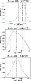 |
Fig. C.1 Comparison of NAMD values for the Kepler-462 system. The system consists of two planets on eccentric and misaligned orbits. Top: R-NAMD as defined in T20 using relative inclinations. Middle: λ-NAMD, using the projected spin–orbit angle (λ). Bottom: A-NAMD as defined in this work using the spin–orbit angle (ψ). The A-NAMD metric is the most suitable to capture the true architecture of the system. |
All Tables
All Figures
|
Fig. 1 R-NAMD versus multiplicity plot for the core sample described in the text; same as Fig. 3 in T20, but with an expanded sample. The horizontal offsets around the multiplicity values are added arbitrarily for better visualization. The color-scale, capped at one, represents the relative uncertainty on the R-NAMD values, obtained from the arithmetic mean of the lower and upper errors from the Monte Carlo method. Systems with relative uncertainty above unity are plotted with a hollow white circle. The linear fit is shown only as a visual aid as the slope is highly dependent on the (few) high-multiplicity systems. |
| In the text | |
|
Fig. 2 A-NAMD versus multiplicity plot. The systems shown are selected from the core sample on the basis of the availability of spin–orbit angle measurements, as described in the text. More systems are needed to confirm and quantify the sketched anticorrelation between A-NAMD and multiplicity. The linear fit is shown only as a visual aid. |
| In the text | |
|
Fig. 3 Comparison of NAMD values for the K2-290 system. The system consists of two planets on highly misaligned orbits. Left: R-NAMD as defined in T20 using relative inclinations. Middle: λ-NAMD, using the projected spin–orbit angle (λ). Right: A-NAMD as defined in this work using the spin–orbit angle (ψ). The A-NAMD is the most suitable to capture the true architecture of the system as it is not affected by projection effects. |
| In the text | |
|
Fig. 4 Four-quadrant diagram. This figure illustrates the possible states in which planetary systems can be found depending on their dynamical history, which is reflected in their eccentricities and spin–orbit angles. The Solar System is located at the intersection of the two gray dashed lines and separates the four quadrants, as discussed in the text. As an illustration, we include a value (red line) of a Solar System with planets misaligned by 15 degrees. The vertical highlighted area marks instead the R-NAMD values that can be associated with excited but stable systems that did not undergo large-scale instabilities in the simulations by Rickman et al. (2023). In addition, we included several synthetic systems based on real ones for which some parameters were missing (green points). These were inputted in order to better populate the quadrants. |
| In the text | |
|
Fig. C.1 Comparison of NAMD values for the Kepler-462 system. The system consists of two planets on eccentric and misaligned orbits. Top: R-NAMD as defined in T20 using relative inclinations. Middle: λ-NAMD, using the projected spin–orbit angle (λ). Bottom: A-NAMD as defined in this work using the spin–orbit angle (ψ). The A-NAMD metric is the most suitable to capture the true architecture of the system. |
| In the text | |
Current usage metrics show cumulative count of Article Views (full-text article views including HTML views, PDF and ePub downloads, according to the available data) and Abstracts Views on Vision4Press platform.
Data correspond to usage on the plateform after 2015. The current usage metrics is available 48-96 hours after online publication and is updated daily on week days.
Initial download of the metrics may take a while.