| Issue |
A&A
Volume 706, February 2026
|
|
|---|---|---|
| Article Number | A219 | |
| Number of page(s) | 15 | |
| Section | Numerical methods and codes | |
| DOI | https://doi.org/10.1051/0004-6361/202557334 | |
| Published online | 13 February 2026 | |
Dynamical evolution of massless particles in star clusters with NBODY6++GPU-MASSLESS
II. The long-term evolution of free-floating comets
1
Department of Physics, New York University Abu Dhabi,
PO Box 129188
Abu Dhabi,
UAE
2
Center for Astrophysics and Space Science (CASS), New York University Abu Dhabi,
PO Box 129188,
Abu Dhabi,
UAE
3
Astronomisches Rechen-Institut, Zentrum für Astronomie der Universität Heidelberg,
Mönchhofstrasse 12-14,
69120,
Heidelberg,
Germany
4
Dipartimento di Fisica, Sapienza, Universitá di Roma,
P.le Aldo Moro, 5,
00185
Rome,
Italy
5
Department of Physics, School of Mathematics and Physics, Xi’an Jiaotong-Liverpool University,
111 Ren’ai Road, Suzhou Dushu Lake Science and Education Innovation District, Suzhou Industrial Park,
Suzhou
215123,
PR China
6
Nicolaus Copernicus Astronomical Centre Polish Academy of Sciences,
ul. Bartycka 18,
00-716
Warsaw,
Poland
7
Szechenyi Istvan University, Space Technology and Space Law Research Center,
9026 Gyor, Egyetem ter 1.,
Hungary
8
Main Astronomical Observatory, National Academy of Sciences of Ukraine,
27 Akademika Zabolotnoho St,
03143
Kyiv,
Ukraine
9
National Astronomical Observatories and Key Laboratory of Computational Astrophysics, Chinese Academy of Sciences,
20A Datun Rd., Chaoyang District,
100101
Beijing,
China
10
Kavli Institute for Astronomy and Astrophysics, Peking University,
Yiheyuan Lu 5, Haidian Qu,
100871
Beijing,
China
★ Corresponding author: This email address is being protected from spambots. You need JavaScript enabled to view it.
Received:
20
September
2025
Accepted:
12
December
2025
Abstract
Context. Comets, asteroids, planetesimals, free-floating planets, and brown dwarfs are continuously injected into the intracluster environment after expulsion from their host-planetary systems or binary system. The dynamics of large populations of such free-floating comets (ffcs) in a star cluster environment is not yet fully understood.
Aims. We investigated the dynamical evolution of comet populations in star clusters and characterized the kinematics and ejection rates of ffc in a star cluster. Moreover, we determined whether a different initial energy distribution affects the mass segregation of the less massive population.
Methods. We carried out simulations using the N-body code NBODY6++GPU-MASSLESS, which allows the fast integration of star clusters that contain large numbers of massless particles, to characterize the dynamics of populations of low-mass particles with sub-virial and super-virial distributions.
Results. Comets do not participate in the mass-segregation process, similarly to planet-sized objects, regardless of their initial energy distribution. The latter slightly changed the whole dynamical evolution at the start of the simulation. We only observe an initial relaxation or collapse of the objects for super-virial and sub-virial ratios, respectively. The external regions of the ffcs population tend to be pulled back in the cluster core at the end of the simulation, suggesting the gravitational pull of the stars is pulling them back in the core. This phenomenon occurs at later times if the system is in virial equilibrium. Compared to less massive bodies, brown dwarfs experience more mass segregation. The inner regions tend to be more mixed with the stellar population.
Key words: methods: numerical / planets and satellites: dynamical evolution and stability / stars: kinematics and dynamics / open clusters and associations: general / galaxies: star clusters: general
© The Authors 2026
 Open Access article, published by EDP Sciences, under the terms of the Creative Commons Attribution License (https://creativecommons.org/licenses/by/4.0), which permits unrestricted use, distribution, and reproduction in any medium, provided the original work is properly cited.
This article is published in open access under the Subscribe to Open model. This email address is being protected from spambots. You need JavaScript enabled to view it. to support open access publication.
1 Introduction
Modern research into the dynamical evolution of comets began with Oort (1950). From the statistical properties of observed cometary orbits, Oort postulated the existence of a distant reservoir of comets with an inner radius of 50 000 au and an outer radius of 150 000 au as the origin of all the “new” long-time-period comets. This hypothetical cloud of comets is now known as the Oort cloud, and it is widely believed to be the source of the comets with orbital periods longer than 200 years. Several hundred comets have been identified in the recent centuries. These constitute only a tiny fraction of the comet reservoir in the Solar System. As comets in the Oort Cloud are not directly detectable, it is difficult to accurately estimate their abundance. A meticulous analysis of the kinematic properties of known long-period comets, as well as numerical simulations, can provide reasonable estimates of the present-day composition of the Oort Cloud (e.g., Oort 1950; Everhart 1967a,b; Weissman 1982, 1996; Wiegert & Tremaine 1999; Dones et al. 2004; Francis 2005; Fouchard et al. 2013; Shannon et al. 2015; Portegies Zwart 2021; Portegies Zwart et al. 2021; Bazyey & Bazyey 2022; Raymond et al. 2024, and references therein). Although results vary, these studies generally suggest that the number of comets brighter than H < 10.9 mag in the outer Oort cloud is on the order of 1011–1012. Numerical studies and extrapolations to smaller masses suggest that the present-day Oort cloud has a total mass of 2–40 Earth masses (see, e.g., Francis 2005; Morbidelli 2005).
During the epoch of planet formation, a large fraction of the planetesimals experienced gravitational scattering events that led to the ejection into the outer Solar System. The majority of these comets obtained velocities beyond the local escape velocity and became free-floating comets in the Galactic field, while others obtained highly eccentric orbits in the Oort cloud. Following the period of rapid ejection of comets, the Solar System entered a more quiescent phase, where comets are occasionally removed following a gravitational interaction with a planet or a neighboring star. It is estimated that over the course of ≈ 20 Myr close encounters with neighboring stars in the Galactic field – and the Galactic tidal force itself – have resulted into the dispersion of roughly 10% of the Oort Cloud into interstellar space (e.g., Biermann 1978; Weissman 1980; Dybczyński 2002; Torres et al. 2019).
Given the ubiquity of exoplanets in the Galactic field, it is not unreasonable to assume that a similar process also occurred during the early evolution of exoplanet systems and that the Milky Way is filled with comets and other free-floating debris. In fact, several studies claimed to have found evidence of so-called exocomets in systems such as β Pictoris (e.g., Welsh & Montgomery 2016, and references therein) and KIC 8462852 (e.g., Bodman & Quillen 2016; Boyajian et al. 2016, and references therein). The dynamical capture of these objects is rare (e.g., Valtonen & Innanen 1982; Torbett 1986). Occasionally, free-floating debris may interact with a planetary system, be captured, and possibly even collide with a star or planet.
Star clusters are potential candidates for hosting significant populations of free-floating planets and comets. The most recent discovery of candidate free-floating planets, made by Miret-Roig (2023) in the Scorpius association, includes thousands of planet-like objects and brown dwarfs. Free-floating planets have not yet been discovered in star clusters, although several candidates and a few confirmed free-floating planets have been found in associations (for a large microlensing survey; check Miret-Roig 2023). High-density environments, such as globular clusters, pose significant challenges to detecting planetary systems; this is even more significant for rare occurrences such as stellar occultation by free-floating planets. In nearby and less dense environments, such as open clusters, it is easier to detect such occurrences. However, they have not yet been found, as this would require a dedicated survey similar to the work of Miret-Roig (2023). Nevertheless, several studies Cai et al. (2019); Wu et al. (2023, 2024) with modeled debris disks hint at the existence of large, free-floating comet populations in star clusters. Their numerical simulations suggest that, among comet-like particles engulfed by flyby stars, a significant fraction of them will eventually reside inside their birth cluster. Moreover, the inclusion of disk-accompanying planets will further increase this fraction.
Close encounters between comet-hosting stars and other cluster members can result in the tidal stripping of comets from their host planetary systems. Both encounters and the tidal stripping from the comet-hosting star are responsible for the injection of debris into star clusters (e.g., Eggers et al. 1997; Dones et al. 2015; Brasser et al. 2008; Brasser 2008; Brasser & Schwamb 2015). As the velocity-at-infinity rate at which comets are ejected from their host planetary system is typically much lower than the local escape velocity, these comets remain part of the system and participate in the further dynamical evolution of the cluster until their escape from the cluster through ejection or evaporation (e.g., Wang et al. 2015). Such free-floating comets are captured by other stars (Kouwenhoven et al. 2010; Perets & Kouwenhoven 2012; Parker et al. 2017; Kokaia et al. 2022) and may be captured for longer times (e.g., Peñarrubia 2023), or even during the planet formation process (Pfalzner & Bannister 2019). The balance between a steady injection rate and escape of comets determines the total number of free-floating comets that is present in a star cluster at a given time. The number of free-floating substellar objects injected in the Galactic field is large. The number of free-floating planets (with Jupiter mass) is estimated to be 1/4th of the number of stars in the Galaxy (Mróz et al. 2018). Moreover, up to 1012 exo-comets are estimated to be present in the Galactic field for every star (Seligman & Moro-Martín 2022).
The ejection and capture of comets in star clusters occurs at a much higher rate than in the Galactic field. In these crowded stellar environments, many comets are expelled from their host stars due to the high frequency of close stellar encounters (e.g., Cai et al. 2019; Hands et al. 2019; Veras et al. 2020, and references therein). The following three processes are responsible for the presence of free-floating comets in star clusters: (i) the ejection of comets from their birth planetary systems due to interactions with (proto-)planets; (ii) ejections of comets from their planetary system following a close encounter with another star cluster member; and (iii) the escape of comets from their planetary system as their host star evolves and experiences phases of mass loss (see, e.g., Veras & Wyatt 2012).
Free-floating comets ejected from planetary systems in star clusters most likely have comparable speeds, and these ejection speeds are typically smaller than the local velocity dispersion in a star cluster (e.g., Spurzem et al. 2009; Zheng et al. 2015; Fujii & Hori 2019; Flammini Dotti et al. 2020; Wang et al. 2020, and references therein). Consequently, free-floating comets can remain bound to the star cluster for many dynamical times prior to their escape from the cluster (see Wang et al. 2015), during which the possibility for re-capture of a comet by another star arises.
Star-cluster members occasionally pair up and form new binary systems. Such newly formed systems are often transient (e.g., Moeckel & Clarke 2011), although some may survive for much longer times (e.g., Shu et al. 2020), in particular when they reside in the outskirts of the star cluster or when they are in the process of escaping from the star cluster (Kouwenhoven et al. 2010). Free-floating planets and free-floating planetary debris can also be captured (Perets & Kouwenhoven 2012; Parker & Quanz 2012; Zheng et al. 2015; Portegies Zwart 2021). Such captured bodies may be common (e.g., Siraj & Loeb 2021) and can be identified through their orbital parameter distributions (e.g., Siraj & Loeb 2019).
The process of mass segregation in different types of star clusters has been extensively and intensively studied (e.g., Fregeau et al. 2001; Allison et al. 2009; Olczak et al. 2011; De Vita et al. 2019; Adamo et al. 2020; Baumgardt et al. 2022). The process depends on the stellar-mass spectrum and is affected by both two-body relaxation and stellar evolution. However, studies on the impact of mass segregation on brown dwarfs are rare. It is important to highlight the study of Parker et al. (2016), which distinguishes the concept of mass segregation from the process of energy equipartition.
In this study, we considered the dynamical evolution of a population of free-floating comets (ffcs) in star clusters. We analyzed their kinematics using different energy distributions for the ffc population. Our findings are applicable to any population of bodies that can be approximated as massless, including comets, asteroids, planetesimals, and free-floating planets.
This paper is organized as follows. In Section 2, we briefly describe our numerical method and initial conditions. In Section 3, we discuss the dynamical evolution of the star clusters and the ffc populations. We also studied the ffc ejection rates. In Section 4, we try to theoretically predict whether the segregation of these small particles is possible or not. Finally, we summarize our results and discuss the implications of our findings in Section 5.
Initial conditions of the star-cluster models.
2 Methodology and initial conditions
We investigated the dynamical evolution of a population of ffcs in open clusters. We dynamically evolved three star-cluster models (C025, C05, and C075), each containing Ns=11 000 stars, and nffc=30 000 ffcs. Among the stars, nbin=1000 are in binary systems (according to the number of binaries expected from these systems; see, e.g., Offner et al. 2023, and references therein). We adopted the method of Sana et al. (2012) to pair the binaries. The semi-major axis of the binaries ranges from 0.01 to 100 au. Stellar masses were obtained from the Kroupa (2001a) initial mass function (IMF) in the 0.08−150 M⊙ mass range. The total mass of each star cluster is Mcl ≈ 6.62 × 10³ M⊙. The initial conditions of these models are listed in Table 1. We generated our model in a modified version of Mcluster (Küpper et al. 2011; Leveque et al. 2021), which generates free-floating comets along with the stellar population.
The positions and velocities for the stars were drawn from a Plummer (1911) model in virial equilibrium, with an initial virial radius of rvir=1.3 pc, corresponding to an initial half-mass radius of rhm=1.0 pc. The stars share the same density distribution in all models (i.e., they were generated with the same random seed). The positions of the ffcs were also drawn from a Plummer (1911) model using the same characteristics, except for the mass of the objects (and no IMF). We used a similar distribution, as we expected the ffcs to come from the protostellar phase of the stellar evolution and thus being a byproduct of stellar objects. Moreover, the velocities of the comets were scaled to obtain the desired virial ratio (Q=|T / U|, where T is the total kinetic energy and U is the total potential energy of the system) for our different models. Upon the generation of the ffc density distribution, all comets were assigned a mass. The kinetic energy was then changed according to the desired virial ratio of the ffcs population. As for the stellar generation, the kinetic energy was differently distributed, even though we used the same random seed. The ffcs in model C025 were assigned a sub-virial distribution (Q=0.25, where ffcs have, on average, lower velocities than the stellar distribution), those in model C050 were assigned virial equilibrium (Q=0.5), and those in model C075 were assigned a super-virial distribution (Q=0.75, where ffcs have, on average, higher speeds than the stellar distribution). We adopted these initial conditions to determine how the initial velocity distribution of ffcs affects their dynamical evolution over time and the mass segregation process. The stellar population is in virial equilibrium in all models.
Each star cluster evolves in an external tidal field corresponding to that of a Solar orbit in the Milky Way. The Milky Way is modeled as a point mass of MG=9.56 × 10¹⁰ M⊙, with the star cluster in a circular orbit with radius RG=8.5 kpc. The corresponding tidal radius (rt) of a cluster can then be estimated using rt ≈(Mcl / 3 MG)1 / 3 RG.
We used the method of NBODY6++GPU-MASSLESS1 (Flammini Dotti et al. 2025) to carry out our simulations. As the ffcs do not exert a gravitational force on the other bodies, they do not affect the evolution of the stellar population and the other ffcs. Stellar evolution and binary evolution were implemented following the prescriptions of the stellar-evolution package and their improvements (Eggleton et al. 1989; Hurley et al. 2000, 2002, 2005; Belczynski et al. 2007; Kamlah et al. 2022; Spurzem & Kamlah 2023).
We integrated the star-cluster models for 1000 Myr(≈ 25 trh.; see next section). Other important properties of the models, including the initial crossing time and initial half-mass relaxation time, are summarized in Table 1. The ffcs were treated as test particles during the simulations, unless noted otherwise.
3 Dynamical evolution of ffc populations
3.1 Timescales
The dynamical evolution of star clusters in this study remains predominantly influenced by the stars, as their mass is several orders of magnitude greater than that of the ffcs. Thus, the initial crossing time, tcr, and its initial half-mass relaxation time, trlx, depend on the stellar properties. The crossing time for the model (since we used the same stellar distribution in all the three models) is 0.25 Myr (see Table 1). The half-mass two-body relaxation time (Spitzer 1987) is defined as
 (1)
(1)
Here, rhm is the half-mass radius, ln Λ ≈ ln (0.02 Ns) is the Coulomb logarithm for different population masses (Giersz & Spurzem 1994), and Ns is the number of stars. In physical units, the initial half-mass relaxation time is 40.63 Myr. The mass-segregation timescale in the generic model is tms= trlx mav / mmax ≈ 0.006 trlx ≈ 0.24 Myr. For reference, the disruption timescale of the star cluster (Lamers et al. 2005) is approximately 6.6 Gyr. In the following sections, we analyze an alternative approach to the mass-segregation timescale, which we used in this work to analyze the long-term dynamics of the smaller sized objects and to confirm whether, with N-body direct simulations, it is indeed possible to observe mass segregation of these low-mass objects.
3.2 Lagrangian radii
Lagrangian radii provide a powerful tool for analyzing the global evolution of a star cluster. The evolution of the Lagrangian radii for all simulated models is depicted in Figures 1, 2, and 3. For the peaks in the ffcs Lagrangian radii, they are due to an ffc particle that is on the verge of escaping the cluster. For a more detailed explanation, please see the previous paper of this series (Flammini Dotti et al. 2025). At each moment in time, the Lagrangian radii for the stars are calculated relatively to the total cluster mass at that time. The Lagrangian radii for the massless particles depend solely on the number of ffcs within the Lagrangian shell at the actual time, as all ffcs have the same mass.
Over time, the star cluster undergoes gradual expansion and mass loss, driven by stellar evolution and the escape of stars from the cluster. It is important to note that the stellar Lagrangian radii, as shown in Figures 1 and 2, are independent of the properties of the ffc population. Since ffcs are massless, their presence does not influence the dynamical evolution of the stellar population.
For the stellar population, at t ≈ 8 Myr, the cluster core undergoes a slight contraction, followed by a rebound. This event triggers strong scattering, resulting in the ejection of stars to the outskirts of the star cluster and beyond. Simultaneously, stellar evolution contributes to a gradual reduction in the cluster’s total mass. Over the course of approximately 20 Myr, these processes lead to the loss of about 10% of the cluster’s initial total mass. As a result of stellar ejections and stellar mass loss, the gravitational potential of the star cluster decreases.
The dynamical evolution of the ffc population is linked to the evolution of the core of the star cluster (Flammini Dotti et al. 2025). In the inner regions of all models, the ffcs exhibit a similar orbital behavior around the core (Figure 1). During the first ∼ 0.5 Myr, the innermost regions of the ffc population undergo contraction and expansion in models C025 and C075, respectively. This is driven by the contraction due to the low average velocity of the ffcs and the escape of high-velocity ffcs in models C025 and C075, respectively. The 50% shells of the ffcs population behave similarly in all models after ∼ 1 Myr. After this initial phase of contraction and expansion in the two different models, the inner regions behave mostly similarly for all models. In the 0.1% shell, the ffcs tend to orbit the core at a larger distance than the stars. We also have a similar evolution for the 50% shell, which is slowly expanding compared to the stellar 50% shell.
In the outer regions (Figure 2), the behavior is similar for all three models, but we experience a retraction in both C025 and C075 models. Since ffcs have already lost more than 50% of the particles and possibly the highest energy members have been ejected, the 90% shell of ffc is contracting rather than expanding. However, this shell clearly tends to shrink around 800 Myr in models C025 and C075, while the model C050 (initially in virial equilibrium) also begins to contract, although less noticeably (extending the simulations by another 20 Myr confirms a similar trend). This behavior arises from the gradual loss of kinetic energy among the ffcs and the occurrence of ejections. Since model C075 experiences slightly more ejections (see Section 3.4), the outer ffcs are more strongly affected by the gravitational potential of the core and move inward. Similarly, in model C025, the total kinetic energy of ffcs is lower than in the other two models, so they are more efficiently pulled toward the center. At this stage, the average velocity of the ffcs is low enough that they become influenced by the deeper potential well of the core, causing them to move inward and remain confined in the inner regions.
The velocity dispersion shown in Figure 4 confirms our previous conclusions. The stellar population has a larger velocity dispersion compared to that of the ffc population, and the velocity dispersion of the ffcs gradually reduces in all models. The initial imprint of the different velocity distribution is clearly present in models C025 and C075, but it rapidly vanishes within less than 1 Myr. The results also imply that ffcs do not follow mass segregation.
One may wonder whether the ffcs would participate in the energy equipartition, since there is a large difference in energy between the population, or similar energy, respectively in the C025 and C075 models. The mass difference between the components in a star cluster is significant when also considering planets or comets. If we only include stars (e.g., 0.08 M⊙ to ≈ 60 M⊙), the mass ratio is roughly two orders of magnitude. Compared to the average mass (≈ 0.58 M⊙), the mass ratio is typically one order of magnitude. Planets and comets, on the other hand, are much less massive than stars. Such bodies are dynamically irrelevant to the evolution of the star cluster. Moreover, with the global dynamical evolution of ffcs, we show that this phenomenon is not energy dependent, as all three models have a relatively similar behavior after just several Myr.
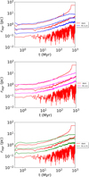 |
Fig. 1 Evolution of Lagrangian radii enclosing 0.1%, 10%, and 50% of the total mass for stars and percentage of ffcs (indicated in the legend with the virial ratio of the model), for the models C025 (top), C05 (middle), and C075 (bottom). At each time step, the Lagrangian radii were calculated based on the total mass of the star cluster at that time. |
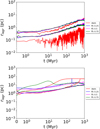 |
Fig. 3 Top: evolution of Lagrangian radii containing mass of 0.1% and 10% for both stars and percentage of ffcs from each model. Bottom: same, but for 50% and 90% Lagrangian radii. The Lagrangian radii at each time were calculated using the total mass of the star cluster at that time. |
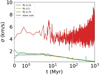 |
Fig. 4 Velocity dispersion of stellar population and ffc population. The ffc velocity dispersion is smaller than that of the stellar population in all models. The presented velocity dispersion considers the center of mass for the binary systems. A zoomed-in view of the ffcs’ curves is in Appendix E. |
3.3 Kinematical evolution of ffcs in star clusters
We simulated models in which the ffcs have different initial velocities; therefore, the distribution resulting for equal-mass ffcs depends mainly on their speeds. The speeds differ between the three models, as shown in Figure 5. The square velocity of these systems at the start of the simulation (top panel) is quite different, with speed ranging between the maximum velocity of model C075 (≈ 13.36 km s−1) and the minimum speed of model C 025(≈ 0.03 km s−1). The average initial speeds are 1.91, 3.31, and 5.73 km s−1 for model C025, C05, and C075, respectively. After 1000 Myr (bottom panel), the ffc distributions of all models are similar. The same plot, with separated ffc for all models, is present in Appendix C. The minimum speed of models ranges from 2.79 × 10⁻² km s−1 for model C025 to a maximum of 5.19 km s−1 for model C025. The average values are 0.76, 0.76, and 0.85 km s−1 for models C025, C05, and C075, respectively. Appendix C shows the distributions for each model.
Three key conclusions can be drawn from comparing the ffc distributions at the start and at the end of the simulations: (i) the distribution of particles is quite similar for all models at the end of the simulation, which tells us that the imprint of the initial conditions disappeared; (ii) the position of the remaining particles is mostly moving in the inner orbits, while the outer regions have barely changed, testifying that the core is pulling the ffcs in – the mass of the core remains quite similar for all the models (see Appendix B; the radius and mass of the core in the star cluster for model C05); and (iii) the high-velocity ffcs have escaped from the cluster, leaving those with speeds below roughly 1 km s−1. The latter observation is especially important, as we can assume that any ffcs with sufficient initial speed to escape from the inner regions of the cluster ultimately did so. For our initial conditions, the escape velocity from the cluster center at t=0 Myr is vesc=3.31 km s−1. Thus, close encounters with stars will eventually result in the ejection of objects at higher velocities within just several million years. Subsequently, other ffcs are ejected either from tidal stripping in the outer regions or evaporation.
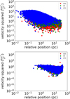 |
Fig. 5 Radial positions and square velocities of ffcs, for all simulated models, at t=0 Myr (top panel) and at the end of the simulation at t= 1000 Myr (bottom panel). We also added every single model separately from the rest in Appendix D. |
3.4 Escaping stars and ffcs
Figure 6 shows the cumulative fraction of ejected particles. The stellar ejection rates are identical for all three models. The total number of ejected stars at t=1000 Myr is 4736(47.36% of the initial number of stars), while the total number of ejected ffcs is 18355, 17625 and 18367, respectively, for models C025, C05, and C075 (corresponding to 61.18%, 58.75%, and 61.22% of the initial total number of ffcs). The higher number of ejected particles is due to the relatively low density of the star cluster in the initial conditions. Moreover, we can see that the total number of ejected ffcs is similar in all models, further justifying their independence from their initial conditions. At the start of the simulation we can clearly see a major difference in ejection due to the energy distribution of the ffcs, where the C075 model ejects 25% of particles over a few million years and then proceeds almost linearly until the end of the simulation. Model C025, instead, evolves as a logarithmic curve up until 300 Myr and then proceeds linearly. The model in virial equilibrium, C05, behaves similarly to the stellar cumulative curve, with an initial difference due to stellar evolution. Thus, we can conclude that the imprint of initial conditions is mainly observed at the start of the simulation, on a timescale shorter than a relaxation time.
Consistently with previous studies and with Flammini Dotti et al. (2025), the ejection speeds of stars and ffcs display the same larger velocities for stars and smaller ones for ffcs during the ejection. As observed in earlier work of this series, the stars with the highest speeds are neutron stars (see Appendix D).
The average velocities of the ejected stellar population are 10.02 km s−1 for all models, while the corresponding values for the ejected ffcs are 1.22 km s−1, 1.29 km s−1, and 1.91 km s−1 for models C025, C05, and C075, respectively. The slight difference in average speed is due to the initial ejection of ffcs, which is slightly faster in model C075 and slightly slower in models C025 and C05. This is a consequence of the diverse initial energy distribution, which gave larger velocities in model C075 and smaller velocities in model C025. Except for random fluctuations in the ejection velocities, we have the same velocity distribution in the ejected particles.
In the following section, we present an alternative approach to the mass-segregation timescale, which we used in our study of the long-term dynamics of the lower-mass objects and to determine with N-body simulations whether such populations indeed experience mass segregation.
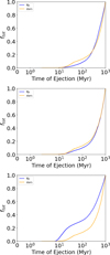 |
Fig. 6 Cumulative ejection distribution of escapers, including both stars and ffcs. Notably, the ejection function for all three ffc models shows variation only at the beginning, after which it progresses almost linearly. |
4 Mass segregation with two different populations
4.1 Relaxation and mass-segregation times for LMP
We saw that the ffcs, in a long-term dynamical-evolution scenario, are either ejected through evaporation or ejection at high velocities, mostly due to the type of models we chose. In this section, we describe a more general approach, using the initial conditions of our previous models as an example, but not using the simulation data. The role of segregation of low-mass particles (such as comets) in a star cluster is an interesting topic. These particles do not follow mass segregation (as that shown in the previous paper of this series; see Flammini Dotti et al. 2025, and here). Thus, these particles should not segregate independently and should be mostly governed by the inner regions, despite the number of particles and their mass.
Following Appendix A, we considered low-mass particles as anything that is not considered a star. We therefore assumed a maximum mass of 0.08 M⊙ (brown dwarfs) and a minimum mass of the comets for the low-mass particles. We used the same terms, LMP and HMP, since we effectively describe several types of objects for LMP. We used these terms until the end of Section 4.
For all purposes, we used Equation (3.1) for the “classical” relaxation time. We used the following expressions for the masssegregation timescale:
 (2)
(2)
 (3)
(3)
which are the coupled and uncoupled mass-segregation timescales, respectively. The derivation and interpretation of these expressions are provided in Appendix A.
Figure 7 shows the evolution of the relaxation timescale in terms of the decoupled relaxation time, using the initial conditions of our reference models, excluding the LMP mass. For the LMP, using the same initial conditions of this work, we find that trlx, LMP ≈ 3.46 × 10⁸ Myr, which is four orders of magnitude larger than the Hubble time.
A similar conclusion is found for terrestrial-like planets. Interestingly, using a mass spectra of an LMP population ranging from 1 ME to 1 MJ in a logarithmic uniform distribution, the timescale for relaxation is quite low for these masses.
Finally, for our model, we see that the LMP have an acceptable timescale (on the order of a gigayear) for masses near the stellar limit. This approximation of the relaxation timescale is only valid for low masses, as otherwise the stellar population would not decouple from the LMP.
The previous results give us two important conclusions: (i) the mass spectra for a planetary population, as shown in the figure, may effectively be significant when we want to define how the LMP evolves dynamically; and (ii) near-stellar masses, such as brown dwarfs, are likely to follow mass segregation on comparable timescales to those of stellar populations. The former point is interesting in its own “internal segregation”, in which we may check how the Earth-sized planets evolve as compared to the Jupiter-like planets.
We therefore wish to determine the threshold mass of an LMP not to be decoupled from the stellar population. We analyze this limit in terms of its mass-segregation timescale in the next section. We consider the relaxation time of the decoupled population, but we have also taken into account the average stellar mass of the cluster used in our model. If we consider the decoupled mass-segregation timescale, the term mav / mmax, with same-mass LMP, is unity.
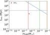 |
Fig. 7 Relaxation timescale of LMP population for different masses using our initial conditions for the number of LMP and the half-mass radius. The relaxation timescale for an Earth mass and a Jupiter mass are from the red line and green line, respectively. The orange line shows the star limit (i.e., the ignition of hydrogen at ≈ 0.08 M⊙). The red dot shows the timescale considering a mass spectra of LMP in a uniform logarithmic distribution, ranging from Earth mass to Jupiter mass, using the same initial condition of our main models. Finally, the blue line shows results taking into account the initial conditions of the model C05. |
4.2 Analysis of the decoupled mass-segregation timescale
From the timescales we discussed in Appendix A, we can effectively compare and analyze the mass-threshold value for the particles to be included in the mass segregation process. There is a strong dependence, in the LMP, on the number of their objects and their mass. Smaller Nffc and larger mffc would result in a smaller timescale. Although not analyzed in this work, the (initial) spatial and velocity distribution of the LMP is also rather important, especially if the LMPs are formed in an overall smaller region of the cluster.
Our results are similar to those for same-mass clusters, where mass segregation is a greater cause of same-mass elements. However, compared to that case, there is no stellar evolution for the LMP.
In Figure 8, we show the mass-segregation timescale as a function of the mass of the LMP and the number of LMPs, respectively, in the left and right plots, assuming the star cluster initial condition used in this work. We can immediately tell that the coupled-mass-segregation term does not bring result according to any result obtained to date in the literature, and that the mass-segregation timescale does not agree with our simulations (and it partly disagrees with brown dwarfs, as we see in the next section). The decoupled mass segregation seems to be more in agreement with our results on the relaxation timescale. To obtain a broader understanding of the possible scenario, we list the result observed for the different LMP used in Figure 8:
If we use comet-mass objects, their mass can be any dimension smaller than a planetary mass. A mass average value would be 10−14 M⊙, while we constructed more massive comets, on the order of 10−11 M⊙, for this simulation. Within our initial conditions, the mass-segregation-coupled timescale is too large (tms, LMP=4.61 × 10⁸ Myr). The same is true for a larger number of LMPs, as the number grows exponentially (linearly on a log scale).
If we use planet-mass objects, we have tms, LMP=1.46 × 10³ Myr and 4.61 × 10⁴ Myr for a Jupiter-like mass and Earth-like mass, respectively. Earth-like objects shares the same issue as comets, with a timescale longer than a Hubble time. The Jupiter-mass planets seems the most suitable candidates for our initial conditions, instead.
For brown dwarfs, the mass-segregation timescale is tms, LMP=1.63 × 10² Myr, and thus it is the more accurate candidate to test the mass-segregation limit (see next section).
The case of mass spectra is particularly interesting and worth testing. Whether the masses are gravitationally pulled by the inner regions similarly to other cases or whether they manage to relax before this occurs is the main idea for the next work.
In the previous list of results we opted not to include the HMP mass-segregation timescale, but this is indeed an important factor. Since these populations will segregate faster, we expect the cluster to have evolved at a significant distance with regard to its initial conditions after the cluster relaxed. This may be especially useful in low-density star clusters. We will consider this in future works. Thus, the LMP with masses significantly smaller than those of stars become decoupled and exhibit very long mass segregation timescales. In our previous assumptions, we left the half-mass radius at a similar value in both cases. A more concentrated distribution in the center or a more enlarged distribution, as seen in Sections 3.2 and 3.3, would just remove particles in the outermost regions, while objects would continue to orbit in the cluster center. The assumption of similar initial conditions between ffcs and stars makes more sense than a completely diverse one, as comets are a byproduct of stellar and proto-planetary disks. The initial energy, as shown in the previous section, does not diverge too far from the final results. Thus, a final confirmation is needed in terms of a mass spectrum for the planets.
We also carried out a simulation using brown dwarfs instead of comets, as we show in the next section. We plan to analyze the upper limits of “non-stellar” objects to observe the dynamical behavior of the latter for near-stellar mass objects.
4.3 Dynamical evolution of brown dwarfs and asymptotic mass segregation
With the results coming from a simulation of brown dwarfs, using the initial conditions of Table 1 but the mass of the ffcs gives extremely interesting results. For a more direct comparison of what was argued in the previous section, we show the dynamical evolution of brown dwarfs in Figure 9, using the same set of initial conditions of Table 1, except for the mass of the “massless objects.” We used the classic version of NBODY6++GPU for this simulation. We did so because brown dwarfs are extremely close to the stellar mass, and thus the massless approximation we previously applied is no longer eligible.
The number of ejected stars and brown dwarfs is lower than the stellar and ffc counterpart, as the model is much more massive overall. 14.48% of stars are ejected, and 16.18% of brown dwarfs are ejected at the end of the simulation.
We observe a similar evolution of the Lagrangian radii compared to that of the comets. However, there are also several differences: (i) at around 80 Myr, we see a peak in the outer regions, which suggests a partial mass segregation of these objects (as suggested in the bottom plot of Figure 9); and (ii) the populations in the inner regions are more mixed, and the bump in average mass around 200 Myr is in line with the mass-segregation-decoupled timescale. It is quite interesting to see that there is indeed a second inverse segregation that is a direct consequence of the mixing between the two populations. This is due to the total mass of the brown dwarfs being comparable with the core mass. In this specific case, it is also slightly larger by a factor of 100 M⊙. Since the masses are comparable, there is a slight mixing, with some brown dwarfs orbiting the core, and some segregating in the outer regions. Although not extremely precise, the brown dwarfs are indeed the mass limit for an object to effectively segregate in a cluster. A different set of initial conditions (e.g., a larger number of brown dwarfs) would make this difference more significant.
Thus, our previous approach to the mass-segregation timescale is only partly correct, as it does not take into account the mass difference in the populations, though these are treated as decoupled. This is related to the thermodynamical behavior of the system.
We now reconsider a general approach using HMP and LMP for the cluster populations. According to Gomez-Leyton & Velazquez (2019), concerning the mass segregation of a multi-populated mass system such as ours, the mass segregation of the smallest component does not behave in the classical way, but asymptotically. If the mcore, HMP ≫ NLMP mLMP, where mcore is the core mass of the HMP, then the secondary population should not segregate. Thus, mass segregation effectively occurs when the total mass of the LMPs is closer to that of the inner regions. We therefore expect the system to not segregate even a larger masses. This conclusion affects the astrophysical implications of this study, and it justifies the results shown in Section 3. Thus, the core mass is the effective thermodynamical catalyst for the evolution of our LMP. This cannot happen for planetsized objects, and it would only happen for near-stellar-sized components (similar to multiple stellar populations in globular clusters). Hence, both observed open clusters and globular clusters are not ideal candidates for mass-segregated populations for the following reasons:
Open clusters are less dense, but have extremely short timescales for cluster dissolution. A near-dissolution star-cluster candidate may be the best case to observe whatever the LMP segregated in that case.
Globular clusters have extremely long dissolution timescales, and thus the cluster would remain much more massive than the LMP population.
Specific cases, such as substructured clusters or tidal tails, would be interesting prospects to observe this population as segregated, at least locally.
The only remaining factor to understand is whether a mass spectrum of planets is a redundant idea or not. The same work of Gomez-Leyton & Velazquez (2019) showed a dependence on both the total mass and the single mass of the components of the two populations. Thus, more unequal populations may lead this study in another direction and prove if both these systems are decoupled and are only dependent on the core mass, even with a different mass distribution. An internal segregation of only the planet-sized particles could highlight a different aspect with regard to this topic. We will focus on the latter in the next work of this series.
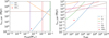 |
Fig. 8 Mass segregation timescale of LMP population for different masses (left) and number of initial objects (right) using our initial conditions for the number of LMP and the half-mass radius. In the left plot, we show the mass segregation timescale for coupled (MSTc) and decoupled (MSTdc) timescales. MSPEJ is instead the mass segregation timescale for a decoupled mass spectrum from Earth to Jupiter masses, distributed in a logarithmic uniform distribution. On the right, with similar semantics, we have Earth, Jupiter, and a brown dwarf coupled (c suffix) and decoupled (dc suffix). The relaxation timescale for a Jupiter mass and an Earth mass are indicated with the orange and green lines, respectively. |
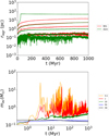 |
Fig. 9 Top: Lagrangian radii evolution of both stellar and brown-dwarf components in the 0.1%, 1%, 10%, 50%, and 90% shells. The Lagrangian radii evolution is green for the stellar components and red for the brown dwarfs. Bottom: with identical shells, we display the average mass evolution. |
5 Conclusions
In the first paper of this series (Flammini Dotti et al. 2025), we explored the dynamical evolution of massless particles. We concluded that, even with varying cluster densities, the dynamical evolution is primarily determined by the core’s evolution rather than being influenced by mass segregation. In this second work, we instead modified the energy distribution of the massless particles, which, on a technical level, corresponds to varying their kinetic energies. Moreover, we analyzed the kinematics of ffcs and their escape rates. Finally, we show the mass-segregation limits for massless particles as compared to the respective stellar component, highlighting the thermodynamical aspect of the system, resulting in the HMP core being the main catalyst for the mass segregation of the LMP. Given our conclusion, there are only extremely specific cases in which we could observe segregation of free-floating comets or planets. The main results of our study can be summarized as follows:
The spatial distributions and kinematics of the three models of the ffc population diverges at the start for the non-virialized models, which virialize shortly after. This effect is quite fast, that is, on the order of 0.5 Myr, which is ≈ 2 tms. This process is mainly related to the high-velocity ffcs being ejected in model C075 and to the stellar encountering other stars in the model C025. These events substantially change the overall kinetic energy of the particles. The system becomes virialized on a short timescale, which means that mass segregation is not achieved in faster (or shorter) times for different energies;
Interestingly, the 90% Lagrangian shell of models C025 and C075 causes both stars to contract around 25 relaxation times. The C05 model also contracts some megayears later. This is related to the particles being attracted to the core, when high energy ffcs are ejected and a large number of the ffcs are evaporated, leaving just low-velocity objects. Moreover, the ffc population drastically dropped to ≈ 40%, resulting in a less populated, and thus less diversified, ffc population, which lost any imprint of the initial energy distribution;
Brown dwarfs follow a different path to comets, as their results hint at a more mixed dynamical behavior for these objects orbiting the core similarly to the ffcs, and they are also mixed in the innermost regions as stellar components. An interesting result is an inverse mass segregation at around 200 Myr, where most brown dwarfs are mixed in the innermost regions;
The study on the mass segregation of massless particles follows and confirms the conclusions of Gomez-Leyton & Velazquez (2019) and proves that the stellar mass in the star-cluster core is fundamental for the evolution of the massless particles. The system relaxes violently at the start for non-virialized systems, but this is mostly related to the initial conditions (i.e., velocities) of the ffcs;
Spatial separation (“mass segregation”) of ffcs is highly unlikely in open clusters (which dissolve quite rapidly), but interesting to check in dissolution-like scenarios. Globular clusters (which dissolve too slowly and have core masses significantly higher than the population of ffcs) represent an improbable scenario.
We did not include any planetary companions among star cluster members. Realistic planetary systems may alter the orbits of captured ffcs through gravitational interaction during periastron passage. Although integrating multi-planet systems in a comparatively short time is still challenging in N-body direct simulation, substantial progress has been made over since 2007 (e.g., Malmberg et al. 2007; Hao et al. 2013; Shara et al. 2016), and combining simulations of star clusters with those of planetary systems is now possible using the AMUSE software environment (see Portegies Zwart et al. 2013; Pelupessy et al. 2013; Cai et al. 2016) by sequentially integrating the stellar and planetary components (e.g., Cai et al. 2015, 2017; Flammini Dotti et al. 2018, 2019, 2020; Stock et al. 2020; Flammini Dotti et al. 2023; Wu et al. 2023, 2024). This is a necessary step for obtaining a full understanding of ffc populations in star clusters, and in particular for understanding the transfer of material between planetary systems through physical collisions between planets and exo-comets.
Finally, large numerical simulations with a high number of ffcs would solve this paradigm definitively. However, we still lack adequate direct N-body codes (or super-computing resources) to reach the minimum possible (≈ 108 ffcs) in order to obtain a plausible number of ffcs for these simulations.
Acknowledgements
We thank the anonymous referee for the comments, which helped to improve dramatically the quality of our work. This material is based upon work supported by Tamkeen under the NYU Abu Dhabi Research Institute grant CASS. FFD, RS, and KW acknowledge support by the German Science Foundation (DFG, project Sp 345/24-1). A.A. acknowledges support for this paper from project No. 2021/43/P/ST9/03167 co-funded by the Polish National Science Center (NCN) and the European Union Framework Programme for Research and Innovation Horizon 2020 under the Marie Skłodowska-Curie grant agreement No. 945339. This research was funded in part by NCN grant number 2024/55/D/ST9/02585. P.B. thanks the support from the special program of the Polish Academy of Sciences and the U.S. National Academy of Sciences under the Long-term program to support Ukrainian research teams grant No. PAN.BFB.S.BWZ.329.022.2023. M.G. was supported by the Polish National Science Center (NCN) through the grant 2021/41/B/ST9/01191. K.W. and R.S. acknowledge support by German Science Foundation (DFG) under grant Sp 345/24-1. K.W. and R.S. acknowledges NAOC International Cooperation Office for its support in 2023, 2024, and 2025, and the support by the National Science Foundation of China (NSFC) under grant No. 12473017. This research was supported in part by grant NSF PHY-2309135 to the Kavli Institute for Theoretical Physics (KITP). K.W. acknowledge SPP 1992, a Priority Program funded by the Deutsche Forschungsgemeinschaft (DFG), for the support during the visit to Heidelberg, Germany in March and April 2024.
References
- Adamo, A., Kruijssen, J. M. D., Bastian, N., et al. 2020, Space Sci. Rev., 216, 51 [Google Scholar]
- Allison, R. J., Goodwin, S. P., Parker, R. J., et al. 2009, MNRAS, 395, 1449 [Google Scholar]
- Baumgardt, H., et al. 2022, MNRAS, 510, 3531 [Google Scholar]
- Bazyey, O., & Bazyey, N., 2022, Astron. Astrophys. Trans., 33, 5 [Google Scholar]
- Belczynski, K., Taam, R. E., Kalogera, V., Rasio, F. A., & Bulik, T., 2007, ApJ, 662, 504 [Google Scholar]
- Biermann, L., 1978, in Astronomical Papers Dedicated to Bengt Stromgren, eds. A. Reiz, & T. Andersen, 327 [Google Scholar]
- Bodman, E. H. L., & Quillen, A., 2016, ApJ, 819, L34 [NASA ADS] [CrossRef] [Google Scholar]
- Boyajian, T. S., LaCourse, D. M., Rappaport, S. A., et al. 2016, MNRAS, 457, 3988 [NASA ADS] [CrossRef] [Google Scholar]
- Brasser, R., 2008, A&A, 492, 251 [NASA ADS] [CrossRef] [EDP Sciences] [Google Scholar]
- Brasser, R., & Schwamb, M. E., 2015, MNRAS, 446, 3788 [Google Scholar]
- Brasser, R., Duncan, M. J., & Levison, H. F., 2008, Icarus, 196, 274 [Google Scholar]
- Cai, M. X., Meiron, Y., Kouwenhoven, M. B. N., Assmann, P., & Spurzem, R., 2015, ApJS, 219, 31 [Google Scholar]
- Cai, M. X., Spurzem, R., & Kouwenhoven, M. B. N., 2016, in IAU Symposium, Star Clusters and Black Holes in Galaxies across Cosmic Time, eds. Y. Meiron, S. Li, F.-K. Liu, & R. Spurzem, 312, 235 [Google Scholar]
- Cai, M. X., Kouwenhoven, M. B. N., Portegies Zwart, S. F., & Spurzem, R., 2017, MNRAS, 470, 4337 [Google Scholar]
- Cai, M. X., Portegies Zwart, S., Kouwenhoven, M. B. N., & Spurzem, R., 2019, MNRAS, 489, 4311 [NASA ADS] [CrossRef] [Google Scholar]
- De Vita, A., et al. 2019, MNRAS, 485, 5752 [Google Scholar]
- Dones, L., Brasser, R., Kaib, N., & Rickman, H., 2015, Space Sci. Rev., 197, 191 [NASA ADS] [CrossRef] [Google Scholar]
- Dones, L., Weissman, P. R., Levison, H. F., & Duncan, M. J., 2004, in Astronomical Society of the Pacific Conference Series, Star Formation in the Interstellar Medium: In Honor of David Hollenbach, eds. D. Johnstone, F. C. Adams, D. N. C. Lin, D. A. Neufeeld, & E. C. Ostriker, 323, 371 [Google Scholar]
- Dybczyński, P. A., 2002, A&A, 396, 283 [NASA ADS] [CrossRef] [EDP Sciences] [Google Scholar]
- Eggers, S., Keller, H. U., Kroupa, P., & Markiewicz, W. J., 1997, Planet. Space Sci., 45, 1099 [Google Scholar]
- Eggleton, P. P., Fitchett, M. J., & Tout, C. A., 1989, ApJ, 347, 998 [NASA ADS] [CrossRef] [Google Scholar]
- Everhart, E., 1967a, AJ, 72, 716 [Google Scholar]
- Everhart, E., 1967b, AJ, 72, 1002 [Google Scholar]
- Flammini Dotti, F., Cai, M. X., Spurzem, R., & Kouwenhoven, M., 2018, Proc. Int. Astron. Union, 14, 293 [Google Scholar]
- Flammini Dotti, F., Kouwenhoven, M. B. N., Cai, M. X., & Spurzem, R., 2019, MNRAS, 489, 2280 [NASA ADS] [CrossRef] [Google Scholar]
- Flammini Dotti, F., Kouwenhoven, M. B. N., Shu, Q., Hao, W., & Spurzem, R., 2020, MNRAS, 497, 3623 [Google Scholar]
- Flammini Dotti, F., Capuzzo-Dolcetta, R., & Kouwenhoven, M. B. N., 2023, MNRAS, 526, 1987 [NASA ADS] [CrossRef] [Google Scholar]
- Flammini Dotti, F., Kouwenhoven, M. B. N., Berczik, P., Shu, Q., & Spurzem, R., 2025, A&A, 693, A166 [NASA ADS] [CrossRef] [EDP Sciences] [Google Scholar]
- Fouchard, M., Rickman, H., Froeschlé, C., & Valsecchi, G. B., 2013, Icarus, 222, 20 [Google Scholar]
- Francis, P. J., 2005, ApJ, 635, 1348 [NASA ADS] [CrossRef] [Google Scholar]
- Fregeau, J. M., Joshi, K. J., Portegies Zwart, S. F., & Rasio, F. A., 2001, AJ, 562, L5 [Google Scholar]
- Fujii, M. S., & Hori, Y., 2019, A&A, 624, A110 [NASA ADS] [CrossRef] [EDP Sciences] [Google Scholar]
- Giersz, M., & Spurzem, R., 1994, MNRAS, 269, 241 [Google Scholar]
- Gomez-Leyton, Y. J., & Velazquez, L., 2019, MNRAS, 488, 362 [Google Scholar]
- Hands, T. O., Dehnen, W., Gration, A., Stadel, J., & Moore, B., 2019, MNRAS, 490, 21 [Google Scholar]
- Hao, W., Kouwenhoven, M. B. N., & Spurzem, R., 2013, MNRAS, 433, 867 [Google Scholar]
- Hurley, J. R., Pols, O. R., & Tout, C. A., 2000, MNRAS, 315, 543 [Google Scholar]
- Hurley, J. R., Tout, C. A., & Pols, O. R., 2002, MNRAS, 329, 897 [Google Scholar]
- Hurley, J. R., Pols, O. R., Aarseth, S. J., & Tout, C. A., 2005, MNRAS, 363, 293 [NASA ADS] [CrossRef] [Google Scholar]
- Kamlah, A., Leveque, A., Spurzem, R., et al. 2022, MNRAS, 511, 4060 [NASA ADS] [CrossRef] [Google Scholar]
- Kokaia, G., Davies, M. B., & Mustill, A. J., 2022, MNRAS, 511, 1685 [Google Scholar]
- Kouwenhoven, M. B. N., Goodwin, S. P., Parker, R. J., et al. 2010, MNRAS, 404, 1835 [NASA ADS] [Google Scholar]
- Kroupa, P., 2001a, MNRAS, 322, 231 [NASA ADS] [CrossRef] [Google Scholar]
- Kroupa, P. 2001b, in Astronomical Society of the Pacific Conference Series, 228, Dynamics of Star Clusters and the Milky Way, eds. S. Deiters, B. Fuchs, A. Just, R. Spurzem, & R. Wielen, 187 [Google Scholar]
- Küpper, A. H., Maschberger, T., Kroupa, P., & Baumgardt, H., 2011, MNRAS, 417, 2300 [CrossRef] [Google Scholar]
- Lamers, H. J. G. L. M., Gieles, M., Bastian, N., et al. 2005, A&A, 441, 117 [NASA ADS] [CrossRef] [EDP Sciences] [Google Scholar]
- Leveque, A., Giersz, M., & Paolillo, M., 2021, MNRAS, 501, 5212 [NASA ADS] [CrossRef] [Google Scholar]
- Malmberg, D., de Angeli, F., Davies, M. B., et al. 2007, MNRAS, 378, 1207 [NASA ADS] [CrossRef] [Google Scholar]
- Miret-Roig, N., 2023, Ap&SS, 368, 17 [NASA ADS] [CrossRef] [Google Scholar]
- Moeckel, N., & Clarke, C. J., 2011, MNRAS, 415, 1179 [NASA ADS] [CrossRef] [Google Scholar]
- Morbidelli, A., 2005, arXiv e-prints [arXiv:astro-ph/0512256] [Google Scholar]
- Mróz, P., Ryu, Y.-H., Skowron, J., et al. 2018, AJ, 155, 121 [Google Scholar]
- Offner, S. S. R., Moe, M., Kratter, K. M., et al. 2023, in Astronomical Society of the Pacific Conference Series, Protostars and Planets VII, eds. S. Inutsuka, Y. Aikawa, T. Muto, K. Tomida, & M. Tamura, 534, 275 [Google Scholar]
- Olczak, C., Spurzem, R., & Henning, T., 2011, A&A, 532, A119 [NASA ADS] [CrossRef] [EDP Sciences] [Google Scholar]
- Oort, J. H., 1950, Bull. Astron. Inst. Netherlands, 11, 91 [NASA ADS] [Google Scholar]
- Parker, R. J., & Quanz, S. P., 2012, MNRAS, 419, 2448 [Google Scholar]
- Parker, R. J., Goodwin, S. P., Wright, N. J., Meyer, M. R., & Quanz, S. P., 2016, MNRAS, 459, L119 [NASA ADS] [CrossRef] [Google Scholar]
- Parker, R. J., Lichtenberg, T., & Quanz, S. P., 2017, MNRAS, 472, L75 [NASA ADS] [CrossRef] [Google Scholar]
- Peñarrubia, J., 2023, MNRAS, 519, 1955 [Google Scholar]
- Pelupessy, F. I., van Elteren, A., de Vries, N., et al. 2013, A&A, 557, A84 [NASA ADS] [CrossRef] [EDP Sciences] [Google Scholar]
- Perets, H. B., & Kouwenhoven, M. B. N., 2012, ApJ, 750, 83 [NASA ADS] [CrossRef] [Google Scholar]
- Pfalzner, S., & Bannister, M. T., 2019, ApJ, 874, L34 [Google Scholar]
- Plummer, H. C., 1911, MNRAS, 71, 460 [Google Scholar]
- Portegies Zwart, S., 2021, A&A, 647, A136 [NASA ADS] [CrossRef] [EDP Sciences] [Google Scholar]
- Portegies Zwart, S., McMillan, S. L. W., van Elteren, E., Pelupessy, I., & de Vries, N., 2013, Comput. Phys. Commun., 183, 456 [NASA ADS] [CrossRef] [Google Scholar]
- Portegies Zwart, S., Torres, S., Cai, M. X., & Brown, A. G. A., 2021, A&A, 652, A144 [NASA ADS] [CrossRef] [EDP Sciences] [Google Scholar]
- Raymond, S. N., Kaib, N. A., Selsis, F., & Bouy, H., 2024, MNRAS, 527, 6126 [Google Scholar]
- Sana, H., Dunstall, P. R., Hénault-Brunet, V., et al. 2012, in Astronomical Society of the Pacific Conference Series, Proceedings of a Scientific Meeting in Honor of Anthony F. J. Moffat, eds. L. Drissen, C. Robert, N. St-Louis, & A. F. J. Moffat, 465, 284 [Google Scholar]
- Seligman, D. Z., & Moro-Martín, A., 2022, Contemp. Phys., 63, 200 [Google Scholar]
- Shannon, A., Jackson, A. P., Veras, D., & Wyatt, M., 2015, MNRAS, 446, 2059 [Google Scholar]
- Shara, M. M., Hurley, J. R., & Mardling, R. A., 2016, ApJ, 816, 59 [NASA ADS] [CrossRef] [Google Scholar]
- Shu, Q., Pang, X., Flammini Dotti, F., et al. 2020, arXiv e-prints [arXiv:2011.14911] [Google Scholar]
- Siraj, A., & Loeb, A., 2019, ApJ, 872, L10 [NASA ADS] [CrossRef] [Google Scholar]
- Siraj, A., & Loeb, A., 2021, MNRAS, 507, L16 [Google Scholar]
- Spitzer, L., 1987, Dynamical Evolution of Globular Clusters (Princeton University Press) [Google Scholar]
- Spurzem, R., & Kamlah, A., 2023, Liv. Rev. Computat. Astrophys., 9, 3 [Google Scholar]
- Spurzem, R., Giersz, M., Heggie, D. C., & Lin, D. N. C., 2009, ApJ, 697, 458 [Google Scholar]
- Stock, K., Cai, M. X., Spurzem, R., Kouwenhoven, M. B. N., & Portegies Zwart, S., 2020, MNRAS, 497, 1807 [Google Scholar]
- Torbett, M. V., 1986, AJ, 92, 171 [NASA ADS] [CrossRef] [Google Scholar]
- Torres, S., Cai, M. X., Brown, A. G. A., & Portegies Zwart, S., 2019, A&A, 629, A139 [EDP Sciences] [Google Scholar]
- Valtonen, M. J., & Innanen, K. A., 1982, ApJ, 255, 307 [NASA ADS] [CrossRef] [Google Scholar]
- Veras, D., & Wyatt, M. C., 2012, MNRAS, 421, 2969 [Google Scholar]
- Veras, D., Reichert, K., Flammini Dotti, F., et al. 2020, MNRAS, 493, 5062 [Google Scholar]
- Wang, L., Kouwenhoven, M. B. N., Zheng, X., Church, R. P., & Davies, M. B., 2015, MNRAS, 449, 3543 [NASA ADS] [CrossRef] [Google Scholar]
- Wang, Y.-H., Perna, R., & Leigh, N. W. C., 2020, MNRAS, 496, 1453 [CrossRef] [Google Scholar]
- Weissman, P. R., 1980, Nature, 288, 242 [Google Scholar]
- Weissman, P. R., 1982, in IAU Colloq. 61: Comet Discoveries, Statistics, and Observational Selection, ed. L. L. Wilkening, 637 [Google Scholar]
- Weissman, P. R., 1996, in Astronomical Society of the Pacific Conference Series, Completing the Inventory of the Solar System, ed. T. Rettig, & J. M. Hahn, 107, 265 [Google Scholar]
- Welsh, B. Y., & Montgomery, S., 2016, PASP, 128, 064201 [NASA ADS] [CrossRef] [Google Scholar]
- Wiegert, P., & Tremaine, S., 1999, Icarus, 137, 84 [Google Scholar]
- Wu, K., Kouwenhoven, M. B. N., Spurzem, R., & Pang, X., 2023, MNRAS, 523, 4801 [NASA ADS] [CrossRef] [Google Scholar]
- Wu, K., Kouwenhoven, M. B. N., Flammini Dotti, F., & Spurzem, R., 2024, MNRAS, 533, 4485 [NASA ADS] [CrossRef] [Google Scholar]
- Zheng, X., Kouwenhoven, M. B. N., & Wang, L., 2015, MNRAS, 453, 2759 [Google Scholar]
Appendix A An alternative approach on the decoupling of the mass segregation timescale
The role of segregation of particles in a star cluster is mostly influenced by the stars. Small mass stars are segregated outside, and heavy masses go in the center. However, there is a certain upper limit of mass for which this no longer applies. In this work, we try to analyze and find this limit using two different approaches of calculating the mass segregation timescale. However, in this section we will first discuss our formalism, using Section 4.2 for an analytical discussion. For clarity purposes, we will describe the low mass particles population as LMP and the stars as HMP (high mass particles population) The mass segregation timescale for a system with two populations can be written as
 (A.1)
(A.1)
where ⟨mav, LMP&HMP⟩ is the average stellar mass considering both populations, and mmax is the maximum HMP mass (as mmax, HMP ≫ mmax, LMP by definition). This expression can be used to obtain estimates for the timescale at which mass segregation occurs in a typical star cluster. The above expression, however, does not provide information about the behavior of a LMP, that may be present in a star cluster.
We can rewrite the total average mass as:
 (A.2)
(A.2)
where NLMP and NHMP are the number of components of the LMP and HMP respectively, while mLMP is the mass of a single member of the LMP. Since we chose equal-mass LMP in our previously shown simulations, we treat the total mass of the LMP population as NLMP mLMP (using a mass spectrum for the LMP would not change this result drastically, thus we use a same mass distribution). If we assume that the two populations are not decoupled (and thus the HMP gravitationally control the dynamical evolution of the LMP of mass segregation), then we can assume that the HMP relaxation time dominates. The mass segregation timescale is the same of the entire system:
 (A.3)
(A.3)
where tms=tms, HMP+tms, LMP (as they have trh as common parameter). Notice that we are making assumptions only on the average mass of the two populations, so it is independent from the number and mass of the LMP objects compared to the HMP ones. The timescale can be generalized for any population of LMP. The maximum mass is the HMP largest mass. We can also write the equation showing the significant physical quantities, resulting in:
 (A.4)
(A.4)
where  and k=0.138 G−1 / 2. Since it is a log value multiplied by 0.02, Ntot has at best one order of magnitude for large value of the total number of objects. Moreover, this is a term which is multiplied for both mass segregation timescales. Using the initial condition of our star cluster model, excluding the LMP initial conditions, we obtain:
 (A.5)
(A.5)
where we left NHMP implicit for consistency.
We use a similar logic for decoupled populations. The total number of stars and the total mass of the system are changed to NLMP and NLMP mLMP, respectively. We can treat the terms of mass segregation for the population completely separated. Moreover, the relaxation time of the populations is treated separately. Thus, Equation A.3 becomes:
 (A.6)
(A.6)
where we have also a dependence on the total number of particles of the system, which is negligible when NLMP ≫ NHMP. Using the initial conditions of the star clusters of our previously shown simulations but excluding the number of LMP and the mass of the LMP, we have:
 (A.7)
(A.7)
Equations A.5 and A.7 depends solely on the mass and the number of the LMP objects. In the majority of models regarding LMP, NHMP ≪ NLMP, thus the main difference is related to the density distribution of the HMP and the number distribution of the LMP. If we compare the two timescale in Equation A.4 and A.6 by dividing them, we find that, for NLMP ≫ NHMP:
 (A.8)
(A.8)
where we find that there is a strong dependence on the cluster mass, the initial mass function and the characteristic mass and number of objects of the LMP population.
Appendix B Core evolution
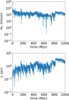 |
Fig. B.1 Core radius (bottom) and core mass (top) for the stellar population of model C05. |
Appendix C Single model distribution of velocity and position
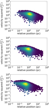 |
Fig. C.1 Distribution of velocity square and relative position of ffcs at t=0 for models C025 (top), C05 (middle), and C075 (bottom). |
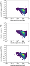 |
Fig. C.2 Distribution of velocity square and relative position of ffcs at 1 Gyr for models C025 (top), C05 (middle), and C075 (bottom). |
Appendix D Escape velocity of stars and ffcs in all models
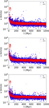 |
Fig. D.1 Speed of escaping ffcs (blue) and stars (red) at 1 Gyr for models C025 (top), C05 (middle), and C075 (bottom). |
Appendix E Velocity dispersion of ffcs
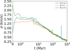 |
Fig. E.1 Velocity dispersion of all ffc in all models. The initial imprint of the velocity distribution of ffc is fastly removed in less than 1 Myr, with all models having similar velocity dispersion around 40 Myr. The spikes shown in the figure are due to high velocity ffc due to a stellar encounter. |
All Tables
All Figures
|
Fig. 1 Evolution of Lagrangian radii enclosing 0.1%, 10%, and 50% of the total mass for stars and percentage of ffcs (indicated in the legend with the virial ratio of the model), for the models C025 (top), C05 (middle), and C075 (bottom). At each time step, the Lagrangian radii were calculated based on the total mass of the star cluster at that time. |
| In the text | |
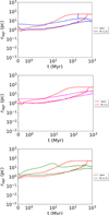 |
Fig. 2 Same as in Figure 1, but for the 50% and 90% Lagrangian radii. |
| In the text | |
|
Fig. 3 Top: evolution of Lagrangian radii containing mass of 0.1% and 10% for both stars and percentage of ffcs from each model. Bottom: same, but for 50% and 90% Lagrangian radii. The Lagrangian radii at each time were calculated using the total mass of the star cluster at that time. |
| In the text | |
|
Fig. 4 Velocity dispersion of stellar population and ffc population. The ffc velocity dispersion is smaller than that of the stellar population in all models. The presented velocity dispersion considers the center of mass for the binary systems. A zoomed-in view of the ffcs’ curves is in Appendix E. |
| In the text | |
|
Fig. 5 Radial positions and square velocities of ffcs, for all simulated models, at t=0 Myr (top panel) and at the end of the simulation at t= 1000 Myr (bottom panel). We also added every single model separately from the rest in Appendix D. |
| In the text | |
|
Fig. 6 Cumulative ejection distribution of escapers, including both stars and ffcs. Notably, the ejection function for all three ffc models shows variation only at the beginning, after which it progresses almost linearly. |
| In the text | |
|
Fig. 7 Relaxation timescale of LMP population for different masses using our initial conditions for the number of LMP and the half-mass radius. The relaxation timescale for an Earth mass and a Jupiter mass are from the red line and green line, respectively. The orange line shows the star limit (i.e., the ignition of hydrogen at ≈ 0.08 M⊙). The red dot shows the timescale considering a mass spectra of LMP in a uniform logarithmic distribution, ranging from Earth mass to Jupiter mass, using the same initial condition of our main models. Finally, the blue line shows results taking into account the initial conditions of the model C05. |
| In the text | |
|
Fig. 8 Mass segregation timescale of LMP population for different masses (left) and number of initial objects (right) using our initial conditions for the number of LMP and the half-mass radius. In the left plot, we show the mass segregation timescale for coupled (MSTc) and decoupled (MSTdc) timescales. MSPEJ is instead the mass segregation timescale for a decoupled mass spectrum from Earth to Jupiter masses, distributed in a logarithmic uniform distribution. On the right, with similar semantics, we have Earth, Jupiter, and a brown dwarf coupled (c suffix) and decoupled (dc suffix). The relaxation timescale for a Jupiter mass and an Earth mass are indicated with the orange and green lines, respectively. |
| In the text | |
|
Fig. 9 Top: Lagrangian radii evolution of both stellar and brown-dwarf components in the 0.1%, 1%, 10%, 50%, and 90% shells. The Lagrangian radii evolution is green for the stellar components and red for the brown dwarfs. Bottom: with identical shells, we display the average mass evolution. |
| In the text | |
|
Fig. B.1 Core radius (bottom) and core mass (top) for the stellar population of model C05. |
| In the text | |
|
Fig. C.1 Distribution of velocity square and relative position of ffcs at t=0 for models C025 (top), C05 (middle), and C075 (bottom). |
| In the text | |
|
Fig. C.2 Distribution of velocity square and relative position of ffcs at 1 Gyr for models C025 (top), C05 (middle), and C075 (bottom). |
| In the text | |
|
Fig. D.1 Speed of escaping ffcs (blue) and stars (red) at 1 Gyr for models C025 (top), C05 (middle), and C075 (bottom). |
| In the text | |
|
Fig. E.1 Velocity dispersion of all ffc in all models. The initial imprint of the velocity distribution of ffc is fastly removed in less than 1 Myr, with all models having similar velocity dispersion around 40 Myr. The spikes shown in the figure are due to high velocity ffc due to a stellar encounter. |
| In the text | |
Current usage metrics show cumulative count of Article Views (full-text article views including HTML views, PDF and ePub downloads, according to the available data) and Abstracts Views on Vision4Press platform.
Data correspond to usage on the plateform after 2015. The current usage metrics is available 48-96 hours after online publication and is updated daily on week days.
Initial download of the metrics may take a while.