| Issue |
A&A
Volume 706, February 2026
|
|
|---|---|---|
| Article Number | A257 | |
| Number of page(s) | 17 | |
| Section | Stellar structure and evolution | |
| DOI | https://doi.org/10.1051/0004-6361/202557390 | |
| Published online | 16 February 2026 | |
The stellar activity-rotation-age relationship under the lens of asteroseismology
1
STAR Institute, Université de Liège Liège, Belgium
2
Department of Physics and Astronomy, Uppsala University Box 516 SE-751 20 Uppsala, Sweden
3
Space Research Institute, Russian Academy of Sciences Profsoyuznaya 84/32 117997 Moscow, Russia
4
Max Planck Institute for Astrophysics Karl-Schwarzschild-Str 1 Garching b. München D-85741, Germany
5
Kazan Federal University 18 Kremlyovskaya Street Kazan, Russia
6
Max-Planck-Institut für Sonnensystemforschung Justus-von-Liebig-Weg 3 37077 Göttingen, Germany
7
Astrophysics Research Center, Keele University Keele ST5 5BG, UK
★ Corresponding author: This email address is being protected from spambots. You need JavaScript enabled to view it.
Received:
24
September
2025
Accepted:
11
December
2025
Abstract
Context. In low-mass stars, the connection between magnetic activity, rotation period, and age provides key insights into the functioning of dynamos. Fully understanding the activity-rotation-age relationship requires access to stars with precise fundamental parameters, measured rotation periods, and reliable magnetic activity indicators (e.g. X-ray luminosity). Thanks to space-based photometry, asteroseismology is now the leading method for determining stellar parameters with unprecedented precision and accuracy. The best-characterised solar-like stars compose the Kepler LEGACY sample, with the highest quality asteroseismic data for 66 stars, most of which have measured rotation periods. In the X-ray band, these stars were observed by the ROentgen Survey with an Imaging Telescope Array (eROSITA) telescope on the Russian Spektrum-Roentgen-Gamma (SRG) satellite in the course of its all-sky survey.
Aims. We reviewed different components of the stellar activity–rotation–age relationship using the largest sample of solar-like stars with highly accurate fundamental parameters from asteroseismology, along with their measured rotation periods and X-ray luminosities.
Methods. We cross-correlated the Kepler LEGACY sample with the SRG/eROSITA source catalogue, finding X-ray detections for 13 of them. We derived their fundamental parameters using the Forward and Inversion COmbination (FICO) procedure and revisited widely studied activity-age and activity-rotation relationships by consistently incorporating our subsample of 13 stars with literature samples.
Results. By implementing revised activity-rotation-age relationships in a star-planet interaction (SPI) code to compute the X-ray luminosity tracks and by comparing the results with observations, we found an improved agreement for seven stars of our subsample. We explored the effect of the revised relationships on the mass loss of planets in the radius valley, finding a modest impact on planet size distributions.
Conclusions. A larger and more varied sample of stars with asteroseismically characterised parameters, rotation period, and activity indicators is needed to accurately determine the multiple components of the activity-rotation-age relationship.
Key words: planet-star interactions / stars: activity / stars: evolution / stars: low-mass / stars: rotation / stars: solar-type
© The Authors 2026
 Open Access article, published by EDP Sciences, under the terms of the Creative Commons Attribution License (https://creativecommons.org/licenses/by/4.0), which permits unrestricted use, distribution, and reproduction in any medium, provided the original work is properly cited.
This article is published in open access under the Subscribe to Open model. This email address is being protected from spambots. You need JavaScript enabled to view it. to support open access publication.
1. Introduction
Studies of the mutual dependence between magnetic activity, rotational period, and age in low-mass stars (defined here as stars with initial mass of M★ ≲ 1.5 M⊙ and spectral types F to M) continues to fuel a growing interest in the scientific community, as these quantities are critical observational proxies of the dynamo operating in stellar convective interiors. The rotational and magnetic properties of low-mass stars are tightly interconnected through a dynamo feedback loop (Vidotto 2021), regulated by competing effects of internal differential rotation, turbulent convection, and braking at the stellar surface by magnetised winds (Parker 1955). According to this feedback loop, as stars evolve, their surface rotation and magnetism globally decrease, resulting in a less powerful dynamo and angular momentum removal.
In this context, many studies have been dedicated to observationally constraining the relationships between stellar surface rotation with age (e.g. Skumanich 1972; Bouvier et al. 1997; Barnes 2003), magnetic activity with age (e.g. Güdel et al. 1997; Preibisch & Feigelson 2005; Telleschi et al. 2005; Booth et al. 2017), and magnetic activity with surface rotation (e.g. Skumanich 1972; Noyes et al. 1984; Wright et al. 2011; Johnstone et al. 2015; Wright et al. 2018; Magaudda et al. 2020). These approaches have been aimed at determining their mutual dependencies across diverse stellar evolutionary stages. Although past studies have been crucially informative on the activity-rotation-age relationship for low-mass stars up to a few billion years, the limited access to accurate ages for older stars has prevented a comprehensive investigation of this relationship for more evolved objects.
Thanks to the advent of space-based photometry missions, such as CoRoT (Baglin et al. 2009), Kepler (Borucki et al. 2010), TESS (Ricker et al. 2014), and K2 (Howell et al. 2014), asteroseismology has established itself as a powerful tool for the derivation of fundamental stellar parameters (age, M★, R★), with an unprecedented level of precision and accuracy. Recent investigations on the rotational period-age relationship (Prot − age) based on asteroseismically characterised stars (van Saders et al. 2016) showed that solar-like stars more evolved than the Sun appear to rotate faster than what is predicted by typical spin-down models (e.g. Matt et al. 2015), hinting at a weakening of the dynamo that would no longer be able to (fully) sustain the activity-rotation-age feedback loop. In this respect, several efforts have been dedicated to investigate the corresponding consequences on the magnetic activity properties (e.g. Booth et al. 2017; Metcalfe et al. 2022, 2024), but the dearth of robust activity indicators for evolved stars has strongly challenged the derivation of comprehensive and exhaustive results.
The stellar X-ray luminosity, Lx, is a fundamental activity indicator, unambiguously associated with the magnetic heating of the plasma in the stellar corona. It has been widely used to calibrate Lx-age and Lx-Prot (or Rx-Ro, where Rx is the ratio between Lx and the bolometric luminosity, Lbol, and Ro is the stellar Rossby number) relationships for younger stars (e.g. see recent works on more than 650 first X-ray detected Pleiades members with eROSITA in Khamitov et al. 2024). Significantly more challenging is studying these relationships in more evolved stars that are intrinsically fainter (Lx ≲ 1027 erg/s), requiring the use of highly sensitive telescopes and long exposure times. Booth et al. (2017) first studied the Lx-age relationship in a sample of 14 old solar-like stars with ages derived by means of more accurate techniques, where asteroseismology was used in six cases. As a result, these authors found a steepening of the activity-age relationship for evolved stars (age ≳ 1 Gyr) compared to their younger counterparts, which appeared to be in contrast to the flattening of the Prot-age relationship observed by van Saders et al. (2016).
To develop a comprehensive picture of the activity-rotation-age relationship for evolved stars, it is crucial to expand the sample of stars that possess accurately determined fundamental parameters, measurements of the rotational period, and X-ray detections. In this study, we revisit the different components of the activity-rotation-age relationship by introducing a stellar sample whose fundamental parameters can be precisely determined through asteroseismic techniques. For this purpose, the Kepler LEGACY sample (Lund et al. 2017), comprising 66 solar-like stars (from late K to early F type) with the highest quality seismic data currently available until the launch of PLATO, represents the most suitable choice. In Sect. 2, we detail the target selection based on the availability of rotational periods (Santos et al. 2021) and the search and analysis of X-ray detections within the ROentgen Survey with an Imaging Telescope Array (eROSITA; Predehl et al. 2021) on board the Russian Spektrum-Roentgen-Gamma mission (SRG; Sunyaev et al. 2021) (SRG/eROSITA-RU) all-sky surveys for stars in the Kepler LEGACY sample. In Sect. 3, we describe our new derivation of the stellar fundamental parameters for our subsample of Kepler LEGACY stars with X-ray detections. In Sect. 4, we revisit the X-ray activity versus age, and X-ray activity versus stellar Rossby number relationships. In Sect. 5, we implement the revisited relationships in theoretical models to compute X-ray luminosity tracks and highlight any potential difference with respect to previous findings. Finally, in Sect. 6, we test the impact of the revisited activity-rotation-age relationships on the evaporation of planetary atmospheres.
2. Target selection and X-ray fluxes from eROSITA
We used the X-ray luminosity of a star as an indicator of its magnetic activity. To this end, we cross-correlated the Kepler LEGACY sample with the SRG/eROSITA source catalogue obtained in the course of its all-sky survey during 2019-20221. The Kepler LEGACY field was observed with SRG/eROSITA for four surveys. We used the 0.3 − 2.3 keV SRG/eROSITA source catalogue derived from full-sky survey data and searched for matches within 98% positional uncertainty of X-ray sources, which was typically in the ∼5 − 15 arcsec range. The SRG/eROSITA matches were filtered by the detection confidence threshold corresponding to 3σ (threshold on the likelihood value of ≥6). The Gaia positions of stars were corrected for the proper motion to bring them to the mean epoch of SRG/eROSITA observations. For further analysis, we only retained the stars with measured rotation periods in Santos et al. (2021). From the global sample of 66 stars from the Kepler LEGACY, we kept 51 stars.
One of the eROSITA sources, SRGe J185621.8+453027, has two objects within its 98% error circle, Gaia DR3 2106822131755292032 and 2106822131756839808, separated by 1.5 and 4.0 arcsec, respectively. We searched for the nature and global properties of the two objects on SIMBAD (Wenger et al. 2000), finding that Gaia DR3 2106822131756839808 corresponds to the Kepler LEGACY star KIC9139163; whereas no correspondence has been found for Gaia DR3 2106822131755292032. By querying the Gaia archive, we found that the G magnitude of Gaia DR3 2106822131755292032 (15.70) is significantly fainter compared to Gaia DR3 2106822131756839808 (8.26). In an attempt to refine the nature of Gaia DR3 2106822131755292032, we searched for photometric estimates from the G magnitude of Teff, log g, and [Fe/H], but we found no data. We computed the X-ray luminosity associated with SRGe J185621.8+453027 firstly deriving the source’s distance from the Gaia DR3 parallax, which was initially corrected for the systematic offset, known as the “parallax zero-point” Groenewegen (2021). It was then used to infer the stellar distances by means of the geometric Bayesian method from Bailer-Jones et al. (2021). We obtained Lx = (9.23 ± 1.15) × 1028 erg/s, a value which appears to be compatible with the X-ray luminosities expected for solar-like star on the main sequence. With the lack of indications on the nature of the Gaia DR3 2106822131755292032 object and the compatibility of the X-ray luminosity of SRGe J185621.8+453027, with the one typically expected for MS solar-like stars, we found it reasonable to associate SRGe J185621.8+453027 to Gaia DR3 2106822131756839808 (KIC9139163).
The X-ray fluxes quoted in the eROSITA catalogue were recalculated for the spectrum of thermal emission of optically thin plasma with a temperature of 150 eV, assuming a zero column of neutral hydrogen in the line of sight, NH = 0, for the same 0.3–2.3 keV energy range. For a temperature of 300 (500) eV, the presented luminosities should be multiplied by a factor of 0.83 (0.81). Moderate values of column density, NH ∼ 1020 cm−2 change these values by a few percent. We did not attempt to apply the bolometric correction of X-ray luminosities because of its potentially large uncertainty. Similarly, conversion of eROSITA fluxes to the ROSAT energy band of 0.1–2.4 keV involves extrapolation to lower energies outside eROSITA working energy band and could be rather uncertain, especially for sources with softer spectra and/or fainter sources having large uncertainties on their coronal temperature. For example, it has a moderate value of ≈1.25 for the plasma temperature of kT = 300 eV and increases towards lower temperatures, reaching the value of ≈2.5 for kT = 150 eV. It is worth keeping this point in mind in the following analysis and in the comparison of the revisited activity-rotation-age relationships with the theoretical X-ray tracks in Sect. 5. The eROSITA detected stars from Kepler LEGACY sample, used for the following analysis are listed in Table 1.
eROSITA detected stars from a subset of Kepler LEGACY sample used in this work.
3. Kepler LEGACY subsample: derivation of the fundamental stellar parameters
To construct our asteroseismic models, we employed the Forward and Inversion COmbination (FICO) procedure (Bétrisey et al. 2022, 2023a, 2024a; Bétrisey 2024), a sophisticated methodology that combines forward modelling with inversion techniques. This approach, rooted in pioneering works by Reese et al. (2012) and Buldgen et al. (2019a), enables a precise and accurate determination of fundamental parameters of solar-like stars, such as mass, radius, and age. Without delving into detail beyond the scope of this article, we highlight that the FICO procedure was notably designed to deal with surface effects, which are among the main limiting factors of asteroseismic characterisation. The FICO method addresses these effects through a three-step strategy. It begins by fitting individual oscillation frequencies using the Ball & Gizon (2014) surface correction. The next step of the procedure consists of a mean density inversion. This inversion, based on Reese et al. (2012), refines the estimate of the mean density in a quasi-model-independent manner. Finally, the frequency separation ratios, computed following Roxburgh & Vorontsov (2003), along with the inverted mean density and the spectroscopic constraints are used for the last optimisation step. Although these ratios are almost insensitive to near-surface inaccuracies (Roxburgh & Vorontsov 2003; Otí Floranes et al. 2005), they also lack information about the stellar mean density; hence, there is a need for the prior inversion step. For a broader overview of seismic inversion techniques and their successful applications, we refer to the review by Buldgen et al. (2022a) and the references therein (see e.g. Di Mauro 2004; Buldgen et al. 2015b,a, 2016a,b, 2017, 2019b,a, 2022b; Kosovichev & Kitiashvili 2020; Salmon et al. 2021; Bétrisey & Buldgen 2022; Bétrisey et al. 2022, 2023b,a; 2024a,b, 2025b,a, for a non-exhaustive selection). The observational constraints are provided in Appendix A.
We used the Asteroseismic Inference on a Massive Scale (AIMS) software (Rendle et al. 2019) to fit individual oscillation frequencies alongside spectroscopic constraints (Teff, [Fe/H], and L), to which an extended version of the Spelaion grid (Bétrisey et al. 2023a) was provided as input. Surface effects were corrected using the formula of Ball & Gizon (2014). The free parameters included mass, age, initial hydrogen and metal mass fractions (X0 and Z0), and surface correction coefficients. For stars above 1.10 M⊙, overshooting was also included as free parameter. Uniform uninformative priors were considered, except for the stellar age, which was uniformly constrained between 0 and 13.8 Gyr. Each AIMS run consisted in a burn-in phase followed by a solution run. The initial fit used 800 walkers, 8000 burn-in steps, and 3000 solution steps. This dense sampling ensured strong convergence, particularly for the surface correction terms.
To ensure the reliability of the final FICO step, especially near the end of the main sequence, where seismic degeneracies increase (e.g. White et al. 2011), we performed an interpolation validation test. This involved regenerating a stellar model using the optimal AIMS parameters and the same evolution and pulsation codes as the original grid. A successful match between the recomputed and interpolated frequencies confirms the physical validity of the AIMS solution. Discrepancies, typically manifesting as age overestimation, indicate interpolation failure and require local re-optimisation. This issue affected a minority of our sample, namely KIC2837475, KIC6508366, and KIC11253226. For these stars, we performed an additional local minimisation using a Levenberg-Marquardt algorithm (e.g. Frandsen et al. 2002; Teixeira et al. 2003; Miglio & Montalbán 2005), optimising the same parameters as in AIMS. Constraints included the r01 ratios, spectroscopic data, the inverted mean density, and the lowest radial-mode frequency. As indicated in Table 2, where the fundamental stellar parameters for the 13 Kepler LEGACY stars are listed, the agreement with the metallicity values in Table A.1 is worse for KIC2837475 and KIC11253226, which is likely the sign of non-standard processes (e.g. turbulent diffusion, undershooting, radiative accelerations; see Deal et al. 2018; Buldgen et al. 2025, and references therein) not included in the standard physics used in our stellar models, especially considering the presence of a strong oscillatory signal in the r01 and r10 ratios. However, the estimated mass, radius, age, and luminosity do not seem to be significantly affected and remain consistent with independent determinations of Silva Aguirre et al. (2017). It is worth noting that our final sample is dominated by F-type stars. This reflects the composition of the global Kepler LEGACY sample, with the majority of stars belonging to the F spectral type. These stars have thinner convective envelopes in comparison to their cooler counterparts, which might reduce the braking efficiency via magnetised winds. Kraft (1967) provided a limit in Teff(K)∼6250 (Kraft break) for the transition between stars with thick enough convective envelopes and efficient braking and stars without (or with very thin) convective envelopes and inefficient braking. In the context of the characterisation of the stellar activity-rotation-age relationship, comparing the properties of our stars with the Kraft break could give an indication about the braking efficiency of these objects. In a recent work, Beyer & White (2024) reassessed the limit of Teff(K) = 6550 ± 200 for the Kraft break, by studying the rotational properties of 405 F-type stars within 33.33 pc. They found that stars above the break have projected velocities of vsin(i) = (61.5 ± 30.6) km/s, while those below have vsin(i) = (6.7 ± 3.6) km/s, with a transition at vsin(i) ≃ 20 km/s. By deriving rotational velocities for our sample of stars (from best-fit stellar models’ radii and measured rotation periods from Santos et al. 2021) and by checking Teff (see Tables 2 and 3), we found that KIC2837475, KIC7103006, KIC11081729, and KIC11253226 could be in the transition region of the Kraft break, but none of our stars clearly lie above it. In general, the actual transition into a regime with inefficient braking and disappearance of the thin convective envelope for stars does not appear to be as sharp in terms of Teff (or equivalently of mass) as the classical Kraft break. On the contrary, this transition would occur over a broader range (M(M⊙)≃1.5 − 2.5), with a strong dependence on several stellar properties (e.g. age, metallicity, internal rotation at birth, angular momentum loss, etc.) (Kawaler 1988; Aerts 2025; Amard & Matt 2020; Amard et al. 2020). Given the uncertainties related with the properties of the dynamos and magnetic fields for the stars in this regime, in the following analysis, we compare the results obtained by including the whole sample of stars, on the one hand, and by removing the hottest stars, on the other.
Fundamental stellar parameters from asteroseismic modelling.
Rotational periods, equatorial velocities, colours, and Rossby numbers for our sample of Kepler LEGACY stars.
In Fig. 1, we show the distribution of the evolutionary tracks in the Hertzsprung-Russell diagram (HRD). Among the 13 stars analysed here, KIC8006161 represents the nearest solar analogue, despite its larger metallicity. In the following sections, the relative position of this star compared to the solar one is highlighted to visualise any significant impact due to higher metallicity.
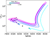 |
Fig. 1. HRD showing the best-fit models’ tracks of the 13 Kepler LEGACY stars with X-ray detections. The location of the Sun in the L/L⊙ vs Teff(K) plane is shown as reference. |
4. Study of the activity-rotation-age relationship
After determining both the X-ray luminosities (see Sect. 2) and the fundamental parameters (see Sect. 3) for our sample of 13 solar-like stars, we studied the relationships linking the stellar magnetic activity with the age and with the rotational period or dynamo efficiency by means of the Rossby number. This latter quantity is defined as Ro = Prot/τconv, where Prot is the surface rotational period and τconv is the convective turnover timescale; namely, the timescale needed for a convective bubble to travel from the base to a certain height within the convective regions. Several methods have been proposed to determine this non-observable quantity at different heights within convective envelopes, which are usually linked to the stellar colours or effective temperatures (e.g. Noyes et al. 1984; Wright et al. 2011; Cranmer & Saar 2011). In this work, we computed τconv with two approaches. The first one follows the empirically derived prescription of Wright et al. (2018) that is based on the stellar (V − Ks)0 colour and is valid for 1.1 < (V − Ks)0 < 7. We determined this last quantity by taking the V and Ks magnitudes from SIMBAD (Wenger et al. 2000), and computed (V − Ks)0 = (V − Ks)+(−AV + AKs), where AKs = 0.161 × E(B − V) is derived from the 3D dustmaps for Galactic reddening (Green et al. 2018), and AV = 3.1 × E(B − V) (Savage & Mathis 1979). Notably, Table 3 shows that the (V − Ks)0 colours for KIC2837475, KIC9139163, KIC11081729, and KIC11253226 are slightly below the lower limit required for applying the prescription of Wright et al. (2018). In this case, the τconv is potentially overestimated, as indicated by Fig. 7 in Wright et al. (2011). The second approach follows the parametrisation of zero age main sequence (ZAMS) stellar models from Gunn et al. (1998) by Cranmer & Saar (2011), which is valid for 3300 ≲ Teff (K) ≲ 7000. To compute τconv with this second approach, we used the effective temperature values in Table 2. A comparison between the convective turnover timescales computed with the approaches mentioned above for each target is shown in Fig. B.1. For the sake of completeness, we computed τconv at the base of the convective zone derived from best-fit stellar models in Table 2, by adopting the convention of Montesinos et al. (2001). We include their values in Fig. B.1. The corresponding Rossby numbers for the three diverse approaches are listed in Table 3, while in Fig. B.2, we compare their values, which are consistently normalised by the solar one (Ro⊙, (V − Ks)0 = 2.306, Ro⊙, Teff = 1.95, Ro⊙, m = 2.19). We recall that for the calibration of the activity-rotation-age relationships, we used the first and second approach to compute τconv.
With all the key quantities determined for our sample of stars, we studied its impact on some relationships which have been intensively investigated in the literature to provide key indications on the evolution of stellar activity as a function of the age and Rossby number:  (e.g. Booth et al. 2017), log(Rx) − log(age) (e.g. Jackson et al. 2012), and log(Rx)−log(Ro) (e.g. Wright et al. 2011; Magaudda et al. 2020; Johnstone et al. 2021), with Rx = Lx/Lbol. In the following, we present the methodology and results obtained when revisiting these relationships.
4.1. Log(Lx/R2) versus log(age)
Booth et al. (2017, hereafter B17) calibrated the activity-age relationship by considering a sample of 14 stars older than about 1 Gyr and X-ray detections from either Chandra or XMM-Newton observations. For 6 out of 14 stars (i.e. 16 CygA, Proxima Cen, Alpha CenB, KIC7529180, KIC9955598, and KIC10016239) the ages have been asteroseismically determined. With this sample of stars, they performed an orthogonal distance regression to fit the decimal logarithm of the X-ray luminosity normalised to the stellar radius versus the decimal logarithm of the age, with the units of the three quantities above given in erg/s, solar radii, and years, respectively. They found a relatively steep linear dependence, taking the form
 (1)
(1)
In our work, we revisited this relationship by joining our 13 Kepler LEGACY stars to the 6 stars of B17 with asteroseismically derived ages. For consistency with respect to the method used to determine the stellar age, we decided to not include the rest of the B17 sample. Since the X-ray luminosities in B17 were calculated in the 0.2–2.0 keV energy band to ensure a more consistent analysis and comparison with respect to the X-ray theoretical tracks computed in Sect. 5, we converted their X-ray fluxes into the ROSAT energy band (0.1–2.4 keV) by means of the WebPIMMS2 tool. We first rescaled the X-ray fluxes in B17 with updated distances from Gaia EDR3. We thus provided the rescaled fluxes as input to WebPIMMS assuming an APEC model with solar abundance and uniform coronal temperature, log(T(K)) = 6.50 (Booth et al. 2017). We also include the Sun among our sample of stars. In this case, we took the Lx from Wright et al. (2011) and the relative uncertainty from B17. The X-ray luminosities derived from the converted fluxes of the B17 subsample are indicated in Table C.1.
With this final sample of 20 stars (including the Sun), we performed an orthogonal distance regression on log(Lx/R2)-log(age), with a weighted linear fit, by means of the SciPy ODR method (Virtanen et al. 2020), finding
 (2)
(2)
where the uncertainties on the fitting parameters are expressed as one standard deviation. To test the goodness of the fit we computed the reduced chi-squared, χred2 = 26.9. This value clearly indicates a poor fit, which is mostly due to the very scattered distribution of the points in the log(Lx/R2)-log(age) plane, as shown in Fig. 2.
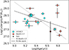 |
Fig. 2. Distribution of 13 stars from the Kepler LEGACY (cyan dots) and 7 stars from B17 (orange pentagons) including the Sun (indicated by the usual symbol) in the log(Lx/R2)-log(age) plane. The empty square highlights the position of KIC8006161. The dotted blue and dashed black lines show the fit obtained in B17 and in this work, respectively. |
If we want to make a comparison with the fit found in B17, we can see that a flatter slope is obtained in our case. It is worth noticing that the average age of the stars considered in B17 for the fit is approximately 5 Gyr, which is about twice the one relative to our sample of 20 stars (∼2.5 Gyr). As indicated by van Saders et al. (2016), low-mass stars more evolved than a certain stage may transition into a ‘weakened magnetic braking regime’ (wmb), as a result of an efficiency loss of the dynamo that sustains the stellar magnetic field. This transition may occur whenever the stellar Rossby number becomes larger than a certain threshold value Rocri (e.g. Rocri = (0.92 ± 0.01) Ro⊙, where Ro⊙ is the Sun’s Rossby number, Metcalfe et al. 2024). In this scenario, the stellar spin-down slows considerably, resulting in the stalling of the surface rotational period as stars age. Understanding the consequences for magnetic activity is challenging, given that evolved stars are generally less active, hindering the identification of a possible transition into a diverse regime. By comparing the Rossby number of our 13 Kepler LEGACY stars in Table 3 with respect to Rocri (which is 2.4 or 1.9 for τconv computed as in Wright et al. (2018) or Cranmer & Saar (2011), respectively), we get that in the first case only one star would have already transitioned into the wmb regime; while in the second case, seven stars have Ro larger than 1.9. Similarly, if we compare the Rossby number of the additional six stars from B17 with the two values of Rocri, in both cases we get that only two stars would have transitioned into a wmb regime. Therefore, despite the fact that the B17 stars in Table C.1 have older ages on average, from a magnetic activity point of view, they populate a similar parameter space with respect to the 13 Kepler LEGACY stars at the turn between the potential transition. In this context, while the findings in B17 suggest a steepening of the activity-age relationship in evolved low-mass stars compared to their younger counterparts (e.g. Jackson et al. 2012), our results indicate a more compatible trend. This result is in agreement with the recent work of Aldarondo Quiñones et al. (2025), where the authors derived a shallower slope compared to previous findings.
It is important to note that the uncertainties on the fitting parameters obtained by means of the orthogonal distance regression in the case of a very sparse sample of objects, as the one analysed here, may be significantly underestimated. To derive more robust estimates we implemented a bootstrapping method on the basis of the SciPy ODR, and used a resampling with replacement approach for 25 000 iterations. As a result, we obtained
 (3)
(3)
where the parameters’ values and relative uncertainties indicate the mean and standard deviation of the distribution of best-fitting slopes and intercepts over the total number of iterations. The larger uncertainties found with the bootstrapping method further demonstrate that it is not possible to constrain the  relationship with our global sample of well-characterised 20 stars. Clearly, a statistically more significant number of targets is needed to derive a more precise relationship, and to investigate whether different magnetic activity regimes can be unambiguously identified. In Appendix D, we show the results obtained by excluding stars with Teff(K) > 6250 from the fit, finding a similar mean value for the slope of the relationship and more degraded quality of the fit.
In the following section, we describe our study of the activity-age relationship in a broader context and our attempt to break it down by investigating its dependence on the stellar bolometric luminosity and internal structure properties (as τconv).
4.2. Log(Rx) versus log(age)
To explore the dependence of the activity-age relationship with respect to mass in late-type stars, Jackson et al. (2012, hereafter J12) selected 717 stars from 13 open clusters (α-Persei, Blanco 1, Hyades, IC2391, IC2602, NGC1039, NGC2516, NGC2547, NGC3532, NGC6475, NGC6530, Pleiades, and Praesepe). They split the sample into seven (B − V)0 colour bins, with 0.29 ≤ (B − V)0 < 1.41. By fitting a broken power law in the log(Rx)-log(age) plane, and assuming a constant slope in the saturated regime, they found a decreasing trend of the X-ray-to-bolometric luminosity ratio at saturation (log(Rx,sat)) across the (B − V)0 range, from 10−3.15 to 10−4.28. They further identified saturation-regime turn-off ages consistent with a scatter around ∼100 Myr, this time without a clear trend with respect to the stellar mass.
In our work, we revisited the log(Rx)-log(age) relationship by employing a similar approach to J12, with additional data from our global sample of 20 stars (13 from the Kepler LEGACY, 6 from B17 and the Sun). As a first step, we updated the cluster ages by considering more recent estimates from Bossini et al. (2019) for α-Persei, Blanco 1, IC2391, IC2602, NGC1039, NGC2516, NGC2547, NGC3532, NGC6475, and NGC6530. For NGC6530, we kept the age estimate in J12 and updated the uncertainties by accounting for the work of Prisinzano et al. (2019). Similarly, for Hyades, Pleiades and Praesepe we updated the uncertainties by accounting for the spread in age estimates in Gossage et al. (2018). We updated as well the stellar distances, which were inferred using the geometric Bayesian method described by Bailer-Jones et al. (2021), which accounts for parallax measurement uncertainties and the spatial distribution of stars, using Gaia EDR3 data. Given the significant uncertainties in the distance estimates of the NGC6530 components, we decided to exclude this cluster from the fitting procedure.
Differently from J12, we adopted non-binned data to perform the fit, to consistently account for the contribution of clusters and single stars. The total range of variation for the (B − V)0 colour is slightly larger than the one in J12 ([0.29, 1.83)), to include Proxima Cen. We adopted the SciPy ODR method (Virtanen et al. 2020) to fit the following piecewise linear curve,
 (4)
(4)
where we considered log(Rx, sat), α, and τsat as free parameters, while t is the stellar age. The resulting parameters obtained from the fit on the whole sample of stars are: log(Rv,sat) = −3.55 ± 0.03, α = −1.65 ± 0.11; log(τsat) = 8.15 ± 0.04. The associated χred2 = 19.74 shows also in this case that the scatter of the points hinders the precision of the fit. In Fig. E.1, we show the distribution of stars on the log(Rx)-log(age(yr)) plane with the corresponding fit, indicated by the black dashed line.
To investigate the dependence of Eq. (4) on the stellar mass, or equivalently on the (B − V)0 colour, we split the sample into nine bins, and carried out the same fitting as described above. In Fig. E.2, we show the distribution of stars for each bin with the relative fit, while in Table 4, the corresponding results are listed. From Fig. E.3, we observe that log(Rx,sat) shows a non-decreasing trend as (B − V)0 increases; whereas log(τsat) and α show a quasi-specular behaviour for 0.290 ≤ (B − V)0 ≤ 0.675, with global maximum (minimum) around (B − V)0 ∼ 0.6, while they both increase for (B − V)0 > 0.675. By comparing our results with the one in J12, we firstly highlight the different methods (ODR here and a modified Fasano & Vio (1988) in J12) and number of (B − V)0 colour bins adopted for the fit. We decided to split the global sample in nine instead of seven bins in an attempt to better explore the properties of the Kepler LEGACY stars, whose (B − V)0 colours (in particular) cluster in the range 0.29–0.565. If we compare the α indexes in absolute values, ours tend to be smaller in 0.290 ≤ (B − V)0 < 0.450, 0.790 ≤ (B − V)0 < 0.935 and (B − V)0 ≥ 1.275, while they are larger in the rest of the bins. To test the impact of stars with Teff(K) > 6250, we re-performed the fitting procedure described above by excluding these stars. The results found in this case appear compatible with the ones discussed in this section for the whole sample.
In Sect. 5, we compare and discuss the X-ray luminosity tracks computed by following the results in J12 and those found in this work.
4.3. Log(Rx) versus log(Ro)
After examining how our sample of stars with asteroseismically derived ages influences the relationship between stellar X-ray luminosity and age, we analyzed the relationship between X-ray luminosity and Rossby number. In particular, we studied the impact on the log(Rx)-log(Ro) relationship, which has been widely investigated in the literature (e.g. Wright et al. 2011, 2018; Johnstone et al. 2021).
As in the previous section, we considered a sample of stars for which this relationship has been thoroughly explored in past studies, which is that of Wright et al. (2011, hereafter W11). To this sample, we added the M-dwarf stars from Wright et al. (2018, hereafter W18), the 13 Kepler LEGACY stars analysed in this work, and the sample from B17 listed in Table C.1. To ensure a consistent investigation across the whole sample, we updated and recomputed some quantities in the W11 catalogue; specifically, we updated the stellar distances by adopting Gaia DR3 parallaxes with the Bailer-Jones et al. (2021) method and rescaled the X-ray luminosities accordingly. We computed bolometric luminosities on the basis of the 2MASS Ks magnitude and (V − Ks)0 colours as described above. Additionally, we searched for Teff, log g, and [Fe/H] estimates in Gaia DR3; specifically, from the GSP-Phot module that derives the parameters using low-resolution BP/RP spectra, Gaia photometry, and parallaxes (Andrae et al. 2023; Gaia Collaboration 2023). For most of the stars in the W11 catalogue (94%), we found a match in Gaia DR3. To get more reliable estimates of Teff, log g, and [Fe/H], we also searched into the Apache Point Observatory Galactic Evolution Experiment catalogue (APOGEE, Majewski et al. 2017; Abdurro’uf et al. 2022), where the parameters determination is based on high-resolution spectroscopic data. Nevertheless, we found a match only for 31% of the stars. Therefore, we decided to adopt the parameters derived from the Gaia GSP-Phot method for our analysis. Finally, we cleaned the revised W11 sample by filtering on Gaia astrometric and photometric quality flags, retaining sources with RUWE < 1.4, ipd_frac_multi_peak ≤ 1, rv_amplitude_robust > 9, and G magnitude < 11 (Gossage et al. 2025). The cleaned and revised W11 sample amount to 411 stars.
We attempted a revision analogous to the one of W11 for the sample in W18. Nevertheless, in this case, we found that Gaia GSP-Phot parameters were available only for 2 out of 16 stars with X-ray detections. We thus preferred to keep the Rx estimates of W18, while we retrieved the Teff values from Gaidos et al. (2014) for LSPM J0617+8353, Hejazi et al. (2020) for GJ 699, Hejazi et al. (2022) for LSPM J0024+2626 and LSPM J2012+0112, Kuznetsov et al. (2019) for GJ 3253, Mas-Buitrago et al. (2024) for GJ 3323 and GJ 1256, Kumar et al. (2023) for GJ 3417, Perdelwitz et al. (2024) for GJ 754, Antoniadis-Karnavas et al. (2024) for GJ 551, Jahandar et al. (2025) for GJ 1286, and Wang et al. (2022) for LSPM J0501+2237, respectively.
With this revised global sample of stars, we proceeded with the fit of a piecewise linear curve, of the form
 (5)
(5)
where Rosat represents the value of the Rossby number separating the saturated and unsaturated regimes.
To compute the Rossby number, it is necessary to get an estimate of the convective turnover timescale (τconv). In this work, we considered the prescription of W18, based on the (V − Ks)0 colour and that of Cranmer & Saar (2011), based on the effective temperature. Both methods provide an estimate of the convective turnover timescale at the base of the convective zone, but the correspondence between the two is not homogeneous; thus, using one or the other approach in the fitting procedure may lead to different results. We chose to perform two fits of Eq. (5), one with Ro(V − Ks)0 and one with RoTeff, by means of the SciPy curve_fit method (Virtanen et al. 2020), where we considered a, b, c, and log(Rosat) as free parameters. Since the majority of the stars with asteroseismically characterised ages analysed in this work have spectral types of F and G, we further split our global sample of stars applying a cut in Teff ≥ 3700 K, to separate M-dwarfs from FGK stars. We studied the results of the fit with respect to a relatively more restricted range of spectral types. The results relative to these fitting procedures are presented in Table 5. As expected, depending on the prescription used for the computation of τconv, the fitted parameters assume different values, with the most significant differences found for log(Rosat). The cut in Teff has a major impact on the fit procedure based on RoTeff: in particular, while the slope marked ‘a’ in the saturated regime is negative when the whole sample is considered, it becomes positive (in average value) for the restricted sample. The slope ‘b’ instead becomes steeper in the unsaturated regime. In Figs. 3 and 4, the distribution of stars in the log(Rx)-log(Ro) plane are shown, for τconv computed on the basis of (V − Ks)0 and Teff, respectively, together with the result of the fit indicated by the dashed black line. For each figure, both the results obtained by considering the whole, or restricted sample of stars are presented. Also for the log(Rx)-log(Ro), we tested the impact of removing Kepler LEGACY stars with Teff(K) > 6250 from the fitting procedure. Our results (see Appendix F) were comparable to those described above.
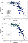 |
Fig. 3. Stars in the log(Rx)-log(Ro) plane, with colour-coded symbols according to the (V − Ks)0 colour. Ro is computed with τconv as in W18. The empty square shows the position of KIC8006161. The black dashed line shows the fit to the stars. Stars with spectral types from M to F are shown in the top panel, while stars from K to F are shown in the bottom one. |
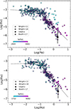 |
Fig. 4. Stars in the log(Rx)-log(Ro) plane, with colour-coded symbols according to Teff. The meanings of symbols and lines are the same as for Fig. 3. |
We also investigated how the log(Rx)-log(Ro) relationship depends on stellar metallicity [Fe/H]. For the stars in W11 and B17, we adopted the [Fe/H] values from Gaia DR3, while for the Kepler LEGACY sample we used the values listed in Table 2. Since most stars from W18 lack metallicity measurements in Gaia DR3, we decided to not include them in this part of the analysis. We divided the overall sample into four metallicity bins spanning a range −1.5 ≤ [Fe/H] ≤ 0.5, selected to ensure a statistically meaningful number of stars in each bin (N = 80 for −1.5 ≤ [Fe/H] < −0.5, N = 131 for −0.5 ≤ [Fe/H] < −0.25, N = 141 for −0.25 ≤ [Fe/H] < 0.0, and N = 80 for 0.0 ≤ [Fe/H] < 0.5), while covering the full range of metallicity variations. The results of this fitting procedure are presented in Table 6, while in Figs. G.1 and G.2 we show the distribution of stars and the linear fit in the log(Rx)-log(Ro) planes for each [Fe/H] bin, for the two computations of the Rossby numbers considered in this work. By looking at the trend of the fitting parameters ‘a’, ‘b’, ‘c’, and log(Rosat) as a function of the metallicity bins in Figs. G.3 and G.4, it is possible to notice that the slope of the log(Rx)-log(Ro) relationship in the saturated regime (‘c’) is steeper in the −1.5 ≤ [Fe/H] < −0.5 bin, especially in the computation with RoTeff for which a correspondingly smaller value of log(Rosat) is observed. For the remaining parameters, it is challenging to establish a clear trend with respect to the metallicity bins, given the significant uncertainties obtained from the fitting procedure.
5. Implementation in theoretical models
In this section, we compare predictions by theoretical models with the measured surface rotational period (or rotation rate) and X-ray luminosity for our sample of Kepler LEGACY stars. In particular for the X-ray luminosity, we present a comparison between the tracks computed by following the revisited log(Rx)-log(Ro) found here and the ones obtained by recalibrating the prescription of Johnstone et al. (2021) as in Pezzotti et al. (2021).
For the computation of the models, we initially derived structural evolutionary tracks for each star in the LEGACY sample by means of the Liège Stellar Evolution Code (CLES Scuflaire et al. 2008) using the optimal stellar parameters derived in Sect. 3, with the same input physics. Subsequently, we provided these structural tracks as input to a star-planet interaction (SPI) code (Privitera et al. 2016; Rao et al. 2018, 2021; Pezzotti et al. 2021, 2025) to simulate the evolution of surface rotation rate and X-ray luminosity, whose properties strongly depend on the characteristics of the input structural tracks. In the SPI code, the evolution of the stellar surface rotation rate is computed under the assumption of solid body rotation, by accounting for the braking at the stellar surface due to magnetised winds as in Matt et al. (2015, 2019), with solar calibrated parameters. Given the degeneracy in the rotational history of solar-like, low-mass stars, we considered initial values of the surface rotation rate (Ωin) ranging between 3.2 and 18 times the surface rotation rate of the Sun (Eggenberger et al. 2019) at solar age (Ω⊙ = 2.9 × 10⁻⁶ s−1) to account for the spread observed for stars in young clusters and stellar associations (Gallet & Bouvier 2015). We assumed disc-locking timescales of 2 and 6 Myr for 10 ≤ Ωin/Ω⊙ ≤ 18, and Ωin/Ω⊙ < 10, respectively.
In the top panel of Fig. 5, an example of surface rotational evolution is shown for KIC 8006161, the nearest solar analogue of our Kepler LEGACY sample, where the yellow region indicates the area included between the 3.2 and 18 Ω⊙ tracks, the gray area shows a further 20% variation with respect to the slow and fast rotator tracks, and finally the blue marker indicates the observational data. In this figure, it can be seen that the measured rotation rate (Santos et al. 2021, S21 in the following) is slightly higher than the one predicted by the Ωin = 18Ω⊙ track, but it is compatible with the gray area. In Fig. 6, we collect the results for all the stars, showing a comparison between the tracks and the measured rotation rate at the stellar age. From this figure, we see that seven stars tend to rotate more slowly than what is predicted by models, while for the remaining six, the tracks are compatible with observational data. It is worth noticing that for the computation of the rotational tracks we have not considered the transition into a weakened magnetic braking regime for Rossby numbers larger than Rocri, where τconv is computed as in Cranmer & Saar (2011). Despite a few stars having Rossby numbers larger than the critical value (Rocri), according to our models, the assumption of a weakening of the magnetic braking is not necessary to reconcile theoretical models with observational data. On the contrary, the inclusion of this mechanism would increase the discrepancy with measured rotational periods.
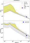 |
Fig. 5. Evolution of the surface rotation rate (top) and X-ray luminosity (bottom) of KIC 8006161. The yellow shaded areas indicate the region explored by the tracks across the evolution of the star, for 3.2 ≤ Ωin/Ω⊙ ≤ 18. The gray shaded areas show 20% (top) and global one order of magnitude (bottom) further variation at the limit of the yellow areas, to account for deviations from more likely rotational histories and fluctuation in the X-ray luminosity due to cyclic or stochastic magnetic activity. The red-dashed line in the top panel shows the evolution of the critical rotation rate, defined as the limit at which the centrifugal acceleration at the equator equals gravity. The blue markers show observational data. For comparison, evolutionary tracks for a 1 M⊙ star are showed, with observational data from Table C.1. |
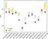 |
Fig. 6. Comparison between theoretical tracks and observational data for the surface rotation rates of stars in Table 2. |
For the computation of the X-ray luminosity tracks, the SPI code includes by default the prescription of Jackson et al. (2012) and Johnstone et al. (2021), which we recalibrated in Pezzotti et al. (2021) according to our computation of Ro. To these two prescriptions, we added their revisited versions; namely, Eq. (4), Table 4 for log(Rx)-log(age) and Eq. (5) and Table 5 for log(Rx)-log(Ro). Our aim was to consistently compare the X-ray luminosity tracks and test the compatibility with observational data. In the bottom panel of Fig. 5, an example of the tracks computed with the recalibrated prescription of Johnstone et al. (2021) is presented and compared with the e-ROSITA X-ray luminosity for KIC 8006161. The yellow area in this figure corresponds to the region explored by the tracks, relatively to different rotational histories. At the extreme of the yellow region, we assumed a further variation of one order of magnitude, that stars may experience because of cyclic (as for the Sun) or stochastic activity.
In Fig. 7, we present the comparison between observational data and X-ray luminosity tracks computed by following the original prescription in J12 (top panel) and the revisited version derived in this work (bottom panel). Thanks to the revisited relationship, a higher compatibility between the tracks and observational data is retrieved in the bottom panel for seven stars (KIC 2837475, KIC 6508366, KIC 7206837, KIC 7940546, KIC 9139163, KIC 9812850, KIC 11081729), while for KIC 7103006 a lower compatibility was obtained. Similarly, in Fig. 8 we present the comparison between observational data and X-ray luminosity tracks computed by using the recalibrated prescription of Johnstone et al. (2021) (top panel), and the revisited version found in this work (bottom panel). Also in this case, we observe that a higher compatibility between tracks and observational data was retrieved, as seen in the bottom panel for four stars (KIC 7206837, KIC 9139163, KIC 9812850, and KIC 11081729).
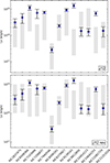 |
Fig. 7. Comparison between theoretical tracks computed with the original prescription of J12 (top panel) and its revisited version (this work, bottom) and observational data for stars in Table 2. |
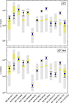 |
Fig. 8. Comparison between theoretical tracks computed with the recalibrated prescription of J21 (top) and its revisited version (this work, bottom) and observational data for stars in Table 2. |
The improvement in the overlap between theoretical tracks and observational data given by the revisited log(Rx)-log(age) and log(Rx)-log(Ro) relationships is not totally surprising, since we directly included data for the Kepler LEGACY stars in the fitting procedures. Despite the relatively small size of our sample of well-characterised stars, that tends to populate the more evolved region of the unsaturated regime generally characterised by a scarcity of data, it provides an important contribution in shaping its properties.
6. Impact on planetary atmospheric mass loss
We investigated and compared the impact of implementing in our SPI code the revisited relationships in Eqs. (4) and (5) on the computation of the planetary mass loss, by computing a set of 1520 models for each considered prescription: ‘J12’ for Jackson et al. (2012), ‘J12 rev’ for the revision of this work, ‘J21’ for Pezzotti et al. (2021), and ‘J21 rev’ for the revision of this work. We selected a set of initial inputs aimed at exploring the properties of the ‘radius valley’ (Fulton et al. 2017), a bimodal size distribution of planets peaked at ∼1.3 and ∼2.4 R⊕ revealed by the Kepler survey, whose nature can be related to atmospheric mass loss, together with other mechanisms (e.g. Venturini et al. 2020; Burn et al. 2024; Nielsen et al. 2015). Our set of initial inputs is: orbital distance 0.1 ≤ ain(AU) ≤ 1.05, in steps of 0.05 AU; planetary core mass 2 ≤ Mcore(M⊕)≤10, in steps of 0.1 M⊕; percentage of primordial atmosphere fixed at 5% of the total planetary mass; 1 M⊙ parent star, with age range from the PMS to 4.57 Gyr, Z = Z⊙, (B − V)0 = 0.656, and initial surface rotation rate fixed at Ωin = 5 Ω⊙.
For the estimation of the mass loss, we used the analytical formulae of Kubyshkina & Fossati (2021). The stellar EUV flux that is given as input to these formulae is computed by rescaling the X-ray luminosity as in Sanz-Forcada et al. (2011) for J12 and J12 rev, and the X-ray flux as in Johnstone et al. (2021) for the J21 and J21 rev relationships. The evolution of the planetary radius was computed by means of the parametrised formula of Lopez & Fortney (2014) for planets with rocky cores and H-He rich gaseous envelopes.
The results of the simulations are collected in Fig. H.1 where we compare the size distribution of planets obtained when using J12 and J12 rev, and J21 and J21 rev, for radius bins from 1.1 to 3.1 R⊕, in steps of 0.1. From these figures we deduce that using the revised prescriptions does not significantly impact the location of the valley, which could shift by one bin between the revised and non-revised prescription. Nevertheless, a maximum difference of 5 and 15 planets was found for the [3.0, 3.1) bin, indicating that using the revised prescriptions yields a difference, albeit a modest one with respect to the simulations analysed here.
7. Summary and conclusions
We revisited different components of the activity-rotation-age relationship by introducing the largest sample of solar-like stars with the highest quality asteroseismic data, surface rotational periods, and X-ray detections. We studied the log(Lx/R2)-log(age) relationship finding that the fitting procedure is hindered by the very scattered distributions of stars and the low statistics. By comparing the average value of the slope with the results in Booth et al. (2017), we found indications of a flatter linear dependence.
We recalibrated the log(Rx)-log(age) relationship by joining our sample of well-characterised stars to the one in Jackson et al. (2012). We recomputed the slopes in the saturated and unsaturated regimes for the global and split samples of stars in nine (B − V)0 colour bins. We recalibrated the log(Rx)-log(Ro) relationship by first considering the whole spectral range and then by applying a cut on spectral type from K to F. The major impact on the fitting parameters due to the cut is recovered for Rossby numbers, or convective turnover timescales, computed on the basis of Teff. We further analysed this relationship by splitting the sample into [Fe/H] bins, finding that relatively more metal-poor stars tend to follow a steeper slope in the unsaturated regime.
We finally implemented the revisited relationships for log(Rx)-log(age) and log(Rx)-log(Ro) in our SPI code to compute rotational and X-ray luminosity tracks for the 13 Kepler LEGACY stars analysed in this work. By comparing the rotational tracks computed without weakened magnetic braking with measured rotational periods, we notice that our stars on average tend to rotate more slowly than what is predicted by the models. This result shows that the hypothesis of a weakened magnetic braking taking over for Ro ≥ Rocri is not strictly necessary in our case. By comparing the X-ray tracks computed with the relationships found in this work and the ones in the literature with luminosities from eROSITA, we found that the revisited relationships provide improved agreement for a good fraction of the sample. To test the impact of the revisited relationships on the mass loss from planetary atmospheres, we simulated the evaporation of planets in the radius valley, accounting for a 1 M⊙ parent star, with properties analogous to those of our Sun. By comparing the size distribution of planets obtained with the revisited and non-revisited prescriptions, we observe the major difference for the bin with the largest radius. This difference, however, appears modest when compared to the total number of planets involved in the simulation.
Larger samples of stars with well-characterised parameters, rotation period, and activity indicators are needed to accurately determine the multiple components of the activity-rotation-age relationship. In this context, asteroseismology will play a crucial role in releasing precise characterisations for thousands of stars with the advent of PLATO.
Acknowledgments
We thank the anonymous referee for useful comments that helped to improve the quality of this manuscript. This work used data of eROSITA telescope onboard SRG observatory. The SRG observatory was built by Roskosmos in the interests of the Russian Academy of Sciences represented by its Space Research Institute (IKI) in the framework of the Russian Federal Space Program, with the participation of the Deutsches Zentrum für Luft- und Raumfahrt (DLR). The SRG/eROSITA X-ray telescope was built by a consortium of German Institutes led by MPE, and supported by DLR. The SRG spacecraft was designed, built, launched and is operated by the Lavochkin Association and its subcontractors. The science data are downlinked via the Deep Space Network Antennae in Bear Lakes, Ussurijsk, and Baykonur, funded by Roskosmos. The eROSITA data used in this work were processed using the eSASS software system developed by the German eROSITA consortium and proprietary data reduction and analysis software developed by the Russian eROSITA Consortium. CP thanks the Belgian Federal Science Policy Office (BELSPO) for the financial support in the framework of the PRODEX Program of the European Space Agency (ESA) under contract number 4000141194. JB acknowledges funding from the SNF Postdoc. Mobility grant no. P500PT_222217 (Impact of magnetic activity on the characterisation of FGKM main-sequence host-stars). MG, IB acknowledge support by the RSF grant N 23-12-00292. GB is funded by the Fonds National de la Recherche Scientifique (FNRS).
References
- Abdurro’uf, Accetta, K., Aerts, C., et al. 2022, ApJS, 259, 35 [NASA ADS] [CrossRef] [Google Scholar]
- Aerts, C. 2025, A&A, 704, A332 [NASA ADS] [CrossRef] [EDP Sciences] [Google Scholar]
- Aldarondo Quiñones, N., Jenkins, S., Vanderburg, A., Soares-Furtado, M., & McDonald, M. A. 2025, PASP, 137, 114206 [Google Scholar]
- Amard, L., & Matt, S. P. 2020, ApJ, 889, 108 [Google Scholar]
- Amard, L., Roquette, J., & Matt, S. P. 2020, MNRAS, 499, 3481 [NASA ADS] [CrossRef] [Google Scholar]
- Andrae, R., Fouesneau, M., Sordo, R., et al. 2023, A&A, 674, A27 [CrossRef] [EDP Sciences] [Google Scholar]
- Antoniadis-Karnavas, A., Sousa, S. G., Delgado-Mena, E., Santos, N. C., & Andreasen, D. T. 2024, A&A, 690, A58 [NASA ADS] [CrossRef] [EDP Sciences] [Google Scholar]
- Baglin, A., Auvergne, M., Barge, P., et al. 2009, in Transiting Planets, eds. F. Pont, D. Sasselov, & M. J. Holman, IAU Symp., 253, 71 [NASA ADS] [Google Scholar]
- Bailer-Jones, C. A. L., Rybizki, J., Fouesneau, M., Demleitner, M., & Andrae, R. 2021, AJ, 161, 147 [Google Scholar]
- Ball, W. H., & Gizon, L. 2014, A&A, 568, A123 [NASA ADS] [CrossRef] [EDP Sciences] [Google Scholar]
- Barnes, S. A. 2003, ApJ, 586, 464 [Google Scholar]
- Barnes, S. A. 2007, ApJ, 669, 1167 [Google Scholar]
- Bétrisey, J. 2024, Ph.D. Thesis, University of Geneva, Switzerland [Google Scholar]
- Bétrisey, J., & Buldgen, G. 2022, A&A, 663, A92 [NASA ADS] [CrossRef] [EDP Sciences] [Google Scholar]
- Bétrisey, J., Pezzotti, C., Buldgen, G., et al. 2022, A&A, 659, A56 [NASA ADS] [CrossRef] [EDP Sciences] [Google Scholar]
- Bétrisey, J., Buldgen, G., Reese, D. R., et al. 2023a, A&A, 676, A10 [NASA ADS] [CrossRef] [EDP Sciences] [Google Scholar]
- Bétrisey, J., Eggenberger, P., Buldgen, G., Benomar, O., & Bazot, M. 2023b, A&A, 673, L11 [NASA ADS] [CrossRef] [EDP Sciences] [Google Scholar]
- Bétrisey, J., Buldgen, G., Reese, D. R., & Meynet, G. 2024a, A&A, 681, A99 [NASA ADS] [CrossRef] [EDP Sciences] [Google Scholar]
- Bétrisey, J., Farnir, M., Breton, S. N., et al. 2024b, A&A, 688, L17 [NASA ADS] [CrossRef] [EDP Sciences] [Google Scholar]
- Bétrisey, J., Broomhall, A. M., Breton, S. N., et al. 2025a, A&A, 699, L9 [NASA ADS] [CrossRef] [EDP Sciences] [Google Scholar]
- Bétrisey, J., Reese, D. R., Breton, S. N., et al. 2025b, A&A, 697, A219 [Google Scholar]
- Beyer, A. C., & White, R. J. 2024, ApJ, 973, 28 [Google Scholar]
- Booth, R. S., Poppenhaeger, K., Watson, C. A., Silva Aguirre, V., & Wolk, S. J. 2017, MNRAS, 471, 1012 [NASA ADS] [CrossRef] [Google Scholar]
- Borucki, W. J., Koch, D., Basri, G., et al. 2010, Science, 327, 977 [Google Scholar]
- Bossini, D., Vallenari, A., Bragaglia, A., et al. 2019, A&A, 623, A108 [NASA ADS] [CrossRef] [EDP Sciences] [Google Scholar]
- Bouvier, J., Forestini, M., & Allain, S. 1997, A&A, 326, 1023 [NASA ADS] [Google Scholar]
- Buldgen, G., Reese, D. R., & Dupret, M. A. 2015a, A&A, 583, A62 [NASA ADS] [CrossRef] [EDP Sciences] [Google Scholar]
- Buldgen, G., Reese, D. R., Dupret, M. A., & Samadi, R. 2015b, A&A, 574, A42 [NASA ADS] [CrossRef] [EDP Sciences] [Google Scholar]
- Buldgen, G., Reese, D. R., & Dupret, M. A. 2016a, A&A, 585, A109 [NASA ADS] [CrossRef] [EDP Sciences] [Google Scholar]
- Buldgen, G., Salmon, S. J. A. J., Reese, D. R., & Dupret, M. A. 2016b, A&A, 596, A73 [NASA ADS] [CrossRef] [EDP Sciences] [Google Scholar]
- Buldgen, G., Reese, D., & Dupret, M.-A. 2017, Eur. Phys. J. Web Conf., 160, 03005 [NASA ADS] [CrossRef] [EDP Sciences] [Google Scholar]
- Buldgen, G., Farnir, M., Pezzotti, C., et al. 2019a, A&A, 630, A126 [EDP Sciences] [Google Scholar]
- Buldgen, G., Rendle, B., Sonoi, T., et al. 2019b, MNRAS, 482, 2305 [Google Scholar]
- Buldgen, G., Bétrisey, J., Roxburgh, I. W., Vorontsov, S. V., & Reese, D. R. 2022a, Front. Astron. Space Sci., 9, 942373 [NASA ADS] [CrossRef] [Google Scholar]
- Buldgen, G., Farnir, M., Eggenberger, P., et al. 2022b, A&A, 661, A143 [NASA ADS] [CrossRef] [EDP Sciences] [Google Scholar]
- Buldgen, G., Bétrisey, J., Pezzotti, C., Borisov, S., & Noels, A. 2025, A&A, 702, A162 [NASA ADS] [CrossRef] [EDP Sciences] [Google Scholar]
- Burn, R., Mordasini, C., Mishra, L., et al. 2024, Nat. Astron., 8, 463 [Google Scholar]
- Casagrande, L., & VandenBerg, D. A. 2014, MNRAS, 444, 392 [Google Scholar]
- Casagrande, L., & VandenBerg, D. A. 2018, MNRAS, 475, 5023 [Google Scholar]
- Cranmer, S. R., & Saar, S. H. 2011, ApJ, 741, 54 [Google Scholar]
- Deal, M., Alecian, G., Lebreton, Y., et al. 2018, A&A, 618, A10 [NASA ADS] [CrossRef] [EDP Sciences] [Google Scholar]
- Di Mauro, M. P. 2004, in SOHO 14 Helio- and Asteroseismology: Towards a Golden Future, ed. D. Danesy, ESA Spec. Pub., 559, 186 [NASA ADS] [Google Scholar]
- Eggenberger, P., Buldgen, G., & Salmon, S. J. A. J. 2019, A&A, 626, L1 [NASA ADS] [CrossRef] [EDP Sciences] [Google Scholar]
- Fasano, G., & Vio, R. 1988, Bulletin d’Information du Centre de Donnees Stellaires, 35, 191 [Google Scholar]
- Frandsen, S., Carrier, F., Aerts, C., et al. 2002, A&A, 394, L5 [NASA ADS] [CrossRef] [EDP Sciences] [Google Scholar]
- Fulton, B. J., Petigura, E. A., Howard, A. W., et al. 2017, AJ, 154, 109 [Google Scholar]
- Furlan, E., Ciardi, D. R., Cochran, W. D., et al. 2018, ApJ, 861, 149 [Google Scholar]
- Gaia Collaboration (Brown, A. G. A., et al.) 2021, A&A, 649, A1 [NASA ADS] [CrossRef] [EDP Sciences] [Google Scholar]
- Gaia Collaboration (Vallenari, A., et al.) 2023, A&A, 674, A1 [NASA ADS] [CrossRef] [EDP Sciences] [Google Scholar]
- Gaidos, E., Mann, A. W., Lépine, S., et al. 2014, MNRAS, 443, 2561 [Google Scholar]
- Gallet, F., & Bouvier, J. 2015, A&A, 577, A98 [NASA ADS] [CrossRef] [EDP Sciences] [Google Scholar]
- Gossage, S., Conroy, C., Dotter, A., et al. 2018, ApJ, 863, 67 [Google Scholar]
- Gossage, S., Kiman, R., Monsch, K., et al. 2025, ApJ, 988, 102 [Google Scholar]
- Green, G. M., Schlafly, E. F., Finkbeiner, D., et al. 2018, MNRAS, 478, 651 [Google Scholar]
- Groenewegen, M. A. T. 2021, A&A, 654, A20 [NASA ADS] [CrossRef] [EDP Sciences] [Google Scholar]
- Güdel, M., Guinan, E. F., & Skinner, S. L. 1997, ApJ, 483, 947 [Google Scholar]
- Gunn, A. G., Mitrou, C. K., & Doyle, J. G. 1998, MNRAS, 296, 150 [Google Scholar]
- Hejazi, N., Lépine, S., Homeier, D., Rich, R. M., & Shara, M. M. 2020, AJ, 159, 30 [NASA ADS] [CrossRef] [Google Scholar]
- Hejazi, N., Lépine, S., & Nordlander, T. 2022, ApJ, 927, 122 [NASA ADS] [CrossRef] [Google Scholar]
- Howell, S. B., Sobeck, C., Haas, M., et al. 2014, PASP, 126, 398 [Google Scholar]
- Jackson, A. P., Davis, T. A., & Wheatley, P. J. 2012, MNRAS, 422, 2024 [Google Scholar]
- Jahandar, F., Doyon, R., Artigau, É., et al. 2025, ApJ, 978, 154 [Google Scholar]
- Johnstone, C. P., Güdel, M., Stökl, A., et al. 2015, ApJ, 815, L12 [Google Scholar]
- Johnstone, C. P., Bartel, M., & Güdel, M. 2021, A&A, 649, A96 [EDP Sciences] [Google Scholar]
- Kawaler, S. D. 1988, ApJ, 333, 236 [Google Scholar]
- Khamitov, I. M., Bikmaev, I. F., Gilfanov, M. R., Sunyaev, R. A., & Medvedev, P. S. 2024, Astron. Lett., 50, 780 [Google Scholar]
- Kosovichev, A. G., & Kitiashvili, I. N. 2020, in Solar and Stellar Magnetic Fields: Origins and Manifestations, eds. A. Kosovichev, S. Strassmeier, & M. Jardine, 354, 107 [NASA ADS] [Google Scholar]
- Kraft, R. P. 1967, ApJ, 150, 551 [Google Scholar]
- Kubyshkina, D. I., & Fossati, L. 2021, Res. Notes Am. Astron. Soc., 5, 74 [Google Scholar]
- Kumar, V., Rajpurohit, A. S., Srivastava, M. K., Fernández-Trincado, J. G., & Queiroz, A. B. A. 2023, MNRAS, 524, 6085 [Google Scholar]
- Kuznetsov, M. K., del Burgo, C., Pavlenko, Y. V., & Frith, J. 2019, ApJ, 878, 134 [Google Scholar]
- Lindegren, L., Bastian, U., Biermann, M., et al. 2021, A&A, 649, A4 [EDP Sciences] [Google Scholar]
- Lopez, E. D., & Fortney, J. J. 2014, ApJ, 792, 1 [Google Scholar]
- Lund, M. N., Silva Aguirre, V., Davies, G. R., et al. 2017, ApJ, 835, 172 [Google Scholar]
- Magaudda, E., Stelzer, B., Covey, K. R., et al. 2020, A&A, 638, A20 [NASA ADS] [CrossRef] [EDP Sciences] [Google Scholar]
- Majewski, S. R., Schiavon, R. P., Frinchaboy, P. M., et al. 2017, AJ, 154, 94 [NASA ADS] [CrossRef] [Google Scholar]
- Mas-Buitrago, P., González-Marcos, A., Solano, E., et al. 2024, A&A, 687, A205 [NASA ADS] [CrossRef] [EDP Sciences] [Google Scholar]
- Matt, S. P., Brun, A. S., Baraffe, I., Bouvier, J., & Chabrier, G. 2015, ApJ, 799, L23 [Google Scholar]
- Matt, S. P., Brun, A. S., Baraffe, I., Bouvier, J., & Chabrier, G. 2019, ApJ, 870, L27 [Google Scholar]
- Metcalfe, T. S., Finley, A. J., Kochukhov, O., et al. 2022, ApJ, 933, L17 [NASA ADS] [CrossRef] [Google Scholar]
- Metcalfe, T. S., Strassmeier, K. G., Ilyin, I. V., et al. 2024, ApJ, 960, L6 [NASA ADS] [CrossRef] [Google Scholar]
- Miglio, A., & Montalbán, J. 2005, A&A, 441, 615 [NASA ADS] [CrossRef] [EDP Sciences] [Google Scholar]
- Montesinos, B., Thomas, J. H., Ventura, P., & Mazzitelli, I. 2001, MNRAS, 326, 877 [NASA ADS] [CrossRef] [Google Scholar]
- Nielsen, M. B., Schunker, H., Gizon, L., & Ball, W. H. 2015, A&A, 582, A10 [NASA ADS] [CrossRef] [EDP Sciences] [Google Scholar]
- Noyes, R. W., Hartmann, L. W., Baliunas, S. L., Duncan, D. K., & Vaughan, A. H. 1984, ApJ, 279, 763 [Google Scholar]
- Otí Floranes, H., Christensen-Dalsgaard, J., & Thompson, M. J. 2005, MNRAS, 356, 671 [CrossRef] [Google Scholar]
- Parker, E. N. 1955, ApJ, 122, 293 [Google Scholar]
- Perdelwitz, V., Trifonov, T., Teklu, J. T., Sreenivas, K. R., & Tal-Or, L. 2024, A&A, 683, A125 [NASA ADS] [CrossRef] [EDP Sciences] [Google Scholar]
- Pezzotti, C., Eggenberger, P., Buldgen, G., et al. 2021, A&A, 650, A108 [NASA ADS] [CrossRef] [EDP Sciences] [Google Scholar]
- Pezzotti, C., Buldgen, G., Magaudda, E., et al. 2025, A&A, 694, A179 [NASA ADS] [CrossRef] [EDP Sciences] [Google Scholar]
- Pinsonneault, M. H., An, D., Molenda-Żakowicz, J., et al. 2012, ApJS, 199, 30 [Google Scholar]
- Predehl, P., Andritschke, R., Arefiev, V., et al. 2021, A&A, 647, A1 [EDP Sciences] [Google Scholar]
- Preibisch, T., & Feigelson, E. D. 2005, ApJS, 160, 390 [NASA ADS] [CrossRef] [Google Scholar]
- Prisinzano, L., Damiani, F., Kalari, V., et al. 2019, A&A, 623, A159 [NASA ADS] [CrossRef] [EDP Sciences] [Google Scholar]
- Privitera, G., Meynet, G., Eggenberger, P., et al. 2016, A&A, 593, A128 [NASA ADS] [CrossRef] [EDP Sciences] [Google Scholar]
- Rao, S., Meynet, G., Eggenberger, P., et al. 2018, A&A, 618, A18 [NASA ADS] [CrossRef] [EDP Sciences] [Google Scholar]
- Rao, S., Pezzotti, C., Meynet, G., et al. 2021, A&A, 651, A50 [NASA ADS] [CrossRef] [EDP Sciences] [Google Scholar]
- Reese, D. R., Marques, J. P., Goupil, M. J., Thompson, M. J., & Deheuvels, S. 2012, A&A, 539, A63 [NASA ADS] [CrossRef] [EDP Sciences] [Google Scholar]
- Rendle, B. M., Buldgen, G., Miglio, A., et al. 2019, MNRAS, 484, 771 [Google Scholar]
- Ricker, G. R., Winn, J. N., Vanderspek, R., et al. 2014, in Space Telescopes and Instrumentation 2014: Optical, Infrared, and Millimeter Wave, eds. J. Oschmann, M. Jacobus, M. Clampin, G. G. Fazio, & H. A. MacEwen, SPIE Conf. Ser., 9143, 914320 [Google Scholar]
- Roxburgh, I. W., & Vorontsov, S. V. 2003, A&A, 411, 215 [NASA ADS] [CrossRef] [EDP Sciences] [Google Scholar]
- Salmon, S. J. A. J., Van Grootel, V., Buldgen, G., Dupret, M. A., & Eggenberger, P. 2021, A&A, 646, A7 [NASA ADS] [CrossRef] [EDP Sciences] [Google Scholar]
- Santos, A. R. G., Breton, S. N., Mathur, S., & García, R. A. 2021, ApJS, 255, 17 [NASA ADS] [CrossRef] [Google Scholar]
- Sanz-Forcada, J., Micela, G., Ribas, I., et al. 2011, A&A, 532, A6 [NASA ADS] [CrossRef] [EDP Sciences] [Google Scholar]
- Savage, B. D., & Mathis, J. S. 1979, ARA&A, 17, 73 [NASA ADS] [CrossRef] [Google Scholar]
- Scuflaire, R., Théado, S., Montalbán, J., et al. 2008, Ap&SS, 316, 83 [Google Scholar]
- Silva Aguirre, V., Lund, M. N., Antia, H. M., et al. 2017, ApJ, 835, 173 [Google Scholar]
- Skumanich, A. 1972, ApJ, 171, 565 [Google Scholar]
- Sunyaev, R., Arefiev, V., Babyshkin, V., et al. 2021, A&A, 656, A132 [NASA ADS] [CrossRef] [EDP Sciences] [Google Scholar]
- Teixeira, T. C., Christensen-Dalsgaard, J., Carrier, F., et al. 2003, Ap&SS, 284, 233 [NASA ADS] [CrossRef] [Google Scholar]
- Telleschi, A., Güdel, M., Briggs, K., et al. 2005, ApJ, 622, 653 [Google Scholar]
- van Saders, J. L., Ceillier, T., Metcalfe, T. S., et al. 2016, Nature, 529, 181 [Google Scholar]
- Venturini, J., Guilera, O. M., Haldemann, J., Ronco, M. P., & Mordasini, C. 2020, A&A, 643, L1 [NASA ADS] [CrossRef] [EDP Sciences] [Google Scholar]
- Vidotto, A. A. 2021, Liv. Rev. Sol. Phys., 18, 3 [Google Scholar]
- Virtanen, P., Gommers, R., Oliphant, T. E., et al. 2020, Nat. Med., 17, 261 [Google Scholar]
- Wang, Y.-F., Luo, A. L., Chen, W.-P., et al. 2022, A&A, 660, A38 [NASA ADS] [CrossRef] [EDP Sciences] [Google Scholar]
- Wenger, M., Ochsenbein, F., Egret, D., et al. 2000, A&AS, 143, 9 [NASA ADS] [CrossRef] [EDP Sciences] [Google Scholar]
- White, T. R., Bedding, T. R., Stello, D., et al. 2011, ApJ, 743, 161 [Google Scholar]
- Wright, N. J., Drake, J. J., Mamajek, E. E., & Henry, G. W. 2011, ApJ, 743, 48 [Google Scholar]
- Wright, N. J., Newton, E. R., Williams, P. K. G., Drake, J. J., & Yadav, R. K. 2018, MNRAS, 479, 2351 [Google Scholar]
The Kepler field resides in the half of the sky reserved to the Russian eROSITA consortium. We invite interested readers to directly contact the members of the consortium for information about data availability.
Appendix A: Observational constraints for the asteroseismic characterisations
We used the acoustic oscillation frequencies from Lund et al. (2017) as seismic constraints. The spectroscopic constraints were taken from Furlan et al. (2018), except for KIC8379927 for which we used the data from Pinsonneault et al. (2012). The absolute stellar luminosity was derived using
 (A.1)
(A.1)
where λ is the wavelength band. Specifically, we used the 2MASS Ks-band, except for KIC10454113 for which we used the 2MASS H-band, given the very large uncertainty in the Ks-band. In this equation, mλ is the apparent magnitude, BCλ is the bolometric correction computed following Casagrande & VandenBerg (2014, 2018), d is the distance in pc from Gaia EDR3 (Gaia Collaboration 2021), Aλ is the extinction computed with the dust map from Green et al. (2018), and Mbol,⊙ = 4.75 is the absolute solar bolometric magnitude. The distance was estimated using two approaches, either by inverting the parallax corrected according to Lindegren et al. (2021) or by using the distance from Bailer-Jones et al. (2021). Both methods led to similar distances and we adopted the distance from Bailer-Jones et al. (2021) for our final luminosities. The spectroscopic constraints and luminosities are summarised in Table A.1.
Observational constraints for the asteroseismic characterisations.
Appendix B: Comparison of different prescription for the computation of τconv
In Fig. B.1, we show a comparison between the convective turnover timescales computed with the prescriptions from Wright et al. (2018), Cranmer & Saar (2011), and from best-fit stellar models using the convention of Montesinos et al. (2001) for the 13 Kepler LEGACY stars in Table 2. With respect to the first approach, we notice that the (V−Ks)0 colour of KIC2837475 and KIC11253226 lies below the validity limit for the Wright et al. (2018) prescription, causing an overestimation of τconv. In Fig. B.2, we show the normalised Rossby number with respect to the solar one for τconv computed by means of the three approaches mentioned above. For τconv computed as in Wright et al. (2018), Ro/R⊙ < 1 for all stars, except for KIC8006161. For τconv computed as in Cranmer & Saar (2011), six out of thirteen stars have Ro/R⊙ < 1. Finally, for τconv computed from our best-fit stellar models, only three stars have Ro/R⊙ < 1. It is worth recalling that for the computation of the theoretical surface rotation rate and X-ray luminosity tracks with our SPI in Sect. 5, we used the prescription of Cranmer & Saar (2011) to compute τconv.
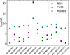 |
Fig. B.1. Comparison among the convective turnover timescales computed for the 13 stars of the Kepler LEGACY sample with the prescription from Wright et al. (2018) (cyan dots), Cranmer & Saar (2011) (magenta dots) and from the asteroseismic models (lime dots) with the Montesinos et al. (2001) convention. |
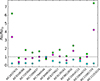 |
Fig. B.2. Comparison among normalised Rossby numbers with respect the Rossby number of the Sun for the 13 stars of the Kepler LEGACY sample, with convective turnover timescale computed as in Wright et al. (2018) (cyan dots), Cranmer & Saar (2011) (magenta dots), and from the asteroseismic models (lime dots) with the Montesinos et al. (2001) convention. |
Appendix C: Subsample of stars from Booth et al. (2017)
In Table C.1, we indicate the quantities of interest for the present study relatively to the subsample of stars with asteroseismically determined ages extracted from Booth et al. (2017).
Fundamental quantities for the subsample of seven stars extracted from Booth et al. (2017), including the Sun.
Appendix D: Log(Lx/R2) versus log(age) for stars with Teff(K) ≤ 6250
We performed the fit of the log(Lx/R2) versus log(age) relationship by excluding stars with Teff(K) > 6250, that could be above the Kraft break. We found the resulting fit,
 (D.1)
(D.1)
with reduced  . We further applied a bootstrap method as described in Sect. 4.1, finding
 (D.2)
(D.2)
In Fig. D.1, the distribution of stars in the log(Lx/R2) versus log(age) plane and the fit are showed.
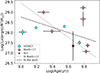 |
Fig. D.1. Distribution of stars from the Kepler LEGACY (cyan dots) with Teff ≤ 6250 and stars from B17 (orange pentagons) including the Sun (indicated by the usual symbol) in the log(Lx/R2)-log(age) plane. |
Appendix E: Log(Rx)-log(age) fit dependence on (B−V)0
In Figs. E.1 and E.2, the fit of the log(Rx)-log(age) relationship is represented for the global and split ranges of the stellar (B−V)0 colour, respectively. In Fig. E.3, the trends of the fitting parameters are indicated, as a function of the (B−V)0 colour bins. We also studied the impact of removing stars with Teff(K) > 6250 from the fitting procedure, finding a negligible impact.
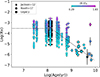 |
Fig. E.1. Distribution of stars in the log(Rx)-log(age) plane, where the star, dot and pentagon markers indicate targets from J12, Kepler LEGACY, and B17, respectively. The empty square highlights the position of KIC8006161. The black dashed line indicates the fit of Eq. 4. Data are colour coded according to (B−V)0. |
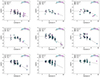 |
Fig. E.2. Fit of the log(Rx)-log(age) relationship divided by (B−V)0 colour bin. The meaning of the symbols is the same one as in Fig. E.1. |
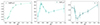 |
Fig. E.3. Trends of the fitting parameters listed in Table 4, along with log(Rx,sat), log(τsat), and α as function of the (B−V)0 colour bin, shown from left to right. |
Appendix F: Log(Rx)-log(Ro) relationship for Kepler LEGACY stars with Teff(K) ≤ 6250
In Table F.1 we present the results obtained in the fitting procedure on the log(Rx)-log(Ro) relationship when excluding stars with Teff(K) > 6250.
Results of the fitting procedure determined with an analogous procedure to Table 5, but for Kepler LEGACY stars with Teff(K) ≤ 6250.
Appendix G: Log(Rx)-log(Ro) fit dependence on [Fe/H]
In Figs. G.1 and G.2, we show the fit of the Log(Rx)-Log(Ro) relationship for the global sample of stars divided in four metallicity bins, for τconv computed as in Wright et al. (2018) and Cranmer & Saar (2011), respectively. In Figs. G.3 and G.4, the relative trend of the characteristic parameters of the fits are showed.
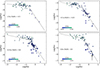 |
Fig. G.1. Distributions of stars from W11 (star symbols), Kepler LEGACY (dots), and B17 (pentagons) in the Log(Rx)–Log(Ro) plane, split in four metallicity bins, with [Fe/H] increasing from left to right, top to bottom. Ro is computed as in W18, and the stars are colour coded according to (V−Ks)0. |
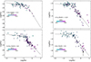 |
Fig. G.2. Distributions of stars from W11 (star symbol), Kepler LEGACY (dots), and B17 (pentagons) in the Log(Rx)–Log(Ro) plane, split in four metallicity bins, with [Fe/H] increasing from left to right, top to bottom. Ro is computed as in Cranmer & Saar (2011), and the stars are colour coded according to Teff. |
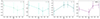 |
Fig. G.3. Trends of the fitting parameters listed in Table 6 (a, b, c) and log(Rosat) as a function of the metallicity bin, for Ro computed as in W18, shown from left to right. |
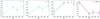 |
Fig. G.4. Trends of the fitting parameters listed in Table 6 (a, b, c) and log(Rosat) as a function of the metallicity bin, for Ro computed as in Cranmer & Saar (2011), shown from left to right. |
Appendix H: Impact of recalibrated prescriptions on planetary mass loss
In Fig. H.1 we show the comparison between the number of planets per radius bin obtained when using J12 and J12 rev, and analogously J21 and J21 rev prescriptions in our SPI code for the computation of the X-ray luminosity tracks.
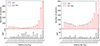 |
Fig. H.1. Left: Comparison between the number of planets per radius bin at 4.57 Gyr, obtained by simulating the atmospheric mass loss due to the X-ray luminosity computed with the original prescription of Jackson et al. (2012) (blue bars) and the revisited one (this work, red bars) and EUV irradiation as in Sanz-Forcada et al. (2011), for a 1 M⊙ parent star at solar metallicity. In the bottom panel, the numerical difference (in modulus) of planets per bin for the two considered prescriptions is shown. Right: Meaning of the plot is the same as for the left panel, but for the recalibrated prescription of Johnstone et al. (2021) as in Pezzotti et al. (2021) (blue bars) and the revisited one (this work, red bars). |
All Tables
Rotational periods, equatorial velocities, colours, and Rossby numbers for our sample of Kepler LEGACY stars.
Fundamental quantities for the subsample of seven stars extracted from Booth et al. (2017), including the Sun.
Results of the fitting procedure determined with an analogous procedure to Table 5, but for Kepler LEGACY stars with Teff(K) ≤ 6250.
All Figures
|
Fig. 1. HRD showing the best-fit models’ tracks of the 13 Kepler LEGACY stars with X-ray detections. The location of the Sun in the L/L⊙ vs Teff(K) plane is shown as reference. |
| In the text | |
|
Fig. 2. Distribution of 13 stars from the Kepler LEGACY (cyan dots) and 7 stars from B17 (orange pentagons) including the Sun (indicated by the usual symbol) in the log(Lx/R2)-log(age) plane. The empty square highlights the position of KIC8006161. The dotted blue and dashed black lines show the fit obtained in B17 and in this work, respectively. |
| In the text | |
|
Fig. 3. Stars in the log(Rx)-log(Ro) plane, with colour-coded symbols according to the (V − Ks)0 colour. Ro is computed with τconv as in W18. The empty square shows the position of KIC8006161. The black dashed line shows the fit to the stars. Stars with spectral types from M to F are shown in the top panel, while stars from K to F are shown in the bottom one. |
| In the text | |
|
Fig. 4. Stars in the log(Rx)-log(Ro) plane, with colour-coded symbols according to Teff. The meanings of symbols and lines are the same as for Fig. 3. |
| In the text | |
|
Fig. 5. Evolution of the surface rotation rate (top) and X-ray luminosity (bottom) of KIC 8006161. The yellow shaded areas indicate the region explored by the tracks across the evolution of the star, for 3.2 ≤ Ωin/Ω⊙ ≤ 18. The gray shaded areas show 20% (top) and global one order of magnitude (bottom) further variation at the limit of the yellow areas, to account for deviations from more likely rotational histories and fluctuation in the X-ray luminosity due to cyclic or stochastic magnetic activity. The red-dashed line in the top panel shows the evolution of the critical rotation rate, defined as the limit at which the centrifugal acceleration at the equator equals gravity. The blue markers show observational data. For comparison, evolutionary tracks for a 1 M⊙ star are showed, with observational data from Table C.1. |
| In the text | |
|
Fig. 6. Comparison between theoretical tracks and observational data for the surface rotation rates of stars in Table 2. |
| In the text | |
|
Fig. 7. Comparison between theoretical tracks computed with the original prescription of J12 (top panel) and its revisited version (this work, bottom) and observational data for stars in Table 2. |
| In the text | |
|
Fig. 8. Comparison between theoretical tracks computed with the recalibrated prescription of J21 (top) and its revisited version (this work, bottom) and observational data for stars in Table 2. |
| In the text | |
|
Fig. B.1. Comparison among the convective turnover timescales computed for the 13 stars of the Kepler LEGACY sample with the prescription from Wright et al. (2018) (cyan dots), Cranmer & Saar (2011) (magenta dots) and from the asteroseismic models (lime dots) with the Montesinos et al. (2001) convention. |
| In the text | |
|
Fig. B.2. Comparison among normalised Rossby numbers with respect the Rossby number of the Sun for the 13 stars of the Kepler LEGACY sample, with convective turnover timescale computed as in Wright et al. (2018) (cyan dots), Cranmer & Saar (2011) (magenta dots), and from the asteroseismic models (lime dots) with the Montesinos et al. (2001) convention. |
| In the text | |
|
Fig. D.1. Distribution of stars from the Kepler LEGACY (cyan dots) with Teff ≤ 6250 and stars from B17 (orange pentagons) including the Sun (indicated by the usual symbol) in the log(Lx/R2)-log(age) plane. |
| In the text | |
|
Fig. E.1. Distribution of stars in the log(Rx)-log(age) plane, where the star, dot and pentagon markers indicate targets from J12, Kepler LEGACY, and B17, respectively. The empty square highlights the position of KIC8006161. The black dashed line indicates the fit of Eq. 4. Data are colour coded according to (B−V)0. |
| In the text | |
|
Fig. E.2. Fit of the log(Rx)-log(age) relationship divided by (B−V)0 colour bin. The meaning of the symbols is the same one as in Fig. E.1. |
| In the text | |
|
Fig. E.3. Trends of the fitting parameters listed in Table 4, along with log(Rx,sat), log(τsat), and α as function of the (B−V)0 colour bin, shown from left to right. |
| In the text | |
|
Fig. G.1. Distributions of stars from W11 (star symbols), Kepler LEGACY (dots), and B17 (pentagons) in the Log(Rx)–Log(Ro) plane, split in four metallicity bins, with [Fe/H] increasing from left to right, top to bottom. Ro is computed as in W18, and the stars are colour coded according to (V−Ks)0. |
| In the text | |
|
Fig. G.2. Distributions of stars from W11 (star symbol), Kepler LEGACY (dots), and B17 (pentagons) in the Log(Rx)–Log(Ro) plane, split in four metallicity bins, with [Fe/H] increasing from left to right, top to bottom. Ro is computed as in Cranmer & Saar (2011), and the stars are colour coded according to Teff. |
| In the text | |
|
Fig. G.3. Trends of the fitting parameters listed in Table 6 (a, b, c) and log(Rosat) as a function of the metallicity bin, for Ro computed as in W18, shown from left to right. |
| In the text | |
|
Fig. G.4. Trends of the fitting parameters listed in Table 6 (a, b, c) and log(Rosat) as a function of the metallicity bin, for Ro computed as in Cranmer & Saar (2011), shown from left to right. |
| In the text | |
|
Fig. H.1. Left: Comparison between the number of planets per radius bin at 4.57 Gyr, obtained by simulating the atmospheric mass loss due to the X-ray luminosity computed with the original prescription of Jackson et al. (2012) (blue bars) and the revisited one (this work, red bars) and EUV irradiation as in Sanz-Forcada et al. (2011), for a 1 M⊙ parent star at solar metallicity. In the bottom panel, the numerical difference (in modulus) of planets per bin for the two considered prescriptions is shown. Right: Meaning of the plot is the same as for the left panel, but for the recalibrated prescription of Johnstone et al. (2021) as in Pezzotti et al. (2021) (blue bars) and the revisited one (this work, red bars). |
| In the text | |
Current usage metrics show cumulative count of Article Views (full-text article views including HTML views, PDF and ePub downloads, according to the available data) and Abstracts Views on Vision4Press platform.
Data correspond to usage on the plateform after 2015. The current usage metrics is available 48-96 hours after online publication and is updated daily on week days.
Initial download of the metrics may take a while.