| Issue |
A&A
Volume 706, February 2026
|
|
|---|---|---|
| Article Number | A105 | |
| Number of page(s) | 13 | |
| Section | Stellar structure and evolution | |
| DOI | https://doi.org/10.1051/0004-6361/202557437 | |
| Published online | 03 February 2026 | |
Formation of the dormant black holes with luminous companions from binary or triple systems
1
School of Physical Science and Technology, Xinjiang University Urumqi 830046, China
2
Xinjiang Astronomical Observatory, Chinese Academy of Sciences 150 Science 1-Street Urumqi Xinjiang 830011, China
3
Institute for Experimental and Theoretical Physics, Al-Farabi Kazakh National University Almaty 050040, Kazakhstan
★ Corresponding authors: This email address is being protected from spambots. You need JavaScript enabled to view it.
; This email address is being protected from spambots. You need JavaScript enabled to view it.
; This email address is being protected from spambots. You need JavaScript enabled to view it.
Received:
26
September
2025
Accepted:
29
November
2025
Abstract
Context. Recently, a class of dormant black hole (BH) binaries with luminous companions (dBH-LCs) has been observed, such as Gaia BH1, BH2, and BH3. Unlike previously discovered X-ray BH binaries, the observed dBH-LCs have relatively long orbital periods (typically more than several tens to a few hundred days) and show very weak X-ray emission.
Aims. Studying the formation and evolution of the whole dBH-LC population is a very interesting problem. Our aim is to study the contribution of massive stars to the dBH-LC population under different evolutionary models, namely, isolated binary evolution (IBE) and hierarchical triple evolution, and different formation channels (i.e., mass transfer and common envelope evolution).
Methods. Using the Massive Objects in Binary Stellar Evolution code, the Triple Stellar Evolution code, and the latest initial multiple-star distributions, we modeled the populations of massive stars. We then calculated the orbital properties, mass distributions, and birth rates of the dBH-LC populations formed under these different conditions.
Results. In the Milky Way, we calculate that the birth rate of dBH-LCs formed through IBE is about 4.35 × 10⁻⁵ yr−1, while the birth rate through triple evolution is about 1.47 × 10⁻³ yr−1. This means that the birth rate from triple evolution is one to two orders of magnitude higher than that from IBE. We find that in triple evolution, the main formation channel of dBH-LCs is post-merger binaries formed from inner binary mergers triggered by von Zeipel−Lidov−Kozai oscillations. In particular, if the merger product is formed from a central helium-burning star and a main-sequence star, the resulting star usually has a small core mass and a large envelope mass. The stars with this structure can form BHs in the pair-instability supernova range (about 60 M⊙ ∼ 120 M⊙), and they are about three times more massive than the maximum BH mass formed through IBE.
Conclusions. Due to the presence of dynamical effects in triple evolution, the inner binaries in triples are more likely to interact than isolated binaries. As a result, dBH-LCs formed through triple evolution mainly come from the channel where the inner binary merges. The birth rate of dBH-LCs from triple evolution is about two orders of magnitude higher than that from IBE. In addition, some dBH-LCs with heavy BHs are also formed through the inner binary merger channel in triples. These results strongly indicate that the triple evolution can be the most important channel for dBH-LC formation.
Key words: binaries: close / stars: black holes / stars: evolution
© The Authors 2026
 Open Access article, published by EDP Sciences, under the terms of the Creative Commons Attribution License (https://creativecommons.org/licenses/by/4.0), which permits unrestricted use, distribution, and reproduction in any medium, provided the original work is properly cited.
This article is published in open access under the Subscribe to Open model. This email address is being protected from spambots. You need JavaScript enabled to view it. to support open access publication.
1. Introduction
It is estimated that the Milky Way (MW) contains about 108 stellar-mass black holes (BHs; Brown & Bethe 1994; Timmes et al. 1996). These BHs may exist in single-star systems, binary systems, or multiple-star systems (McClintock & Remillard 2006; Remillard & McClintock 2006; Qian et al. 2008; Bodensteiner et al. 2020; Wang & Zhu 2021; Sahu et al. 2025). In the past, BHs with luminous companions (LCs) were usually discovered using radio and X-ray observations (McClintock & Remillard 2006; Remillard & McClintock 2006). In the catalog by Corral-Santana et al. (2016), 59 X-ray binaries containing BHs were confirmed, and the authors also estimated the masses and orbital properties of these BH X-ray sources. Recent breakthroughs in radial velocity measurements and astrometric techniques have revealed a population of dormant BHs with LC systems (dBH-LCs) characterized by low X-ray luminosity, wide orbital separations, and negligible mass transfer (MT; Liu et al. 2019b; Andrews et al. 2022; Chakrabarti et al. 2023; Tanikawa et al. 2023; El-Badry et al. 2023b,a; Gaia Collaboration 2024; Wang et al. 2024). Table 1 shows the physical properties of some recently discovered typical dBH-LCs. These dBH-LCs exhibit distinctive, wide orbits and extreme mass ratios, making them pristine laboratories for testing binary and multiple-star evolution theories.
Physical parameters of dBH-LCs observed through radial velocity or astrometric measurements.
Most population synthesis studies of dBH-LCs focus on the isolated binary evolution (IBE) model, which predicts that the birth rate of dBH-LCs is in the range of ∼10−5 yr−1 to ∼10−4 yr−1 (Shao & Li 2019), or their number is between a few hundred and several tens of thousands (Breivik et al. 2017; Yamaguchi et al. 2018; Chawla et al. 2022, 2024). However, the orbital period distribution of dBH-LCs formed by the IBE model shows a bimodal shape, with a gap between 102 days and 104 days (Nagarajan et al. 2025). This makes it difficult for the IBE model to explain the orbital properties of some recently observed dBH-LCs, such as Gaia BH1 and BH2 (El-Badry et al. 2023b,a). On the other hand, the dynamical model in globular cluster (GC) has also been proposed as an alternative way to form dBH-LCs (Rastello et al. 2023; Marín Pina et al. 2024; Di Carlo et al. 2024). In the simulations by Di Carlo et al. (2024), the formation efficiency of dBH-LCs in GCs is about 50 times higher than that in the IBE model. Later, the work by Nagarajan et al. (2025) further compared the physical properties and formation efficiencies of dBH-LCs formed in GCs and through IBE. However, the dynamical model is generally only applicable in environments with relatively high stellar densities.
Considering that about 73% ± 16% of massive stars are in triple or higher-order systems (Moe & Di Stefano 2017), the IBE model may not be the best explanation for the formation of dBH-LCs. In hierarchical triples, long-term von Zeipel–Lidov–Kozai (ZLK) (von Zeipel 1910; Lidov 1962; Kozai 1962; Naoz 2016) effects during evolution often cause oscillations in the eccentricity of the inner binary (which refers to the two stars in the closer orbit). Therefore, compared to the IBE model, the evolution of massive stars in triple systems is more likely to lead to interactions at periastron (Perets & Fabrycky 2009; Vigna-Gómez et al. 2022). In addition, triple evolution can produce many novel evolutionary pathways. Several typical observational phenomena can be explained by triple evolution (Ford et al. 2000; Wen 2003; Antonini et al. 2014; Naoz & Fabrycky 2014; Stephan et al. 2016; Antonini et al. 2016; Naoz et al. 2016; Antonini et al. 2017; Toonen et al. 2018; Salas et al. 2019; Liu et al. 2019a; Martinez et al. 2020; Toonen et al. 2020; Martinez et al. 2020; Fragione et al. 2020b,a; Martinez et al. 2020; Bartos et al. 2023; Rajamuthukumar et al. 2023; Kummer et al. 2023; Xuan et al. 2023; Shariat et al. 2023; Li et al. 2024b, 2025b; Shariat et al. 2025c; Bruenech et al. 2025; Shariat et al. 2025d; Stegmann & Klencki 2025; Sciarini et al. 2025; Shariat et al. 2025b; Vigna-Gómez et al. 2025; Kummer et al. 2025a; Xuan et al. 2025b,a). Most studies on the dBH-LC population have focused on the IBE model (Breivik et al. 2017; Shao & Li 2019; Chawla et al. 2022; Iorio et al. 2024; Chawla et al. 2024), but some dBH-LC systems formed through triple evolution mainly focused on observed Gaia-like systems (such as Gaia BH1 and BH2 and G3425; Li et al. 2024b; Generozov & Perets 2024; Li et al. 2025b; Regály et al. 2025; Naoz et al. 2025). However, there are few studies on the contribution of triple evolution to the entire dBH-LC population. Therefore, in this work, we study whether triple evolution can form dBH-LCs in order to evaluate its importance to the entire dBH-LC population.
In this work, we perform the formation and evolution of dBH-LCs from binary or triple systems via the population synthesis method. We consider the evolution of massive stars in isolated binary and hierarchical triple systems in order to predict the parameter properties and birth rate of dBH-LCs. In Sect. 2 we introduce the methods for modeling the evolution of massive stars in isolated binary and hierarchical triple systems and the approach used for population synthesis calculations. In Sect. 3 we present the calculation results of dBH-LCs. In Sects. 4 and 5 we discuss and summarize the results.
2. Methodology
In dBH-LCs, the BH accretes almost no material, so their X-ray emission can be neglected. We followed the method of Sen et al. (2024) to identify dBH-LCs with very low X-ray luminosity (LX). Specifically, we first used Eq. (20) from Sen et al. (2024) to determine the critical condition for the formation of an accretion disk given by
 (1)
(1)
where G is the gravitational constant, c is the speed of light, and vw is the wind speed. We used the method of Belczynski et al. (2008) to calculate vw:
 (2)
(2)
Here, βwind is related to the spectral type of the LC, that is,
 (3)
(3)
For MS stars or He stars with masses (MMS or MHe) between the two extreme values, βwind is calculated by linear interpolation. The constants η and  come from hydrodynamical simulations and are usually taken as
  and
and  . When a dBH-LC forms an accretion disc, the LX is calculated using Eqs. (21)–(30) in Sect. 3.3 of Sen et al. (2024). Otherwise, we use Eqs. (31)–(32) in Sect. 3.4 to compute the LX. In a dBH-LC, the BH usually does not show clear accretion (typically with an accretion rate lower than 10−14 M⊙/yr ∼ 10−13 M⊙/ yr; see Fig. 1 in Sen et al. 2024). Observationally, the X-ray flux (or LX) of a dBH-LC is very low. For example, the LX of Gaia BH1 and Gaia BH2 are about 1029.4 erg/s and 1030.1 erg/s, respectively (Rodriguez et al. 2023). In addition, Vanbeveren et al. (2020) have pointed out that LX ∼ 1035 erg/s is roughly the detection threshold of all-sky X-ray instruments. The Chandra T-ReX programme (Crowther et al. 2022) has also shown that BH binaries with an LX between 1031 erg/s and 1035 erg/s can be classified as dBH-LCs. Therefore, following the approach of Shao & Li (2020) and Sen et al. (2024), we define a dBH-LC as dormant and detached if LX < 1035 erg/s and it does not fill its Roche lobe.
In the following subsections, we introduce the stellar evolution codes used to model the formation of dBH-LC populations from massive stars through IBE and triple evolution. We also describe the initial parameter distributions and the calculation of birth rates.
2.1. Binary evolution
We used the binary stellar evolution (BSE) code originally developed by Hurley et al. (2000, 2002) along with the updated version for massive star evolution, i.e., the Massive Objects in Binary Stellar Evolution (MOBSE) code, which was revised by Giacobbo et al. (2018). MOBSE includes updated prescriptions for stellar winds, supernova (SN) kicks, and BH formation, including the effects of a pair-instability SN (PISN; Ober et al. 1983; Bond et al. 1984; Heger et al. 2003; Woosley et al. 2007) and a pulsational pair-instability SN (PPISN; Barkat et al. 1967; Woosley et al. 2007; Chen et al. 2014; Yoshida et al. 2016).
For the initial rotation velocity of massive stars, we sampled from the empirical distribution derived by Ramírez-Agudelo et al. (2013) based on observations of 216 O-type stars. For the remnant mass prescription, we adopted the “delayed” model from Fryer et al. (2012). For the SN kick model, we used the prescription from Giacobbo & Mapelli (2020), where the kick velocity is given by
 (4)
(4)
Here, fH05 is a random number drawn from a Maxwellian distribution with a 1D rms σ = 265 km s−1 (Hobbs et al. 2005). The term ⟨MNS⟩ represents the average mass of neutron stars, and ⟨Mej⟩ is the average ejected mass associated with the formation of a neutron star of mass ⟨MNS⟩ through single star evolution.
For stable MT phases, we assumed that the MT efficiency of the process is non-conservative, with a fixed accretion efficiency of β = 0.5 (Vinciguerra et al. 2020; Sen et al. 2025). In addition, we assumed that the companion can survive a common envelope (CE) phase initiated by a Hertzsprung gap donor. MOBSE treats the CE phase using the standard αCE-λ formalism, where αCE represents the fraction of orbital energy used to unbind the envelope and λ is the structural parameter of the envelope. We referred to recent 3D CE simulations by Vetter et al. (2024) in which the value of αCE typically ranges from 0.5 to 2.57. Thus, we adopted the intermediate value αCE = 1.5 as the default. The value of λ was calculated following Appendix A of Claeys et al. (2014). For merger products formed through CE or contact, we adopted the default prescription of MOBSE to calculate their structure, mass, age, spin, stellar type, and so on. When considering that the later evolution of some merger products may contribute to the dBH-LC population, we mainly distinguished the following three scenarios: (1.) When two stars without a clear helium core (i.e., MS stars) merge, the merger product is still an MS star. (2.) When a star with a clear helium core – such as an Hertzsprung gap star, a center-helium-burning (CHeB) star, or a giant – merges with an MS star, the merger product is a star with a helium core. Its helium core mass remains unchanged, while the mass of the MS star is absorbed into the envelope of the helium-core star. (3.) When two stars with clear helium cores merge, the merger product is still a star with a helium core. The helium core mass of the product is equal to the sum of the helium core masses of the two parent stars.
In addition, the MOBSE code is based on the fitting formulae by Hurley et al. (2000, 2002, the SSE model). Its main advantage is computational efficiency, and it has been widely used in studies of the dBH-LC population. However, recent studies by Sciarini et al. (2025) and Shariat et al. (2025c) have pointed out that the SSE model often overestimates the maximum radius of stars. (For more discussion on the differences between the SSE model and detailed stellar evolution codes, see Sect. 4.1.)
2.2. Triple stellar evolution
We used the triple stellar evolution (TSE) code for massive stars developed by Stegmann et al. (2022) and Stegmann & Antonini (2024) to study the formation of dBH-LC populations through the triple evolution channel. The advantage of this code is that it incorporates up-to-date prescriptions for massive star evolution (i.e., those from MOBSE) and post-Newtonian (PN) terms up to the 2.5 PN order. In addition, TSE self-consistently couples stellar evolution, binary interactions (such as tides and MT) with long-term three-body dynamical equations, including terms up to the octupole-level approximation (Naoz et al. 2013). Specifically, TSE first uses the single-star evolution from MOBSE to compute the masses, radii, and other properties of the three stars as functions of time. It then integrates the long-term gravitational dynamics of the triple system using Eqs. (6)–(9) from Stegmann et al. (2022) to calculate the time evolution of the orbital parameters and stellar spins. During the integration process, if the inner binary undergoes Roche-lobe overflow (RLOF), TSE passes the corresponding stellar and orbital parameters to MOBSE to simulate the MT phase. (For more details on TSE, see Sect. 2.4 of Stegmann et al. 2022.) Therefore, all modifications described in Sect. 2.1 also apply to the TSE code. In addition, we used the default tidal model from the work of Stegmann et al. (2022). Specifically, in this model, the equilibrium tide equations of Correia et al. (2011, 2016) are used for all types of stars. These equations include both dissipative and non-dissipative terms (see Appendix A of Bataille et al. 2018). The time derivatives of the stellar spin angular momentum ( ), the eccentricity (
 ), and the semi-major axis (ȧin) of the inner binary due to tidal effects can be described by the following equations:
![Mathematical equation: $$ \begin{aligned} \left\{ \begin{aligned} \dot{L}_{\mathrm{in} }&\propto \sum _{i = 1,2} \left[ \frac{ f_5(e_{\mathrm{in} }) \, \boldsymbol{\Omega }_i \cdot \hat{\boldsymbol{\jmath }}_{\mathrm{in} } }{ j_{\mathrm{in} }^9 \, \omega _{\mathrm{in} } } - \frac{ f_2(e_{\mathrm{in} }) }{ j_{\mathrm{in} }^{12} } \right] , \\ \frac{\dot{e}_{\mathrm{in} }}{e_{\mathrm{in} }}&\propto \sum _{i = 1,2} \left[ \frac{11}{18} \cdot \frac{ f_4(e_{\mathrm{in} }) \, \boldsymbol{\Omega }_i \cdot \hat{\boldsymbol{\jmath }}_{\mathrm{in} } }{ j_{\mathrm{in} }^{10} \, \omega _{\mathrm{in} } } - \frac{ f_3(e_{\mathrm{in} }) }{ j_{\mathrm{in} }^{13} } \right] , \\ \frac{\dot{a}_{\mathrm{in} }}{a_{\mathrm{in} }}&\propto \sum _{i = 1,2} \left[ \frac{ f_2(e_{\mathrm{in} }) \, \boldsymbol{\Omega }_i \cdot \hat{\boldsymbol{\jmath }}_{\mathrm{in} } }{ j_{\mathrm{in} }^{12} \, \omega _{\mathrm{in} } } - \frac{ f_1(e_{\mathrm{in} }) }{ j_{\mathrm{in} }^{15} } \right]. \end{aligned} \right. \end{aligned} $$](/articles/aa/full_html/2026/02/aa57437-25/aa57437-25-eq45.gif) (5)
(5)
Here, the polynomial function f1, 2, 3, 4, 5(ein) is given in Appendix A of Stegmann et al. (2022). The vector Ωi represents the stellar spin angular velocity. The terms jin and  denote the dimensionless orbital angular momentum and its unit vector, respectively. The term ωin is the mean motion of the inner orbit, and the subscript i refers to the two stars in the inner binary. This tidal model depends on two key parameters: the lag time, Δt, and the second Love number, k2i. Following the assumptions in Correia et al. (2011), Anderson et al. (2016), and Stegmann et al. (2022), we set Δt = 1 s and k2i = 0.028.
Before the final integration time (which we set to the Hubble time, i.e., 13.7 Gyr), the TSE code stops the simulation if any of the following events occur:
(1) the tertiary fills its Roche lobe;
(2) the triple becomes dynamically unstable when (Mardling & Aarseth 2001)
![Mathematical equation: $$ \begin{aligned} \frac{a_{\mathrm{out} }(1 - e_{\mathrm{out} })}{a_{\mathrm{in} }} < 2.8 \left[ \left(1 + \frac{m_3}{m_{1}+m_{2}} \right) \frac{1 + e_{\mathrm{out} }}{\sqrt{1 - e_{\mathrm{out} }}} \right]^{2/5} \end{aligned} $$](/articles/aa/full_html/2026/02/aa57437-25/aa57437-25-eq47.gif) (6)
(6)
(here, a is the semi-major axis, and the subscripts "in" and "out" refer to the inner and outer orbits, respectively, while the subscripts 1, 2, and 3 correspond to the three stars in the triple), at which point the secular approximation breaks down;
(3) the inner orbit is disrupted due to a SN.
It is worth noting that when the inner binary merges, we pass the properties of the merger product, the properties of the tertiary, and the outer orbital parameters as a new binary (the post-merger binary) to MOBSE for further evolution. This is slightly different from the termination condition used in Stegmann et al. (2022), but it is consistent with the condition used by Shariat et al. (2023) and Shariat et al. (2025d).
Considering the high computational cost of triple simulations, we set the maximum integration time for each triple to 5 hours. Fewer than 0.4% of the sampled systems exceeded this limit. These systems are typically compact but dynamically stable triples with very short outer orbital periods. However, we do not expect this to significantly affect our results. In addition, due to computational limitations, this study is restricted to a single triple population. We did not explore the dependence of our results on model assumptions such as different supernova models, metallicities, or the CE parameter αCE.
2.3. Initial conditions
Similar to Breivik et al. (2017) and Shao & Li (2021), we assumed a constant star formation rate (SFR) of SFRMW = 2.15 M⊙/yr (Robin et al. 2003) over the past 13.7 Gyr for the MW and a metallicity of Z = 0.014 (Yoshii 2013). This value is based on the recent observational results from Chomiuk & Povich (2011), who reported a MW SFR of approximately 1.9 ± 0.4 M⊙.
For the initial distribution of binary systems, Moe & Di Stefano (2017) used spectroscopy, eclipses, long-baseline interferometry, adaptive optics, and common proper motion to study early-type binary observations. They found that the primary mass (M1), the mass ratio (q), the Porb, and the e are not independent, but show significant correlations. For the initial distribution of triple systems, Shariat et al. (2025a) used Gaia data to build approximately 10 000 resolved triples within 500 pc of the Sun. From this, they obtained the distribution features of the intrinsic demographics of the triple population. Therefore, by combining the statistical results of Moe & Di Stefano (2017) and Shariat et al. (2025a), we used the following steps to sample the initial parameter distributions of binary and triple systems.
We first sampled M1 from the initial mass function of Kroupa (2001). Considering the validity of dBH-LCs calculations, at a metallicity of Z = 0.014, we assumed that the minimum initial stellar mass required to form a BH is ∼18 M⊙. Therefore, in the sampling of binary and triple systems, we required M1 > 18 M⊙ for binaries and (M1 + M2) > 18 M⊙ for triples. In addition, the distributions by Moe & Di Stefano (2017) only give constraints for binaries with mass ratios q ≥ 0.1. This is mainly because high brightness contrast makes astrometric, spectroscopic, and interferometric measurements difficult (Malkov 2023). However, based on the parameters of some recently discovered dBH-LC systems, their progenitor mass ratios were much lower than 0.1. For example, Gaia BH1, Gaia BH2, and Gaia BH3 all had initial mass ratios of q < 0.02 (Malkov 2023; Generozov & Perets 2024; Kruckow et al. 2024; Iorio et al. 2024). Therefore, following Generozov & Perets (2024), we extrapolated the mass ratio distribution given by Moe & Di Stefano (2017).
Then, we used the method in Sect. 2.1 of Generozov & Perets (2024) to generate several companion periods from the companion frequency distribution function of this M1 (we only allowed at most two companion periods to be generated). This companion frequency distribution comes from the statistical results of Moe & Di Stefano (2017). Through this simulation, we could determine whether the M1 belongs to a single, a binary, or a triple. If the M1 is born in a binary or triple, then the binary or the inner binary in the triple follows the distribution of Shariat et al. (2025a, Moe & Di Stefano 2017).
Finally, following Shariat et al. (2025a), for triples we sampled the outer mass ratio (qout = M3/(M1 + M2)) from a power law with a logarithmic slope of γ = −1.4. The outer orbital period was sampled from the log-normal distribution of Duquennoy & Mayor (1991). The outer eccentricity was sampled from a thermal distribution. During the sampling process, we required that the initial triples be hierarchical and satisfy the stability criterion. The stability criterion is given in Eq. (5), and the condition for hierarchy is (Naoz 2016)
 (7)
(7)
As shown in Fig. 1, the mass ratio extrapolation affects the distribution of companion frequency with orbital period. As the minimum mass ratio is extended from 0.1 to 0.001, the peak of the companion frequency shifts from 3.5 to 5.5. In addition, the initial orbital parameter distributions of isolated binaries and triples are shown in Fig. 1.
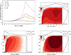 |
Fig. 1. Top left: Companion frequency for a primary mass of 20 M⊙ at different orbital periods. The blue line represents the companion frequency from Moe & Di Stefano (2017) for a 20 M⊙ primary, while the other colors show extrapolated companion frequencies for different minimum mass ratios (qmin). Top right: Initial orbital distribution of isolated binaries with a qmin = 0.001. Bottom panels: Initial inner and outer orbital distributions of triple systems with qmin = 0.001. |
2.4. Birth rate calculation
We used a method similar to that of Naoz et al. (2016), Shariat et al. (2025c) and Generozov & Perets (2024) to estimate the birth rate (R) of the dBH-LC population. Using the sampling described in Sect. 2.3, we performed 4 × 10⁵ triple simulations and 4 × 10⁶ binary simulations to reduce the uncertainty in the Rbirth rate calculation. Specifically, we used the following equation:
 (8)
(8)
where, M* is the average stellar mass calculated from the initial mass function of Kroupa (2001), with a value of ∼0.572 M⊙, which is consistent with the result from Hamers et al. (2022b). We note that fm1 > 8 ≅ 0.006 and fm1 > 18 ≅ 0.002 are the fraction of stars with masses greater than 8 M⊙ or 18 M⊙, based on the initial mass function from Kroupa (2001). Further, ftriple and fbinary represent the binary and triple fractions for massive stars, respectively. The probability of a triple is treated as a function of the primary mass, M1, based on the observational results of Moe & Di Stefano (2017). This probability depends on M1 as well as the likelihood of its companions forming at different orbital periods. In other words, ftriple and fbinary are obtained by convolving the initial mass function from Kroupa (2001) with the triple fraction, similar to the approach used in the study by Offner et al. (2023). Using this method, we obtained ftriple = 84% and fbinary = 13%. It is worth noting that these results are based on extrapolation down to a minimum mass ratio of qmin = 0.01. All of the above fractions are independent of the outcomes from our models. Only the overall fraction of systems that evolve into dBH-LCs (i.e., fdBH − LC) depends on the outcome of our population synthesis. It is important to emphasize that fdBH − LC is inevitably a function of the assumed initial mass and separation distributions, making it sensitive to model uncertainties.
3. Results
Using MOBSE and TSE, we evolved the initial massive binary and triple populations sampled in Sect. 2.3. In the following sections, we first present two examples of dBH-LCs formed through triple evolution. Then, we show a series of results for dBH-LCs formed through IBE and triple evolution.
3.1. Example channels for dBH-LC formation from triple systems
In the simulations of triple evolution, dBH-LCs are primarily formed through two channels: (1.) The inner binary undergoes a merger, and the merger product later evolves into a BH. In this case, it forms a dBH-LC with the original tertiary. (2.) One of the massive stars in the triple undergoes a SN. If the inner orbit remains bound after the SN but the outer orbit is disrupted, the remaining binary may evolve into a dBH-LC at a later stage.
In Fig. 2, we show two typical examples of dBH-LC formation. In the left panel, the triple experiences strong ZLK oscillations. Because the inner orbit is wide (about 1900 R⊙), the tidal effect is weak. As the primary evolves, it begins RLOF at periastron at ∼7.75 Myr. During the non-conservative MT process (gray area), the donor’s mass decreases from 22.5 M⊙ to 8.4 M⊙. The accretor’s mass increases from 14.9 M⊙ to 20.4 M⊙. About 8.6 M⊙ of mass is lost from the binary system. The inner eccentricity is reduced from 0.49 to 0.34. In the later evolution, the primary becomes a helium star. At 8.6 Myr, it undergoes a SN and forms a BH with a mass of 3.5 M⊙. After the SN, the outer orbit is disrupted, but the inner binary stays bound. At this point, a dBH-LC system is formed (red area), with an eccentricity of 0.3, a separation (orbital period) of 2332 R⊙ (2671 days), and masses of 3.5 M⊙ for the BH and 20.4 M⊙ for the LC.
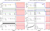 |
Fig. 2. Examples of dBH-LC formation through SN or inner binary merger in triple evolution are shown. Both panels display the evolution of component mass, radius, orbital separation, and eccentricity as functions of time. In both panels, the gray region indicates the phase when the inner binary undergoes RLOF, and the red region marks the dBH-LC phase. In addition, the initial parameters of the two triples shown in the figure are as follows: In the left panel, the masses of the system are m1 = 23.57 M⊙, m2 = 14.96 M⊙, and m3 = 0.13 M⊙. The semi-major axes and eccentricities are ain = 1902.10 R⊙, aout = 19130.05 R⊙, ein = 0.51, and eout = 0.46. The inclinations and arguments of pericenter are cos iin = 0.80, cos iout = 0.04, ωin = 6.00, and ωout = 0.07. In the right panel, the masses of the triple are m1 = 52.84 M⊙, m2 = 8.07 M⊙, and m3 = 9.00 M⊙. The semi-major axes and eccentricities are ain = 66.26 R⊙, aout = 2666.19 R⊙, ein = 0.18, and eout = 0.66. The inclinations and arguments of pericenter are cos iin = −0.98, cos iout = −0.99, ωin = 0.79, and ωout = 2.99. |
The right panel of Fig. 2 shows the inner binary merger (IBM) during the evolution of the triple. Later, the outer binary evolves and forms a dBH-LC. During the evolution, because the initial inner orbital separation is small (about 66 R⊙), the ZLK effect of the triple is strongly suppressed by tides, and the periodic oscillation of the inner eccentricity (ein) is very weak. The inverse of the spin period ( ) of each of the two stars in the inner binary is very short (∼0.43 days for the primary and ∼0.13 days for the secondary). This period is much shorter than the orbital period of the inner binary (∼8 days), and this causes the rotation angular momentum of the two stars in the inner binary to transfer to the inner orbit, which in turn causes ein and ain to increase. A similar conclusion was found in the analyses by Correia et al. (2011, 2016), and Zoppetti et al. (2019) and the analysis in Sect. 2.1.2 of Stegmann et al. (2022). At about 3.01 Myr, the primary undergoes RLOF while on the MS stage. Because the mass ratio is too small (q =
  = 0.167), a merger occurs. According to the assumption by Hurley et al. (2002), when two MS stars merge, their material mixes completely, and the merger product remains an MS star. At 7.97 Myr, the merger product undergoes MT with its companion (the original tertiary) during the Hertzsprung gap phase. Because the mass ratio was too small (q =
  = 0.196), this MT leads to a common envelope evolution (CEE). During the CEE, the post-merger binary survives, and the envelope of the primary is successfully ejected. It becomes a 17.2 M⊙ Wolf-Rayet star, and the orbital separation shrinks from 3421 R⊙ to 13 R⊙. Due to strong stellar winds during the Wolf-Rayet phase, it becomes a Wolf-Rayet star of about 10.6 M⊙ before undergoing SN. In the end, it forms a 6.4 M⊙ BH through complete fallback, and together with a 9 M⊙ LC (the original tertiary), it forms a dBH-LC system (red area).
3.2. Population synthesis results
In this section we first focus on the properties of all dBH-LCs and then narrow our focus to the dBH-LCs that are potentially observable by Gaia. We divided the dBH-LC population into dormant black-hole main sequence (dBH-MS) and dormant black-hole post main sequence (dBH-PMS) systems. The dBH-MSs are usually binaries that form just after the BH is born. For dBH-LCs formed through the IBE channel, we classify them into three sub-channels: no MT channel, indicating none of the stars in the binary or triple undergo MT before forming the dBH-LC; MT channel, in which case the stars experience only stable MT before forming the dBH-LC; and CE channel, where at least one episode of CEE occurs before the dBH-LC is formed. For triple evolution, as described in Sect. 3.1, we divided the formation channels into IBM and SN.
Figure 3 shows the birth rate distributions of dBH-MS and dBH-PMS formed through IBE and triple evolution. In Fig. 3, the birth rates of the parameter distributions of the dBH-MSs formed from triple evolution are one to two orders of magnitude higher than those formed from IBE. For MBH, the maximum MBH formed by IBE (∼25 M⊙) is about three times smaller than that formed by triple evolution (about 73 M⊙; see also Generozov & Perets 2024). In triple evolution, the MBH (> 25 M⊙) come from the IBM channel (see the analysis below for details). The MBH formed by the SN channel and the IBM channel both show an approximately monotonic decrease. For IBE, low-mass BHs (< 5 M⊙) mainly come from the CE channel. These BHs mainly form through accretion-induced collapse and core-collapse SN. When BHs with masses greater than 15 M⊙ form, the larger the MBH, the stronger the fallback (Fryer et al. 2012). When BHs form through full fallback, they experience very weak kicks. This increases the birth rate of dBH-MS with BHs larger than 15 M⊙. In addition, it allows for the formation of dBH-MS with BHs larger than 15 M⊙ in the long orbital period range (> 104.0 days). For MLCs, both triple evolution and IBE tend to form more massive LCs (> 10 M⊙). This is either because more massive LCs survive more easily in the CEE process or because they are more likely to remain bound in the SN process due to higher gravitational binding energy. For Porb and eccentricity (e), the dBH-MS formed by triple evolution and IBE both show traces of the initial outer binary distribution and the initial IBE distribution.
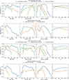 |
Fig. 3. At the metallicity of the MW, birth rate distributions of the physical parameters of dBH-MS and dBH-PMS formed through IBE and triple evolution. |
Considering that Gaia has a maximum observation duration of 10 years for dBH-LCs, we focused on dBH-LCs with Porb < 10 yr. Figures 4 and 5 present the 2D histograms of dBH-MS and dBH-PMS with Porb < 10 yr formed through IBE and triple evolution. The green crosses indicate the observational data from Table 1. Based on Figs. 4 and 5, we find that both IBE and triple evolution can basically explain the pairwise physical quantities of these observations. However, our model has difficulty explaining the MBH of Gaia BH3. This is model dependent and may vary significantly with the assumed metallicity, as Gaia BH3 is extremely metal poor. The birth rate of dBH-LCs in each bin from triple evolution is generally higher than that from the IBE model. This means that triple evolution has a greater advantage in explaining the currently observed dBH-LCs. However, we note that our triple evolution model is still insufficient for the statistical properties of dBH-LCs with Porb < 10 yr. This is because the outer orbital periods in our initial sampling of triples are mainly concentrated around 105 days. In triple evolution, the formation of dBH-LCs is mainly contributed by the IBM channel, and most of the dBH-LCs formed through this channel have Porb < 10 yr (see also Fig. 3). In addition, from comparison of Figs. 4 and 5, we find that some PMS stars may interact with the BH. This causes some low-mass BHs to merge with the PMS in the CEE process. It also causes the stable MT channel and the CE channel in dBH-PMS to produce more low-mass LCs (< 1 M⊙) and circularized dBH-PMS systems (e = 0). In addition, the mass-loss rate of PMS stars is usually higher than that of MS stars. This stronger mass-loss rate can drive orbital expansion, which causes the orbital periods of dBH-PMS to be generally higher than those of dBH-MS, such as Gaia BH1, Gaia BH2 and Gaia BH3.
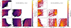 |
Fig. 4. Two-dimensional birth rate distribution of dBH-MS in the MW shown as a function of LC mass (MLC), BH mass (MBH), orbital period (Porb), and eccentricity (e). The color in each pixel is scaled according to the birth rate of dBH-LC binaries. Left panels: dBH-MS formed through IBE. Right panels: dBH-MS formed through triple evolution. The dark green crosses represent the observational data from Table 1. It is worth noting that our study focuses more on the differences between the dBH-LC populations formed through IBE and triple evolution. Therefore, in Table 1, we classify the observations only by the stellar types of the LCs. We emphasize that explaining these observations still requires attention to additional physical properties (e.g., the metallicity of each observation). |
Table 2 shows the birth rates of dBH-LCs formed by IBE and triple evolution in the MW. In the IBE model, the birth rate of dBH-LCs is 4.35 × 10⁻⁵ yr−1. This is similar to the result calculated by Shao & Li (2019, see their Table 1). In the triple evolution model, the birth rate of dBH-LCs is 1.47 × 10⁻³ yr−1. This is one or two orders of magnitude higher than the birth rate of dBH-LCs formed by IBE, which can be explained by two key factors: the higher triple fraction of massive stars (contributing at most one order of magnitude) and, more importantly, the effect of triple dynamics, which significantly enhances the birth rate of dBH-LCs through triple evolution. This result shows that the evolution of massive stars in triples is more likely to form dBH-LCs. This conclusion is similar to that of Generozov & Perets (2024). In addition, an LC in the PMS phase must have evolved through the MS phase. However, not all dBH-MS systems will later evolve into dBH-PMS systems. This is because, during PMS evolution, the LC in a dBH-MS system may interact with the BH – such as through CEE. These interactions may result in the formation of a BH X-ray binary or in a merger between the LC and BH (e.g., if the system does not survive CEE). As a result, in both the IBE model and the triple evolution model, the birth rate of dBH-MS is higher than that of dBH-PMS. Furthermore, estimating the number of dBH-LCs is timely regarding the upcoming Gaia DR4. In detail, we estimated the number by multiplying the birth rate with the average lifetime of LCs in different mass bins. Because the recently observed dBH-LCs are not far from us (e.g., Gaia BH1, Gaia BH2 and Gaia BH3 are at about 480 pc (El-Badry et al. 2023b), 1.16 kpc (El-Badry et al. 2023a), and 590 pc (Gaia Collaboration 2024) from the Sun), we calculated the birth rate and number of nearby dBH-LCs, as shown in Table 3. In this calculation, we assumed that dBH-LCs remain close to their birth locations and did not consider their possible motion. Our sampling method for the distance between a dBH-LC and the Sun is similar to that in Sect. 2.4 of He et al. (2024). There are only a few studies that estimate the total number of dBH-LCs through triple evolution. Most previous works focus on isolated binary evolution or dynamical evolution. Breivik et al. (2017), Chawla et al. (2022), Shao & Li (2019), Di Carlo et al. (2024), and Nagarajan et al. (2025) respectively predicted the number of observable dBH-LCs to be 3800–12 000, 30–300, 470–12 000, ∼155 724, and ∼19 466. These differences can be explained by different model assumptions and choices of observational effects. In Table 3, our binary evolution model predicts about 3000 dBH-LCs. This number is lower than most of the previous predictions. The difference comes from our lower initial binary fraction (13% in our work). Finally, by combining the binary evolution channel and the triple evolution channel, we estimate that the entire MW contains approximately 87 000 dBH-LCs with Porb < 10 yr. Among them, about 75 000 dBH-LCs are within 20 kpc from the Sun, and about 570 dBH-LCs are within 1 kpc.
Birth rates of dBH-LCs (including dBH-MS and dBH-PMS), dBH-MS, and dBH-PMS under different evolution models at the metallicity of the MW.
Birth rate and number (in parentheses) of dBH-LCs with an orbital period of Porb < 10 yr.
In addition, we note that triple evolution can produce dBH-LCs with more massive BHs than can be formed through IBE (e.g., MBH > 30 M⊙; see also Fig. 3). As analyzed for Fig. 3, these dBH-LCs with more massive BHs are formed through the IBM channel of triple evolution. In Fig. 6, we show an example of how a dBH-LC with a massive BH (> 60 M⊙) can form through triple evolution. In the triple evolution of Fig. 6, a primary with an initial mass of 78.41 M⊙ evolves first. The inner binary then undergoes strong ZLK oscillations, and its inner eccentricity shows long-term periodic changes between 0.25 and 0.78. As the radius of the primary expands, tidal effects gradually increase. When the precession caused by tides dominates over the precession caused by the ZLK mechanism, the inner binary can effectively decouple from the tertiary (Stegmann et al. 2022). This eventually suppresses any ZLK oscillations, reducing the periodic oscillations of the inner eccentricity (Toonen et al. 2016; Dorozsmai et al. 2024). The primary undergoes RLOF at about 3.63 Myr. As MT continues, the secondary in the inner binary also expands. At about 3.73 Myr, the primary evolves into an Hertzsprung gap star and comes into contact with the secondary (an MS star), leading to a merger. According to the collision matrix of Hurley et al. (2002); the 3D simulations of binary mergers by Glebbeek et al. (2013), Costa et al. (2022), and Costa et al. (2022); and the simulations of binary mergers and the evolution of merger products using the 1D stellar evolution code MESA by Renzo et al. (2020), Costa et al. (2022), and Costa et al. (2022), the secondary (MS star) dissolves in the envelope of the Hertzsprung gap star. This makes the merger product have a larger envelope mass and finally forms a merger product with a small helium core mass (about 24.71 M⊙) but a large envelope mass (about 88.05 M⊙). This merger product undergoes significant mass loss in the later evolution. However, before the SN, it still has about 35.3 M⊙ of envelope mass. This causes a large fallback during the SN, with a negligible natal kick. Finally, it forms a dBH-LC composed of a 64.74 M⊙ BH and a 2.79 M⊙ MS star (the original tertiary). Therefore, through triple evolution, BH binaries where BH mass lies in the PISN range (about 60 M⊙ ∼ 120 M⊙) can be produced. We also calculated that the birth rate of dBH-LCs with a BH in the PISN range formed in this way at thin disk metallicity is about 1.78 × 10⁻⁶ yr−1.
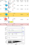 |
Fig. 6. Example of a dBH-LC with a BH in the PISN range formed through triple evolution. In the upper panel, the yellow area and the red area represent the formation of the post-merger binary and the formation of the dBH-LC, respectively. In the lower panel, the gray area represents the phase when the inner binary undergoes MT. |
In Fig. 7, we present the 2D histogram of dBH-LC systems formed through the IBM channel in triple evolution. In Fig. 7, dBH-LCs with MBH values greater than 30 M⊙ generally have very long orbital periods (Porb > 104 days) that are much longer than the observation duration of Gaia. Compared to Gaia’s maximum observational baseline (10 years), the maximum BH masses for which Gaia can at most fully resolve the orbit, resolve half of the orbit, and resolve one-third of the orbit are approximately 25 M⊙, 30 M⊙, and 40 M⊙, respectively. This is because the merger products of the progenitor stars that form these massive BHs have very high masses. Their strong stellar winds can expand the orbital periods of the post-merger binaries so that they become very large. In addition, dBH-LC systems formed through the IBM channel show a gap in orbital periods between ∼102 and 103 days. The main reason for this gap is that, in the IBM channel, the merger product and its LC either undergo CEE and form a short-period system, or they never interact and form a long-period system. This result is very similar to the findings of Nagarajan et al. (2025, see their Fig. 1).
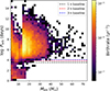 |
Fig. 7. Two-dimensional birth rate distribution of MBH − Porb for dBH-MS formed through the IBM channel in triple evolution. This figure also shows one times, two times, and three times Gaia’s maximum observational baseline (10 years), which correspond to the cases where Gaia can at most fully resolve the entire orbit, half of the orbit, and one-third of the orbit, respectively. |
4. Discussion
As discussed in Sect. 3, although we have considered the formation of dBH-LC populations under different evolutionary models, metallicities, and formation channels, the evolution of massive stars is highly complex. Therefore, our conclusions still carry uncertainties. As in the recent work by Sciarini et al. (2025), our study is based on the rapid stellar evolution (RSE) code that uses the fitting formulas from Hurley et al. (2000, 2002). However, this approach still shows significant differences from detailed stellar evolution codes (e.g., MESA code; Paxton et al. 2011, 2013, 2015, 2018, 2019) in modeling the evolution of massive stars. Typically, these fitting formulas do not self-consistently account for the effects of mass loss on stellar evolution (Bavera et al. 2023). As pointed out in the works of Sciarini et al. (2025) and Shariat et al. (2025c), compared to the MESA code, the SSE code tends to overestimate the radii of massive stars and their stellar winds. These differences can lead to significant discrepancies in the predicted final outcomes and orbital evolution of massive stars. For example, the RSE code may result in an overestimation of the interaction frequency among massive stars, affect the efficiency of tidal interactions, and underestimate the effectiveness of the ZLK mechanism in triple evolution. In addition, the TSE code currently does not model systems undergoing dynamical instability or RLOF involving the tertiary. In the study by Glanz & Perets (2021), Hamers et al. (2022a,b), Li et al. (2025b), Bruenech et al. (2025) and Kummer et al. (2025b) it was shown that MT from the tertiary to the inner binary or dynamical instability in triple systems can lead to inner binary mergers or the ejection of the lowest-mass star. The contribution of such scenarios to the dBH-LC population remains unknown.
For the BH SN kicks, we adopted the more recent prescription proposed by Giacobbo & Mapelli (2020). This SN model can explain a wide range of observational constraints, including the merger rates of binary neutron stars, binary BHs, and neutron star-BH binaries inferred by the LIGO-Virgo collaboration (e.g., GW170817; Abbott et al. 2019); the natal kicks of young pulsars; and the differences in kick between core-collapse SNe, electron-capture SNe, and ultra-stripped SNe in binary systems. Specifically, this SN prescription accounts for the remnant mass, the fallback fraction, and the ejecta mass (see Eq. (4)). According to this model, the natal kick distribution of BHs shows two peaks: one at ∼0 km/s (corresponding to BHs formed via direct collapse, which make up about 60% of the population), and another at tens of kilometers per second (≤100 km/s). The average natal kick velocity for BHs under this prescription is ∼30 km/s (see Table 2 in Giacobbo & Mapelli 2020). At present, the distribution of BH natal kicks is still not well understood. Recent studies support the idea that many BHs receive negligible natal kicks at birth (Mirabel & Rodrigues 2003; Shenar et al. 2022; Burdge et al. 2024; Vigna-Gómez et al. 2024; van Son et al. 2025; Nagarajan & El-Badry 2025; Shariat et al. 2025c). In particular, Burdge et al. (2024) and Shariat et al. (2025c) found that known BHs in a triple likely formed without any significant kicks. However, some BHs do appear to receive relatively large natal kicks, ranging from tens to over one hundred kilometers per second (Andrews & Kalogera 2022; Kimball et al. 2023; Mata Sánchez et al. 2025). In addition, previous studies have shown that low natal kicks (< 40 ∼ 50 km/s) are generally favored for the formation of wide-orbit BH binaries (e.g., Gaia BH1/2/3; El-Badry et al. 2023b,a; Kotko et al. 2024; Li et al. 2024b).
Due to observational limitations, the statistics of binaries or multiple systems with low mass ratios remain highly uncertain, mainly because of the large brightness contrast. In this work, we extrapolated the minimum companion mass down to the brown dwarf boundary, assuming a hydrogen-burning limit of 0.08 M⊙. Our extrapolated results are consistent with those of Generozov & Perets (2024), who also found that lowering the minimum mass ratio leads to a significantly increased probability of forming companions at wider separations (with a typical peak orbital period around 105.5 days; see also Fig. 1). This suggests that the primary is very likely to host one or more companions in wide orbits (i.e., to form in binary or multiple systems), but such companions are extremely difficult to detect observationally, which introduces large uncertainties in the statistics of low mass-ratio companions. On the other hand, our study is limited to systems with up to triple systems. In reality, the probability of forming higher-order multiples increases significantly with the mass of the primary (see also Fig. 39 in Moe & Di Stefano 2017). This implies that the binary and triple fractions used in our convolution also carry uncertainties.
This study is limited by the assumption of a single metallicity value (Z = Z⊙ = 0.014) to represent that of the MW. In reality, the thick disk of the MW is characterized by a lower metallicity, typically Z = 0.15 Z⊙ (Yoshii 2013). It is well known that as metallicity decreases, the opacity of massive stars is reduced, leading to lower mass-loss rates and smaller maximum radii (Vink et al. 2001). Consequently, orbital expansion in a binary or triple is expected to be suppressed for low metallicity populations, and the probability of binary interactions is reduced. More importantly, massive stars with a lower metallicity tend to form more massive BHs, which is crucial for predicting a dBH-LC with a heavy BH (e.g., Gaia BH3). Additionally, the reduced mass-loss rate in low metallicity environments allows massive stars to retain more of their rotational angular momentum during evolution. This allows rotationally induced mixing to drive chemically homogeneous evolution (CHE) in massive stars (Zahn 1975; Hut 1981; Packet 1981; Maeder 1987; Pols et al. 1991; Podsiadlowski et al. 1992; Petrovic et al. 2005; Yoon & Langer 2005; Yoon et al. 2006; de Mink et al. 2009; Tylenda et al. 2011; Brott et al. 2011; Vanbeveren et al. 2013; Shao & Li 2014; Köhler et al. 2015; Szécsi et al. 2015; Renzo & Götberg 2021; Li et al. 2023). Notably, CHE is a key pathway for forming Wolf-Rayet stars (Cui et al. 2018; Lu et al. 2023; Li et al. 2024a; He et al. 2025), BHs (Mandel & de Mink 2016; Marchant et al. 2016; de Mink & Mandel 2016; Hastings et al. 2020; du Buisson et al. 2020; Riley et al. 2021; Li et al. 2025a), magnetars, and the progenitors of long gamma-ray bursts (Podsiadlowski et al. 2004; Yoon & Langer 2005; Yoon et al. 2006; Woosley & Heger 2006; Martins et al. 2013). In particular, Dorozsmai et al. (2024) showed that in a triple, the inner binary can undergo CHE and produce double BHs, which may eventually merge due to a ZLK mechanism within the triple. This channel may also be important for the formation of dBH-LC.
5. Conclusions
In this study, we have used the MOBSE and TSE codes to simulate the formation and evolution of dBH-LCs in the MW. We considered progenitor systems originating from both isolated binaries and hierarchical triples. In the MW, the birth rates of dBH-LC systems calculated from the IBE and triple evolution channels are 4.35 × 10⁻⁵ yr−1 and 1.47 × 10⁻³ yr−1, respectively. Compared to isolated binaries, massive stars in triples are more likely to interact within the inner binary due to ZLK oscillations. As a result, dBH-LC systems are predominantly formed through the channel in which the inner binary merges and forms a new binary (see Fig. 3). In our calculation, the birth rate of dBH-LCs from triple evolution is one to two orders of magnitude higher than that from the IBE channel. In addition, we find that the dBH-LC formed from post-merger binaries in triple systems have a much larger MBH than those formed through the IBE channel. The reason is that the merger product of a MS plus CHeB inner binary is a massive star with a small helium core and a large envelope. Because the helium core is small and the total mass is large, these merger products can form BHs in the predicted PISN range (60 M⊙ ∼ 120 M⊙).
We summarize the main results on the orbital properties of dBH-MS and dBH-PMS formed in the MW as follows. (1.) For dBH-MS, the MLC from the IBE channel shows two peaks in the range of 10–63 M⊙. The low-mass LCs are mainly contributed by the no MT channel. At the same time, the eccentricities of dBH-MS from the IBE channel cover a wide range. The circularized dBH-MS are mainly contributed by the CE and stable MT channels. On the other hand, the MLC of dBH-MS formed through triple evolution shows peaks at 1 M⊙ and 63 M⊙, mainly contributed by the IBM and SN channels, respectively. (2.) For dBH-PMS, because some LCs undergo MT with the BH during later evolution, both the IBE and triple evolution channels produce more low-mass companions (MLC < 1.6 M⊙) and circularized systems compared to dBH-MS.
Our results show that triple evolution plays a key role in the formation of dBH-LCs and helps explain observational phenomena that the IBE model struggles to account for. This highlights the importance of considering triple evolution in future studies to better understand the diversity of dBH-LC systems.
Acknowledgments
This work received the support of the National Natural Science Foundation of China under grants 12373038, 12563007, U2031204, and 12288102; the Natural Science Foundation of Xinjiang No. 2022TSYCLJ0006 and 2022D01D85; the China Manned Space Program grant No. CMS-CSST-2025-A15. AP23490322 – Exploration of Thermodynamic Properties of Relativistic Compact Objects Within the Framework of Geometrothermodynamics (GTD), Grant financing for scientific and/or scientific-technical projects for 2024–2026, Ministry of Science and Higher Education of the Republic of Kazakhstan.
References
- Abbott, B. P., Abbott, R., Abbott, T. D., et al. 2019, ApJ, 882, L24 [Google Scholar]
- Anderson, K. R., Storch, N. I., & Lai, D. 2016, MNRAS, 456, 3671 [NASA ADS] [CrossRef] [Google Scholar]
- Andrews, J. J., & Kalogera, V. 2022, ApJ, 930, 159 [NASA ADS] [CrossRef] [Google Scholar]
- Andrews, J. J., Taggart, K., & Foley, R. 2022, arXiv e-prints [arXiv:2207.00680] [Google Scholar]
- Antonini, F., Murray, N., & Mikkola, S. 2014, ApJ, 781, 45 [NASA ADS] [CrossRef] [Google Scholar]
- Antonini, F., Chatterjee, S., Rodriguez, C. L., et al. 2016, ApJ, 816, 65 [NASA ADS] [CrossRef] [Google Scholar]
- Antonini, F., Toonen, S., & Hamers, A. S. 2017, ApJ, 841, 77 [NASA ADS] [CrossRef] [Google Scholar]
- Barkat, Z., Rakavy, G., & Sack, N. 1967, Phys. Rev. Lett., 18, 379 [Google Scholar]
- Bartos, I., Rosswog, S., Gayathri, V., et al. 2023, arXiv e-prints [arXiv:2302.10350] [Google Scholar]
- Bataille, M., Libert, A.-S., & Correia, A. C. M. 2018, MNRAS, 479, 4749 [NASA ADS] [CrossRef] [Google Scholar]
- Bavera, S. S., Fragos, T., Zapartas, E., et al. 2023, Nat. Astron., 7, 1090 [NASA ADS] [CrossRef] [Google Scholar]
- Belczynski, K., Kalogera, V., Rasio, F. A., et al. 2008, ApJS, 174, 223 [Google Scholar]
- Bodensteiner, J., Shenar, T., Mahy, L., et al. 2020, A&A, 641, A43 [NASA ADS] [CrossRef] [EDP Sciences] [Google Scholar]
- Bond, J. R., Arnett, W. D., & Carr, B. J. 1984, ApJ, 280, 825 [NASA ADS] [CrossRef] [Google Scholar]
- Breivik, K., Chatterjee, S., & Larson, S. L. 2017, ApJ, 850, L13 [CrossRef] [Google Scholar]
- Brott, I., de Mink, S. E., Cantiello, M., et al. 2011, A&A, 530, A115 [NASA ADS] [CrossRef] [EDP Sciences] [Google Scholar]
- Brown, G. E., & Bethe, H. A. 1994, ApJ, 423, 659 [NASA ADS] [CrossRef] [Google Scholar]
- Bruenech, C. W., Boekholt, T., Kummer, F., & Toonen, S. 2025, A&A, 693, A14 [NASA ADS] [CrossRef] [EDP Sciences] [Google Scholar]
- Burdge, K. B., El-Badry, K., Kara, E., et al. 2024, Nature, 635, 316 [NASA ADS] [CrossRef] [Google Scholar]
- Casares, J., Negueruela, I., Ribó, M., et al. 2014, Nature, 505, 378 [Google Scholar]
- Chakrabarti, S., Simon, J. D., Craig, P. A., et al. 2023, AJ, 166, 6 [NASA ADS] [CrossRef] [Google Scholar]
- Chawla, C., Chatterjee, S., Breivik, K., et al. 2022, ApJ, 931, 107 [NASA ADS] [CrossRef] [Google Scholar]
- Chawla, C., Chatterjee, S., Shah, N., & Breivik, K. 2024, ApJ, 975, 163 [NASA ADS] [Google Scholar]
- Chen, K.-J., Woosley, S., Heger, A., Almgren, A., & Whalen, D. J. 2014, ApJ, 792, 28 [NASA ADS] [CrossRef] [Google Scholar]
- Chomiuk, L., & Povich, M. S. 2011, AJ, 142, 197 [Google Scholar]
- Claeys, J. S. W., Pols, O. R., Izzard, R. G., Vink, J., & Verbunt, F. W. M. 2014, A&A, 563, A83 [NASA ADS] [CrossRef] [EDP Sciences] [Google Scholar]
- Corral-Santana, J. M., Casares, J., Muñoz-Darias, T., et al. 2016, A&A, 587, A61 [NASA ADS] [CrossRef] [EDP Sciences] [Google Scholar]
- Correia, A. C. M., Laskar, J., Farago, F., & Boué, G. 2011, Celest. Mech. Dyn. Astron., 111, 105 [NASA ADS] [CrossRef] [Google Scholar]
- Correia, A. C. M., Boué, G., & Laskar, J. 2016, Celest. Mech. Dyn. Astron., 126, 189 [NASA ADS] [CrossRef] [Google Scholar]
- Costa, G., Ballone, A., Mapelli, M., & Bressan, A. 2022, MNRAS, 516, 1072 [NASA ADS] [CrossRef] [Google Scholar]
- Costa, G., Chruślińska, M., Klencki, J., et al. 2023, arXiv e-prints [arXiv:2311.15778] [Google Scholar]
- Crowther, P. A., Broos, P. S., Townsley, L. K., et al. 2022, MNRAS, 515, 4130 [NASA ADS] [CrossRef] [Google Scholar]
- Cui, Z., Wang, Z., Zhu, C., et al. 2018, PASP, 130, 084202 [NASA ADS] [CrossRef] [Google Scholar]
- de Mink, S. E., & Mandel, I. 2016, MNRAS, 460, 3545 [NASA ADS] [CrossRef] [Google Scholar]
- de Mink, S. E., Cantiello, M., Langer, N., et al. 2009, A&A, 497, 243 [NASA ADS] [CrossRef] [EDP Sciences] [Google Scholar]
- Di Carlo, U. N., Agrawal, P., Rodriguez, C. L., & Breivik, K. 2024, ApJ, 965, 22 [CrossRef] [Google Scholar]
- Dorozsmai, A., Toonen, S., Vigna-Gómez, A., de Mink, S. E., & Kummer, F. 2024, MNRAS, 527, 9782 [Google Scholar]
- du Buisson, L., Marchant, P., Podsiadlowski, P., et al. 2020, MNRAS, 499, 5941 [Google Scholar]
- Duquennoy, A., & Mayor, M. 1991, A&A, 248, 485 [NASA ADS] [Google Scholar]
- El-Badry, K., Rix, H.-W., Cendes, Y., et al. 2023a, MNRAS, 521, 4323 [NASA ADS] [CrossRef] [Google Scholar]
- El-Badry, K., Rix, H.-W., Quataert, E., et al. 2023b, MNRAS, 518, 1057 [Google Scholar]
- Ford, E. B., Kozinsky, B., & Rasio, F. A. 2000, ApJ, 535, 385 [NASA ADS] [CrossRef] [Google Scholar]
- Fragione, G., Loeb, A., & Rasio, F. A. 2020a, ApJ, 895, L15 [NASA ADS] [CrossRef] [Google Scholar]
- Fragione, G., Martinez, M. A. S., Kremer, K., et al. 2020b, ApJ, 900, 16 [NASA ADS] [CrossRef] [Google Scholar]
- Fryer, C. L., Belczynski, K., Wiktorowicz, G., et al. 2012, ApJ, 749, 91 [Google Scholar]
- Gaia Collaboration (Panuzzo, P., et al.) 2024, A&A, 686, L2 [NASA ADS] [CrossRef] [EDP Sciences] [Google Scholar]
- Generozov, A., & Perets, H. B. 2024, ApJ, 964, 83 [NASA ADS] [CrossRef] [Google Scholar]
- Giacobbo, N., & Mapelli, M. 2020, ApJ, 891, 141 [NASA ADS] [CrossRef] [Google Scholar]
- Giacobbo, N., Mapelli, M., & Spera, M. 2018, MNRAS, 474, 2959 [Google Scholar]
- Giesers, B., Dreizler, S., Husser, T.-O., et al. 2018, MNRAS, 475, L15 [NASA ADS] [CrossRef] [Google Scholar]
- Giesers, B., Kamann, S., Dreizler, S., et al. 2019, A&A, 632, A3 [NASA ADS] [CrossRef] [EDP Sciences] [Google Scholar]
- Glanz, H., & Perets, H. B. 2021, MNRAS, 500, 1921 [Google Scholar]
- Glebbeek, E., Gaburov, E., Portegies Zwart, S., & Pols, O. R. 2013, MNRAS, 434, 3497 [NASA ADS] [CrossRef] [Google Scholar]
- Hamers, A. S., Glanz, H., & Neunteufel, P. 2022a, ApJS, 259, 25 [NASA ADS] [CrossRef] [Google Scholar]
- Hamers, A. S., Perets, H. B., Thompson, T. A., & Neunteufel, P. 2022b, ApJ, 925, 178 [NASA ADS] [CrossRef] [Google Scholar]
- Hastings, B., Langer, N., & Koenigsberger, G. 2020, A&A, 641, A86 [EDP Sciences] [Google Scholar]
- He, J.-G., Shao, Y., Xu, X.-J., & Li, X.-D. 2024, MNRAS, 529, 1886 [Google Scholar]
- He, X., Lü, G., Zhu, C., et al. 2025, Res. Astron. Astrophys., 25, 035002 [Google Scholar]
- Heger, A., Fryer, C. L., Woosley, S. E., Langer, N., & Hartmann, D. H. 2003, ApJ, 591, 288 [CrossRef] [Google Scholar]
- Hobbs, G., Lorimer, D. R., Lyne, A. G., & Kramer, M. 2005, MNRAS, 360, 974 [Google Scholar]
- Hurley, J. R., Pols, O. R., & Tout, C. A. 2000, MNRAS, 315, 543 [Google Scholar]
- Hurley, J. R., Tout, C. A., & Pols, O. R. 2002, MNRAS, 329, 897 [Google Scholar]
- Hut, P. 1981, A&A, 99, 126 [NASA ADS] [Google Scholar]
- Iorio, G., Torniamenti, S., Mapelli, M., et al. 2024, A&A, 690, A144 [NASA ADS] [CrossRef] [EDP Sciences] [Google Scholar]
- Jayasinghe, T., Stanek, K. Z., Thompson, T. A., et al. 2021, MNRAS, 504, 2577 [NASA ADS] [CrossRef] [Google Scholar]
- Khokhlov, S. A., Miroshnichenko, A. S., Zharikov, S. V., et al. 2018, ApJ, 856, 158 [NASA ADS] [CrossRef] [Google Scholar]
- Kimball, C., Imperato, S., Kalogera, V., et al. 2023, ApJ, 952, L34 [Google Scholar]
- Köhler, K., Langer, N., de Koter, A., et al. 2015, A&A, 573, A71 [NASA ADS] [CrossRef] [EDP Sciences] [Google Scholar]
- Kotko, I., Banerjee, S., & Belczynski, K. 2024, MNRAS, 535, 3577 [Google Scholar]
- Kozai, Y. 1962, AJ, 67, 591 [Google Scholar]
- Kroupa, P. 2001, MNRAS, 322, 231 [NASA ADS] [CrossRef] [Google Scholar]
- Kruckow, M. U., Andrews, J. J., Fragos, T., et al. 2024, A&A, 692, A141 [NASA ADS] [CrossRef] [EDP Sciences] [Google Scholar]
- Kummer, F., Toonen, S., & de Koter, A. 2023, A&A, 678, A60 [NASA ADS] [CrossRef] [EDP Sciences] [Google Scholar]
- Kummer, F., Simion, G., Toonen, S., & de Koter, A. 2025a, A&A, 703, A123 [NASA ADS] [CrossRef] [EDP Sciences] [Google Scholar]
- Kummer, F., Toonen, S., Dorozsmai, A., Grishin, E., & de Koter, A. 2025b, A&A, 693, A84 [NASA ADS] [CrossRef] [EDP Sciences] [Google Scholar]
- Lennon, D. J., Dufton, P. L., Villaseñor, J. I., et al. 2022, A&A, 665, A180 [NASA ADS] [CrossRef] [EDP Sciences] [Google Scholar]
- Li, L., Zhu, C., Guo, S., Liu, H., & Lü, G. 2023, ApJ, 952, 79 [Google Scholar]
- Li, Z., Zhu, C., Lü, G., et al. 2024a, ApJ, 969, 160 [NASA ADS] [CrossRef] [Google Scholar]
- Li, Z., Zhu, C., Lu, X., et al. 2024b, ApJ, 975, L8 [NASA ADS] [CrossRef] [Google Scholar]
- Li, L., Lü, G., Zhu, C., et al. 2025a, Phys. Rev. D, 112, 103005 [Google Scholar]
- Li, Z., Lu, X., Lü, G., et al. 2025b, ApJ, 979, L37 [Google Scholar]
- Lidov, M. L. 1962, Planet. Space Sci., 9, 719 [Google Scholar]
- Liu, B., Lai, D., & Wang, Y.-H. 2019a, ApJ, 881, 41 [NASA ADS] [CrossRef] [Google Scholar]
- Liu, J., Zhang, H., Howard, A. W., et al. 2019b, Nature, 575, 618 [Google Scholar]
- Lu, X., Zhu, C., Liu, H., et al. 2023, A&A, 674, A216 [NASA ADS] [CrossRef] [EDP Sciences] [Google Scholar]
- Maeder, A. 1987, A&A, 178, 159 [NASA ADS] [Google Scholar]
- Mahy, L., Sana, H., Shenar, T., et al. 2022, A&A, 664, A159 [NASA ADS] [CrossRef] [EDP Sciences] [Google Scholar]
- Malkov, O. 2023, Galaxies, 11, 98 [Google Scholar]
- Mandel, I., & de Mink, S. E. 2016, MNRAS, 458, 2634 [NASA ADS] [CrossRef] [Google Scholar]
- Marchant, P., Langer, N., Podsiadlowski, P., Tauris, T. M., & Moriya, T. J. 2016, A&A, 588, A50 [NASA ADS] [CrossRef] [EDP Sciences] [Google Scholar]
- Mardling, R. A., & Aarseth, S. J. 2001, MNRAS, 321, 398 [NASA ADS] [CrossRef] [Google Scholar]
- Marín Pina, D., Rastello, S., Gieles, M., et al. 2024, A&A, 688, L2 [NASA ADS] [CrossRef] [EDP Sciences] [Google Scholar]
- Martinez, M. A. S., Fragione, G., Kremer, K., et al. 2020, ApJ, 903, 67 [Google Scholar]
- Martins, F., Depagne, E., Russeil, D., & Mahy, L. 2013, A&A, 554, A23 [NASA ADS] [CrossRef] [EDP Sciences] [Google Scholar]
- Mata Sánchez, D., Torres, M. A. P., Casares, J., et al. 2025, A&A, 693, A129 [Google Scholar]
- McClintock, J. E., & Remillard, R. A. 2006, in Compact stellar X-ray sources, eds. W. H. G. Lewin, & M. van der Klis, 39, 157 [NASA ADS] [CrossRef] [Google Scholar]
- Mirabel, I. F., & Rodrigues, I. 2003, Science, 300, 1119 [Google Scholar]
- Moe, M., & Di Stefano, R. 2017, ApJS, 230, 15 [Google Scholar]
- Nagarajan, P., & El-Badry, K. 2025, PASP, 137, 034203 [Google Scholar]
- Nagarajan, P., El-Badry, K., Chawla, C., et al. 2025, PASP, 137, 044202 [Google Scholar]
- Naoz, S. 2016, ARA&A, 54, 441 [Google Scholar]
- Naoz, S., & Fabrycky, D. C. 2014, ApJ, 793, 137 [Google Scholar]
- Naoz, S., Farr, W. M., Lithwick, Y., Rasio, F. A., & Teyssandier, J. 2013, MNRAS, 431, 2155 [NASA ADS] [CrossRef] [Google Scholar]
- Naoz, S., Fragos, T., Geller, A., Stephan, A. P., & Rasio, F. A. 2016, ApJ, 822, L24 [NASA ADS] [CrossRef] [Google Scholar]
- Naoz, S., Haiman, Z., Quataert, E., & Holzknecht, L. 2025, ApJ, 992, L12 [Google Scholar]
- Ober, W. W., El Eid, M. F., & Fricke, K. J. 1983, A&A, 119, 61 [NASA ADS] [Google Scholar]
- Offner, S. S. R., Moe, M., Kratter, K. M., et al. 2023, ASP Conf. Ser., 534, 275 [NASA ADS] [Google Scholar]
- Packet, W. 1981, A&A, 102, 17 [NASA ADS] [Google Scholar]
- Paxton, B., Bildsten, L., Dotter, A., et al. 2011, ApJS, 192, 3 [Google Scholar]
- Paxton, B., Cantiello, M., Arras, P., et al. 2013, ApJS, 208, 4 [Google Scholar]
- Paxton, B., Marchant, P., Schwab, J., et al. 2015, ApJS, 220, 15 [Google Scholar]
- Paxton, B., Schwab, J., Bauer, E. B., et al. 2018, ApJS, 234, 34 [NASA ADS] [CrossRef] [Google Scholar]
- Paxton, B., Smolec, R., Schwab, J., et al. 2019, ApJS, 243, 10 [Google Scholar]
- Perets, H. B., & Fabrycky, D. C. 2009, ApJ, 697, 1048 [Google Scholar]
- Petrovic, J., Langer, N., & van der Hucht, K. A. 2005, A&A, 435, 1013 [NASA ADS] [CrossRef] [EDP Sciences] [Google Scholar]
- Podsiadlowski, P., Joss, P. C., & Hsu, J. J. L. 1992, ApJ, 391, 246 [Google Scholar]
- Podsiadlowski, P., Mazzali, P. A., Nomoto, K., Lazzati, D., & Cappellaro, E. 2004, ApJ, 607, L17 [NASA ADS] [CrossRef] [Google Scholar]
- Pols, O. R., Cote, J., Waters, L. B. F. M., & Heise, J. 1991, A&A, 241, 419 [NASA ADS] [Google Scholar]
- Qian, S. B., Liao, W. P., & Fernández Lajús, E. 2008, ApJ, 687, 466 [NASA ADS] [CrossRef] [Google Scholar]
- Rajamuthukumar, A. S., Hamers, A. S., Neunteufel, P., Pakmor, R., & de Mink, S. E. 2023, ApJ, 950, 9 [CrossRef] [Google Scholar]
- Ramírez-Agudelo, O. H., Simón-Díaz, S., Sana, H., et al. 2013, A&A, 560, A29 [NASA ADS] [CrossRef] [EDP Sciences] [Google Scholar]
- Rastello, S., Iorio, G., Mapelli, M., et al. 2023, MNRAS, 526, 740 [NASA ADS] [CrossRef] [Google Scholar]
- Regály, Z., Fröhlich, V., & Vinkó, J. 2025, ApJ, 988, L7 [Google Scholar]
- Remillard, R. A., & McClintock, J. E. 2006, ARA&A, 44, 49 [Google Scholar]
- Renzo, M., & Götberg, Y. 2021, ApJ, 923, 277 [NASA ADS] [CrossRef] [Google Scholar]
- Renzo, M., Cantiello, M., Metzger, B. D., & Jiang, Y. F. 2020, ApJ, 904, L13 [NASA ADS] [CrossRef] [Google Scholar]
- Riley, J., Mandel, I., Marchant, P., et al. 2021, MNRAS, 505, 663 [Google Scholar]
- Rivinius, T., Baade, D., Hadrava, P., Heida, M., & Klement, R. 2020, A&A, 637, L3 [NASA ADS] [CrossRef] [EDP Sciences] [Google Scholar]
- Robin, A. C., Reylé, C., Derrière, S., & Picaud, S. 2003, A&A, 409, 523 [NASA ADS] [CrossRef] [EDP Sciences] [Google Scholar]
- Rodriguez, A. C., Cendes, Y., El-Badry, K., & Berger, E. 2023, arXiv e-prints [arXiv:2311.05685] [Google Scholar]
- Sahu, K. C., Anderson, J., Casertano, S., et al. 2025, ApJ, 983, 104 [Google Scholar]
- Salas, J. M., Naoz, S., Morris, M. R., & Stephan, A. P. 2019, MNRAS, 487, 3029 [Google Scholar]
- Saracino, S., Kamann, S., Guarcello, M. G., et al. 2022, MNRAS, 511, 2914 [NASA ADS] [CrossRef] [Google Scholar]
- Sciarini, L., Ekström, S., Kummer, F., et al. 2025, A&A, 698, A240 [NASA ADS] [CrossRef] [EDP Sciences] [Google Scholar]
- Sen, K., El Mellah, I., Langer, N., et al. 2024, A&A, 690, A256 [NASA ADS] [CrossRef] [EDP Sciences] [Google Scholar]
- Sen, K., Olejak, A., & Banerjee, S. 2025, A&A, 696, A54 [NASA ADS] [CrossRef] [EDP Sciences] [Google Scholar]
- Shao, Y., & Li, X.-D. 2014, ApJ, 796, 37 [Google Scholar]
- Shao, Y., & Li, X.-D. 2019, ApJ, 885, 151 [NASA ADS] [CrossRef] [Google Scholar]
- Shao, Y., & Li, X.-D. 2020, ApJ, 898, 143 [NASA ADS] [CrossRef] [Google Scholar]
- Shao, Y., & Li, X.-D. 2021, ApJ, 920, 81 [NASA ADS] [CrossRef] [Google Scholar]
- Shariat, C., Naoz, S., Hansen, B. M. S., et al. 2023, ApJ, 955, L14 [Google Scholar]
- Shariat, C., El-Badry, K., & Naoz, S. 2025a, PASP, 137, 094201 [Google Scholar]
- Shariat, C., El-Badry, K., Naoz, S., Rodriguez, A. C., & van Roestel, J. 2025b, PASP, 137, 074201 [Google Scholar]
- Shariat, C., Naoz, S., El-Badry, K., et al. 2025c, ApJ, 983, 115 [Google Scholar]
- Shariat, C., Naoz, S., El-Badry, K., et al. 2025d, ApJ, 978, 47 [Google Scholar]
- Shenar, T., Sana, H., Mahy, L., et al. 2022, Nat. Astron., 6, 1085 [NASA ADS] [CrossRef] [Google Scholar]
- Stegmann, J., & Antonini, F. 2024, J. Open Source Softw., 9, 7102 [Google Scholar]
- Stegmann, J., & Klencki, J. 2025, ApJ, 991, L54 [Google Scholar]
- Stegmann, J., Antonini, F., & Moe, M. 2022, MNRAS, 516, 1406 [NASA ADS] [CrossRef] [Google Scholar]
- Stephan, A. P., Naoz, S., Ghez, A. M., et al. 2016, MNRAS, 460, 3494 [NASA ADS] [CrossRef] [Google Scholar]
- Szécsi, D., Langer, N., Yoon, S.-C., et al. 2015, A&A, 581, A15 [NASA ADS] [CrossRef] [EDP Sciences] [Google Scholar]
- Tanikawa, A., Hattori, K., Kawanaka, N., et al. 2023, ApJ, 946, 79 [CrossRef] [Google Scholar]
- Thompson, T. A., Kochanek, C. S., Stanek, K. Z., et al. 2019, Science, 366, 637 [NASA ADS] [CrossRef] [Google Scholar]
- Timmes, F. X., Woosley, S. E., & Weaver, T. A. 1996, ApJ, 457, 834 [NASA ADS] [CrossRef] [Google Scholar]
- Toonen, S., Hamers, A., & Portegies Zwart, S. 2016, Comput. Astrophys. Cosmol., 3, 6 [NASA ADS] [CrossRef] [Google Scholar]
- Toonen, S., Perets, H. B., & Hamers, A. S. 2018, A&A, 610, A22 [NASA ADS] [CrossRef] [EDP Sciences] [Google Scholar]
- Toonen, S., Portegies Zwart, S., Hamers, A. S., & Bandopadhyay, D. 2020, A&A, 640, A16 [NASA ADS] [CrossRef] [EDP Sciences] [Google Scholar]
- Tylenda, R., Hajduk, M., Kamiński, T., et al. 2011, A&A, 528, A114 [NASA ADS] [CrossRef] [EDP Sciences] [Google Scholar]
- van Son, L. A. C., Roy, S. K., Mandel, I., et al. 2025, ApJ, 979, 209 [Google Scholar]
- Vanbeveren, D., Mennekens, N., Van Rensbergen, W., & De Loore, C. 2013, A&A, 552, A105 [NASA ADS] [CrossRef] [EDP Sciences] [Google Scholar]
- Vanbeveren, D., Mennekens, N., van den Heuvel, E. P. J., & Van Bever, J. 2020, A&A, 636, A99 [NASA ADS] [CrossRef] [EDP Sciences] [Google Scholar]
- Vetter, M., Röpke, F. K., Schneider, F. R. N., et al. 2024, A&A, 691, A244 [NASA ADS] [CrossRef] [EDP Sciences] [Google Scholar]
- Vigna-Gómez, A., Liu, B., Aguilera-Dena, D. R., et al. 2022, MNRAS, 515, L50 [Google Scholar]
- Vigna-Gómez, A., Willcox, R., Tamborra, I., et al. 2024, Phys. Rev. Lett., 132, 191403 [CrossRef] [Google Scholar]
- Vigna-Gómez, A., Grishin, E., Stegmann, J., et al. 2025, A&A, 699, A272 [NASA ADS] [CrossRef] [EDP Sciences] [Google Scholar]
- Vinciguerra, S., Neijssel, C. J., Vigna-Gómez, A., et al. 2020, MNRAS, 498, 4705 [NASA ADS] [CrossRef] [Google Scholar]
- Vink, J. S., de Koter, A., & Lamers, H. J. G. L. M. 2001, A&A, 369, 574 [NASA ADS] [CrossRef] [EDP Sciences] [Google Scholar]
- von Zeipel, H. 1910, Astron. Nachr., 183, 345 [Google Scholar]
- Wang, Z.-H., & Zhu, L.-Y. 2021, MNRAS, 507, 2804 [NASA ADS] [CrossRef] [Google Scholar]
- Wang, S., Zhao, X., Feng, F., et al. 2024, Nat. Astron., 8, 1583 [Google Scholar]
- Wen, L. 2003, ApJ, 598, 419 [NASA ADS] [CrossRef] [Google Scholar]
- Woosley, S. E., & Heger, A. 2006, ApJ, 637, 914 [CrossRef] [Google Scholar]
- Woosley, S. E., Blinnikov, S., & Heger, A. 2007, Nature, 450, 390 [NASA ADS] [CrossRef] [PubMed] [Google Scholar]
- Xuan, Z., Naoz, S., & Chen, X. 2023, Phys. Rev. D, 107, 043009 [Google Scholar]
- Xuan, Z., Kremer, K., & Naoz, S. 2025a, ApJ, 985, L42 [Google Scholar]
- Xuan, Z., Shariat, C., & Naoz, S. 2025b, arXiv e-prints [arXiv:2508.13264] [Google Scholar]
- Yamaguchi, M. S., Kawanaka, N., Bulik, T., & Piran, T. 2018, ApJ, 861, 21 [NASA ADS] [CrossRef] [Google Scholar]
- Yoon, S. C., & Langer, N. 2005, A&A, 443, 643 [NASA ADS] [CrossRef] [EDP Sciences] [Google Scholar]
- Yoon, S. C., Langer, N., & Norman, C. 2006, A&A, 460, 199 [NASA ADS] [CrossRef] [EDP Sciences] [Google Scholar]
- Yoshida, T., Takahashi, K., Umeda, H., & Ishidoshiro, K. 2016, Phys. Rev. D, 93, 123012 [Google Scholar]
- Yoshii, Y. 2013, in Planets, Stars and Stellar Systems, eds. T. D. Oswalt, & G. Gilmore, Galactic Structure and Stellar Populations, 5, 393 [Google Scholar]
- Zahn, J. P. 1975, A&A, 41, 329 [NASA ADS] [Google Scholar]
- Zoppetti, F. A., Beaugé, C., Leiva, A. M., & Folonier, H. 2019, A&A, 627, A109 [NASA ADS] [CrossRef] [EDP Sciences] [Google Scholar]
All Tables
Physical parameters of dBH-LCs observed through radial velocity or astrometric measurements.
Birth rates of dBH-LCs (including dBH-MS and dBH-PMS), dBH-MS, and dBH-PMS under different evolution models at the metallicity of the MW.
Birth rate and number (in parentheses) of dBH-LCs with an orbital period of Porb < 10 yr.
All Figures
|
Fig. 1. Top left: Companion frequency for a primary mass of 20 M⊙ at different orbital periods. The blue line represents the companion frequency from Moe & Di Stefano (2017) for a 20 M⊙ primary, while the other colors show extrapolated companion frequencies for different minimum mass ratios (qmin). Top right: Initial orbital distribution of isolated binaries with a qmin = 0.001. Bottom panels: Initial inner and outer orbital distributions of triple systems with qmin = 0.001. |
| In the text | |
|
Fig. 2. Examples of dBH-LC formation through SN or inner binary merger in triple evolution are shown. Both panels display the evolution of component mass, radius, orbital separation, and eccentricity as functions of time. In both panels, the gray region indicates the phase when the inner binary undergoes RLOF, and the red region marks the dBH-LC phase. In addition, the initial parameters of the two triples shown in the figure are as follows: In the left panel, the masses of the system are m1 = 23.57 M⊙, m2 = 14.96 M⊙, and m3 = 0.13 M⊙. The semi-major axes and eccentricities are ain = 1902.10 R⊙, aout = 19130.05 R⊙, ein = 0.51, and eout = 0.46. The inclinations and arguments of pericenter are cos iin = 0.80, cos iout = 0.04, ωin = 6.00, and ωout = 0.07. In the right panel, the masses of the triple are m1 = 52.84 M⊙, m2 = 8.07 M⊙, and m3 = 9.00 M⊙. The semi-major axes and eccentricities are ain = 66.26 R⊙, aout = 2666.19 R⊙, ein = 0.18, and eout = 0.66. The inclinations and arguments of pericenter are cos iin = −0.98, cos iout = −0.99, ωin = 0.79, and ωout = 2.99. |
| In the text | |
|
Fig. 3. At the metallicity of the MW, birth rate distributions of the physical parameters of dBH-MS and dBH-PMS formed through IBE and triple evolution. |
| In the text | |
|
Fig. 4. Two-dimensional birth rate distribution of dBH-MS in the MW shown as a function of LC mass (MLC), BH mass (MBH), orbital period (Porb), and eccentricity (e). The color in each pixel is scaled according to the birth rate of dBH-LC binaries. Left panels: dBH-MS formed through IBE. Right panels: dBH-MS formed through triple evolution. The dark green crosses represent the observational data from Table 1. It is worth noting that our study focuses more on the differences between the dBH-LC populations formed through IBE and triple evolution. Therefore, in Table 1, we classify the observations only by the stellar types of the LCs. We emphasize that explaining these observations still requires attention to additional physical properties (e.g., the metallicity of each observation). |
| In the text | |
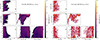 |
Fig. 5. Similar to Fig. 4 but for dBH-PMS. |
| In the text | |
|
Fig. 6. Example of a dBH-LC with a BH in the PISN range formed through triple evolution. In the upper panel, the yellow area and the red area represent the formation of the post-merger binary and the formation of the dBH-LC, respectively. In the lower panel, the gray area represents the phase when the inner binary undergoes MT. |
| In the text | |
|
Fig. 7. Two-dimensional birth rate distribution of MBH − Porb for dBH-MS formed through the IBM channel in triple evolution. This figure also shows one times, two times, and three times Gaia’s maximum observational baseline (10 years), which correspond to the cases where Gaia can at most fully resolve the entire orbit, half of the orbit, and one-third of the orbit, respectively. |
| In the text | |
Current usage metrics show cumulative count of Article Views (full-text article views including HTML views, PDF and ePub downloads, according to the available data) and Abstracts Views on Vision4Press platform.
Data correspond to usage on the plateform after 2015. The current usage metrics is available 48-96 hours after online publication and is updated daily on week days.
Initial download of the metrics may take a while.