| Issue |
A&A
Volume 706, February 2026
|
|
|---|---|---|
| Article Number | A232 | |
| Number of page(s) | 22 | |
| Section | Stellar structure and evolution | |
| DOI | https://doi.org/10.1051/0004-6361/202557456 | |
| Published online | 12 February 2026 | |
Self-lensing binaries as probes of supernova physics
1
Nicolaus Copernicus Astronomical Center, Polish Academy of Sciences Bartycka 18 00-716 Warsaw, Poland
2
School of Physics & Astronomy, University of Southampton Southampton Southampton SO17 1BJ, UK
3
Max Planck Institute for Astrophysics Karl-Schwarzschild-Straße 1 85748 Garching b. München, Germany
4
School of Mathematics, Statistics, and Physics, Newcastle University Newcastle upon Tyne NE1 7RU, UK
★ Corresponding author: This email address is being protected from spambots. You need JavaScript enabled to view it.
Received:
27
September
2025
Accepted:
3
December
2025
Abstract
Self-lensing (SL) in binary systems has the potential to provide a unique observational window into the Galactic population of compact objects. Using the startrack and COSMIC population synthesis codes, we investigate how different supernova mechanisms affect the observable population of SL systems, with particular attention to the mass gap (2–5 M⊙) in compact object distributions. We test three supernova remnant formation models with different convective growth timescales (fmix = 0.5, 1.0, and 4.0), simulating SL binary systems across the Galactic disk and bulge. We identify distinct groupings of SL sources based on lens mass and Einstein crossing time, clearly differentiating neutron star from black hole systems and close from wide orbits. Notably, the delayed fmix = 0.5 model predicts a significantly higher fraction of systems with lens masses in the mass gap region (up to about ten times more for certain surveys), suggesting that SL observations could help constrain this controversial population. Our analysis reveals a strong preference for systems with low centre-of-mass velocities (vcm ≤ 20 km/s) across all models, resulting primarily from physical processes governing compact object formation and binary survival. While many potential detections will have limited observational coverage, ZTF is predicted to yield several dozen well-covered systems that should enable detailed characterization. When applying simple detection criteria, including photometric precision and signal-to-noise requirements, predicted rates decrease by approximately two orders of magnitude but still yield up to a few tens of expected detections for LSST and ZTF in the Galactic disk population.
Key words: gravitational lensing: micro / methods: numerical / methods: statistical / binaries: general
© The Authors 2026
 Open Access article, published by EDP Sciences, under the terms of the Creative Commons Attribution License (https://creativecommons.org/licenses/by/4.0), which permits unrestricted use, distribution, and reproduction in any medium, provided the original work is properly cited.
This article is published in open access under the Subscribe to Open model. This email address is being protected from spambots. You need JavaScript enabled to view it. to support open access publication.
1. Introduction
The vast majority of the Galactic population of binary compact objects are expected to be part of relatively wide, non-interacting binary systems (Wiktorowicz et al. 2019; Olejak et al. 2020; Vigna-Gómez & Ramirez-Ruiz 2023). Some fraction of these are systems with non-compact companions, typically low-mass, main-sequence stars due to their long lifetimes. Self-lensing (SL) occurs when a compact lens in a binary system transits its normal (optically bright) companion star. The result is an amplification of the observed flux, the shape and amplitude of which depend on the mass of the lens, binary separation, impact parameter, projected size (radius) of the companion star, and limb darkening (Agol 2003). Self-lensing has been used to locate five white dwarf lenses to date, all within Kepler data (Kruse & Agol 2014; Kawahara et al. 2018; Masuda & Hotokezaka 2019), and it has been suggested that quiescent (non-accreting) neutron stars (NSs) and black holes (BHs) may also be detectable given the high cadence of new surveys, especially within the all-sky surveys of ZTF and the Vera C Rubin LSST (Wiktorowicz et al. 2021; see also Yamaguchi et al. 2024). Recent detailed simulations of TESS observations have demonstrated detection efficiencies of 4–7% for SL systems with compact companions from TESS Candidate Target List stars (Sajadian & Afshordi 2024). Similarly, Chawla et al. (2024) used the COSMIC binary population synthesis code to model SL detectability in detached BH binaries for TESS and Gaia, predicting only ∼1–4 and ∼76–102 detectable systems, respectively.
The potential of SL is only now being realized. Not only does the method avoid the biases inherent in other techniques – which tend to detect high-mass compact objects (thus precluding access to the low-mass gap) – but the numbers are potentially much larger than known X-ray binaries. This permits sensitive tests of supernova (SN) physics via correlations with kick velocity (Gandhi et al. 2019). In addition, as most lenses found this way are pristine, having never accreted matter from a companion star (Wiktorowicz et al. 2021), accessing their natal properties (mass and spin) can provide unique observational constraints on their formation mechanism. Binary interactions represent a critical uncertainty in the context of recent core-collapse SN theory (Burrows & Vartanyan 2021), as mass transfer can significantly alter SN progenitor structure (Burrows et al. 2024, 2025). Consequently, compact objects in SL binaries represent better observational constraints for investigating SN physics than, for example, X-ray binaries.
Recent years have seen the first predictions emerge for the population of SL systems in the Milky Way. These have relied on various iterations of binary population synthesis codes from Masuda & Hotokezaka (2019) and later Wiktorowicz et al. (2021, hereafter W21). The latter used the startrack population synthesis code (Belczynski et al. 2008), a realistic model for the Milky Way, and included NS lenses for the first time. In W21, the simulated population was folded through the key instrumental properties of the surveys, assuming a range of conditions, namely the initial mass function (IMF), star formation history, and the ‘Rapid’ SN model (Fryer et al. 2012; Belczynski et al. 2012). One of the main features of this SN model is that it reproduces the observational mass gap between NSs and BHs (around 2–5M⊙; Bailyn et al. 1998). However, observations – both from gravitational waves (Abbott et al. 2020) and spectroscopy (Jayasinghe et al. 2021) – have called into question the presence of such a gap. Should the gap truly contain systems, this may point to a ‘Delayed’ model for SNe, where the growth timescale of the Rayleigh-Taylor or convective instabilities that launches the explosion is relatively long (Belczynski et al. 2012).
W21 established the first comprehensive framework for predicting SL populations in optical surveys, demonstrating that ZTF, LSST, and TESS could detect hundreds to thousands of systems. Their analysis explored the impact of different IMF and detailed Galactic structure models on detection rates. However, W21 adopted a single SN remnant formation prescription, leaving open the question of how uncertainties in the explosion mechanism itself might affect the observable SL population. In this paper, we build on the results obtained by W21 to explore the impact of new developments in SN engine physics (Fryer et al. 2022) and the main characteristics of the SL population, including kick velocity distributions and – most importantly – whether objects in the mass gap can be recovered, pointing to a dominant SN mechanism. We follow the procedure outlined in W21 to calculate the expected population of SL objects in our synthetic populations of binaries. We choose to focus our analysis on those surveys with a high potential for detecting SL events due to their sky coverage, sensitivity, and cadence. Specifically, we include only the same survey instruments considered in W21: TESS, ZTF, and LSST (we refer the reader to W21 for a discussion of the various assumed instrumental characteristics such as duration, assumed cadence, and saturation.).
2. Methods
For this research, we utilized both the startrack and COSMIC population synthesis codes. We begin by introducing the startrack code, focusing on aspects particularly relevant for SL simulations. In Section 2.4, we describe the COSMIC code with emphasis on its differences compared to startrack.
2.1. Star formation history and initial conditions
We adopted the model of star formation rate (SFR) and metallicity distributions for the Galactic disk and bulge based on several observational constraints shown in Fig. 1–3 of Olejak et al. (2020) with two minor differences. First, we divided disk populations into ten instead of 11 sub-populations (with no separation for the Thin and Thick disk). Second, we assumed a solar metallicity of Z⊙ = 0.02 (instead of 0.014). We generated 15 stellar populations (ten for the disk and five for the bulge), which differ by their metallicity and age. The simulated numbers of systems were scaled to match the total stellar mass of the Milky Way disk and bulge (assumed to be 5.17 × 10¹⁰ M⊙ and 0.91 × 10¹⁰ M⊙, respectively; see Licquia & Newman 2015).
For the initial mass of the primary (the more massive star), we adopted a broken power-law IMF (Kroupa et al. 1993), following the standard formula: ξ(m) = (m/m0)−αi, where ξ(m)dm is the number of stars between masses m and m + dm. The exponent αi takes values of: α1 = −1.3 for M ∈ [0.08, 0.5] M⊙, α2 = −2.2 for M ∈ [0.5, 1.0] M⊙, and α3 = −2.3 for M ∈ [1.0, 150.0] M⊙.
The mass of the secondary (the less massive star) in the newborn binary is derived from the uniform mass ratio distribution in the range q ∈ [0.08/M1, 1]. For the initial orbital configuration, we adopted a period distribution following f(P)∝(log P)−0.55 and an eccentricity distribution f(e)∝e−0.42, consistent with the observational constraints from Sana et al. (2012) for massive binary systems. We normalized the stellar mass of the Galactic components, with the assumption of a high binary fraction for massive primary stars (with MZAMS > 10M⊙: 100%) and assumed that 50% of stars with M ≤ 10M⊙ are in binary systems (as motivated by observations, e.g. Moe & Di Stefano 2017).
2.2. Main assumptions on single and binary stellar astrophysics
Our Galactic population of binary systems hosting compact objects was generated using the startrack population synthesis code (Belczynski et al. 2008, 2020). The version of the code used in this study is the same as that described in Section 2 of Olejak et al. (2022). We adopted a strong pulsational-pair-instability/pair-instability SN, which limits the mass of BHs to ∼45 M⊙, as adopted in Belczynski et al. (2016). For non-compact accretors, we assumed a 50% non-conservative Roche lobe overflow with a fraction of the donor mass (1 − fa, where fa is the fraction of material transferred from the donor that is accreted onto the compact object) lost from the system, together with the corresponding part of the donor star and orbital angular momentum (see Section 3.4 of Belczynski et al. 2008). We also limited the mass accretion rate onto the non-compact accretor to the Eddington limit. For the stellar wind mass loss, we used formulae based on theoretical predictions of radiation-driven mass loss (Vink et al. 2001) with the inclusion of luminous blue variable mass loss (Belczynski et al. 2010). We adopted a Maxwell distribution of natal kicks, with σ = 265 km/s (Hobbs et al. 2005) lowered by fallback (Fryer et al. 2012) at NS and BH formation (see section 2.3). We adopted common envelope (CE) development criteria as described in section 5.2 of Belczynski et al. (2008), with the envelope ejection efficiency αCE = 1.0. We assumed that binary systems with Hertzsprung gap donor stars do not survive the CE phase (Belczynski et al. 2008), as stars with not well-developed convective envelopes are expected to merge (Klencki et al. 2021).
To calculate stellar remnant masses, we adopted the revised formulae given by Fryer et al. (2022) implemented as described in Section 2.2 of Olejak et al. (2022). In contrast to the previously used Rapid and Delayed SN models given by formulae 5 and 6 of Fryer et al. (2012), which may be treated as two extremes, the new formulae allowed us to test the impact of assumed convective growth timescales on the remnant masses (Mrem in units of M⊙). Equation 1 allowed us to calculate remnant masses assuming a smooth relation with a pre-SN carbon-oxygen core mass (MCO in units of M⊙; in startrack it is the value at the end of a star’s core helium burning phase), and by varying different mixing efficiencies (fmix, set by the convection growth timescale):
 (1)
(1)
where Mcrit = 5.75M⊙ is the assumed critical mass of the carbon-oxygen core for BH formation (the switch from NS to BH formation). In this work, we tested three variants of the formula with fmix = 0.5, 1.0, and 4.0, corresponding to models f05, f10, and f40. Models f05 and f40 correspond to the Delayed and Rapid models from Fryer et al. (2012), whereas f10 is an intermediate case. Note that the mass of the remnant was calculated using Equation 1 until some MCO value is reached, which depends on the steepness of the exponent (i.e. the adopted fmix value). If Mrem from Equation (1) exceeded the value of the total mass of the pre-SN star (Mpre − SN), then we assumed direct collapse of the star to a BH with mass-loss only in the form of neutrinos (1% of the pre-SN mass):
 (2)
(2)
We note that the fmix parameter, while capturing the dominant uncertainty related to convective growth timescales in the explosion mechanism (Fryer et al. 2022), represents a simplified treatment of the full complexity of core-collapse SN physics. Other physical uncertainties, including progenitor structure variations, explosion asymmetries, neutrino transport effects, and the inherently 3D and chaotic nature of the explosion (Burrows & Vartanyan 2021), may also influence remnant masses and natal kicks in ways not fully captured by this 1D parametrization. Binary evolution, especially the stellar winds, may also influence the final compact object masses and are not well constrained by available models.
In our simulations, NSs also formed via electron-capture SN (Hiramatsu et al. 2021) and are expected to possess relatively low masses and low natal kick velocities (Podsiadlowski et al. 2004) in contrast to core-collapse SN NSs, which are expected (and observed, e.g. Lyne & Lorimer 1994) to receive very large kicks as a result of an asymmetric neutrino-driven explosion. Following Belczynski et al. (2012, standard model) we assume that electron-capture SN NSs obtain no additional kicks due to asymmetric explosion (but the orbit may still be affected by the mass loss) and retain a post-SN mass of 1.26 M⊙.
We assume that the system does not change between SL flares. This should be true in general for the companion star, as the orbital period is far smaller than evolutionary timescales. However, precession resulting from flybys, which can be important also in sparse stellar systems such as the Galactic disk (Klencki et al. 2017), may destroy the fragile arrangement of system orbit and the observer.
2.3. Velocities
The centre-of-mass velocities of binary systems play a crucial role in determining their spatial distribution and detectability as SL sources. Systems that receive large natal kicks during SN explosions may be ejected from their birth locations, potentially reducing their detection probabilities in targeted survey regions.
We calculate the centre-of-mass velocity (vcm) for each binary using
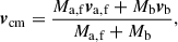 (3)
(3)
where Ma, f and va, f are the mass and velocity of the compact object (post-SN), and Mb and vb are the mass and velocity of the companion star.
We estimated each velocity component (vx, vy, vz) using (for derivation, see Section 6.3 of Belczynski et al. 2008)
 (4)
(4)
where vcm, bef is the velocity of the binary system before the SN explosion (equal to the rotational velocity around the Galaxy if this is the first SN) and
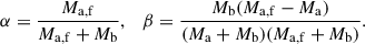 (5)
(5)
The first term in this equation relates to the asymmetric SN ejection, while the second term represents the Blaauw kick (Blaauw 1961) due to mass loss during compact object formation. Here, Ma is the pre-SN mass of the star, vprea, i is the relative velocity of the stars before the SN explosion, and vka, i is the natal kick velocity of the compact object after the SN (reduced by fallback). vcm, i represents only the additional velocity obtained through evolution, excluding Galactic rotation. We calculated the velocity magnitude as
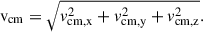 (6)
(6)
2.4. Cosmic
Given the substantial uncertainties and assumptions inherent in population synthesis modelling, we performed additional simulations using an independent code to assess the robustness of our results and quantify inter-code systematic uncertainties. We employed the Compact Object Synthesis and Monte Carlo Investigation Code (COSMIC), a binary population synthesis code adapted from the Binary Star Evolution code (BSE; Hurley et al. 2002) with updated evolution prescriptions and parameters (Breivik et al. 2020). The evolutionary prescriptions are broadly consistent with those implemented in startrack, though some key differences exist as outlined below.
For the primary star initial mass distribution, we adopted the same broken power-law IMF described in Section 2.1, with an additional regime for the lowest masses: α0 = −0.3 for M ∈ [0.01, 0.08]M⊙. The secondary star mass was sampled from a uniform mass ratio distribution q ∈ [M2, min/M1, 1], where (and unlike with startrack) M2, min is constrained such that the pre-main-sequence lifetime of the secondary does not exceed the total lifetime of the primary (assuming single-star evolution). Orbital periods and eccentricities, similarly to startrack, follow the observational distributions from Sana et al. (2012).
Stellar winds were computed using theoretical prescriptions for radiation-driven mass loss and luminous blue variable episodes (Vink et al. 2001; Vink & de Koter 2005). Wind velocities and mass accretion rates are consistent with startrack implementations, with accretion rates onto the NS or BH limited to the Eddington rate.
Mass transfer stability follows the prescriptions of Hurley et al. (2002), with critical mass ratios consistent with standard BSE formulations. Distinct stability criteria were applied for giant stars following Hjellming & Webbink (1987).
Common envelope evolution employs the standard αλ formalism with an ejection efficiency parameter αCE = 1.0. The binding energy factor λ is calculated using the method of Pols et al. (1995). Following the startrack simulations, we adopted a ’pessimistic’ CE scenario where mergers are inevitable when unstable mass transfer occurs in systems with ill-defined core-envelope boundaries (Klencki et al. 2021).
We implemented two SN mechanisms representing the extremes of convective mixing efficiency: the ‘Delayed’ and ‘Rapid’ explosion models of Fryer et al. (2012) (equivalent to models f05 and f40, respectively). For remnant mass determination, we applied a maximum mass loss of 0.5 M⊙ due to baryonic-to-gravitational mass conversion. This limit applies when the compact object progenitor core mass ≥11 M⊙, corresponding to complete fallback scenarios where natal kicks, are governed by neutrino emission and are therefore negligible.
Natal kicks are drawn from Maxwellian distributions with velocity dispersions of
-
σ = 265 km s−1 for Fe core-collapse SN;
-
σ = 20 km s−1 for electron-capture and ultra-stripped SN (progenitor mass range 1.6–2.25 M⊙).
The above prescriptions follow Hobbs et al. (2005). While recent observations suggest some BHs may receive significant natal kicks comparable to NSs (e.g. Atri et al. 2019; Fragione et al. 2022), we maintained consistency with startrack by moderating kicks through fallback effects, resulting in negligible kicks for massive compact object progenitors.
2.5. Self-lensing description
The SL calculations in this work follow the methodology established in W21. Simulated binaries were randomly positioned in the Galactic potential, as described in Wiktorowicz et al. (2020), with positions used to calculate apparent magnitudes for each system as observed from Earth (positioned 8.3 kpc from the Galactic centre and 20 pc above the Galactic plane). Binary inclinations were sampled uniformly in cos i, ensuring isotropic orbital orientation distributions. Uncertainty estimates were established using bootstrap resampling with 12 iterations with results reported as means and standard errors (1-σ). For each bootstrapping sample, the systems received different Galactic positions and inclinations.
For each system, the lensing amplitude μsl was calculated using the analytic framework of Witt & Mao (1994), which accounts for the finite size of the source star and the impact parameter (see W21 for details). The effective crossing time τeff was defined as the duration during which at least a fraction of the companion star’s disk falls within the Einstein radius of the compact object, incorporating realistic impact parameters rather than assuming edge-on geometries (see equation (5) of W21).
A crucial distinction in this work concerns the definition of ‘detectable’ SL events. By ‘detectable’ we mean systems for which at least one photometric observation can be made during the SL event, where an SL event is defined as the time period when any part of the companion star’s disk falls within the Einstein radius of the compact object, given a particular survey’s observing strategy. The basic observational requirements we imposed include: (1) geometric alignment such that the compact object transits the companion star from Earth’s perspective; (2) at least one survey observation temporally coinciding with the lensing event given the survey’s cadence; and (3) the source star being detectable above the survey’s limiting magnitude (msource < mlim, where mlim = 21, 24, and 12 for ZTF, LSST, and TESS, respectively, as detailed in W21 Table 1).
In fact, this criterion does not require distinguishing the event from other astrophysical phenomena such as stellar flares, ellipsoidal variations, and outbursts, nor does it account for the detectability of the lensing signal above the photometric noise level of the host star. We did not require sufficient observations to characterize the lensing light curve shape, nor definitive identification of the event as SL rather than other forms of variability. This permissive definition was chosen to establish an upper limit on observable systems that is largely independent of detailed assumptions about photometric noise characteristics, event identification algorithms, and false-positive rates. Experience from Kepler, where detailed searches examined thousands of candidate variable stars to identify just four confirmed white dwarf SL systems (Kruse & Agol 2014; Kawahara et al. 2018; Masuda & Hotokezaka 2019), suggests that the vast majority of photometric transients will be other astrophysical phenomena or instrumental artefacts.
The analysis presented in Section 3 considers all systems meeting this basic observational requirement, providing upper limits on detectable populations. More conservative and realistic predictions accounting for photometric noise thresholds, signal-to-noise requirements, and filter-specific detectability are discussed in Section 4, where we apply criteria closer to what would enable actual SL identification.
3. Results
3.1. Intrinsic distribution of masses
Figs. 1 and 2 show the intrinsic mass distributions of compact objects (the lenses) and their non-compact companions in Galactic binary systems. We present results for three SN models with fmix = 0.5, 1.0, and 4.0 using startrack, while Fig. 3 and 4 show the Delayed and Rapid models for COSMIC.
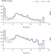 |
Fig. 1. Intrinsic mass distribution of Galactic NSs and BHs in binaries with non-compact companions from startrack. Top panel: Bulge sources. Bottom panel: Disk sources. |
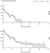 |
Fig. 2. Intrinsic mass distribution of non-compact binary companions in Galactic systems from startrack. Top panel: Bulge sources. Bottom panel: Disk sources. |
The higher metallicity in the bulge compared to the disk (Section 2.1; Olejak et al. 2020) produces a noticeable decrease in the ratio of BHs to NSs; otherwise, both distributions are similar. The rapid convective growth model (fmix = 4.0 or Rapid) creates a prominent mass gap between 2–7M⊙. In contrast, the fmix = 0.5 model efficiently produces massive NSs and low-mass BHs within this range. The intermediate model (fmix = 1.0) produces a gap that is less pronounced than the fmix = 4.0 case. Overall, startrack and COSMIC distributions are comparable.
The non-compact companion mass distributions are largely independent of the SN model choice, differing only in absolute numbers. The fraction of massive non-compact companions is lower in the bulge due to enhanced stellar wind mass loss at higher metallicity.
Figure 5 and 6 focus on the NS mass distributions. The prominent peak at 1.26 M⊙ corresponds to NSs formed via electron-capture SN, enhanced by our assumption of zero natal kicks for such events. The fmix = 0.5 (Delayed) model differs significantly from other models in producing more massive NSs (≳1.5 M⊙) and mass gap objects (≳2 M⊙).
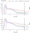 |
Fig. 5. Intrinsic mass distribution of Galactic NSs (Mlens < 2.5 M⊙) in binaries with non-compact companions. This shows a focused view of the NS population from Figure 1. |
3.2. Self-lensing
Table 1 presents our predictions for detectable SL events across different surveys and Galactic components. We used bootstrap resampling with 12 iterations to establish uncertainty estimates, reporting means and standard errors (1-σ) for each model configuration. These results do not account for filter effects or the detectability of flares above the noise level (see Section 4).
Predicted number of detectable SL events.
Several clear trends emerge from our analysis. ZTF consistently shows the highest detection potential across all models, with predicted yields of ∼6300 detectable SL events for the disk using the f05 model. The following rankings directly reflect the survey characteristics detailed in W21 Table 1: ZTF’s combination of 5-year baseline and daily cadence maximizes the number of opportunities to capture short-duration SL events; LSST’s 10-year duration with 4.6-day cadence provides excellent long-term coverage but samples events less frequently; while TESS’s limited effective exposure time per field (∼2 months) significantly restricts its sensitivity to systems with longer orbital periods. LSST is the second most productive survey with ∼3200 disk events, while TESS shows the lowest yields at ∼590 events. This ranking holds regardless of the binary population model or Galactic component considered, and is consistent with previous findings from W21.
The Galactic disk consistently produces significantly more detectable events than the bulge – approximately an order of magnitude more across all surveys and models. For example, ZTF predictions range from ∼370 bulge events to ∼6300 disk events for the f05 model, while LSST shows ∼150 bulge events compared to ∼3200 disk events.
Among our SN models, the f05 model predicts the highest numbers of detectable SL events for disk populations, while the three models yield comparable results for bulge populations. The Delayed COSMIC model generally produces results comparable to our f40 model, though with somewhat more events than f05. This difference is most pronounced for the disk component in LSST and TESS observations, where COSMIC predicts approximately 50% more events in Delayed than startrack in f05.
The Delayed SN mechanism (f05) consistently produces more observable SL binaries than the Rapid mechanism (f40), particularly in disk populations across both startrack and COSMIC simulations and primarily in the low Mlens (≲10 M⊙) regime (see Table 1). This differential response suggests the relative distribution between disk and bulge components could provide valuable constraints on SN mechanisms.
While our analysis identifies potentially detectable events, limited temporal coverage or insufficient orbital repetitions during a survey’s operational period may prevent definitive classification (see Section 3.4). However, these candidates remain valuable targets for follow-up radial velocity measurements to independently confirm their nature (McMaster et al., in prep.).
Fig. A.1 compares key system parameters from startrack results across the tested SN models and observing instruments, with separate lines for the Galactic disk and bulge. The Mlens distributions exhibit notable differences between fmix values, reflecting variations in the underlying intrinsic distributions (see Fig. 1). The peak at ∼35 M⊙ in the ZTF’s Mlens distribution likely results from a single high-probability system that obtained significant observational weight by chance.
TESS shows enhanced sensitivity to massive companions (≳10 M⊙), for which the effective Einstein crossing time (τeff) is characteristically short (≲10−2 yr). These close binaries have very short periods that can be effectively sampled only by TESS with its high cadence. Notably, all parameter distributions except Mlens show minimal dependence on the adopted SN model. Similar conclusions can be drawn from the COSMIC results (Fig. A.2).
3.3. Mass Gap objects
Table 2 presents predictions for SL systems in the mass gap (2–5M⊙). ZTF exhibits the highest detection rates and provides the strongest discrimination between SN engine models, with startrack f05 yielding about ten times more detections than f10 in the disk component. LSST yields substantially fewer mass gap detections compared to ZTF primarily due to its lower observing cadence (4.6 days versus 1 day; see W21 Table 1), which reduces the probability of obtaining observations during short-duration lensing events. We note that photometric precision is not a factor in these ‘raw’ detection numbers, as noise thresholds are only applied in Section 4. TESS shows the most limited potential for mass gap discoveries, particularly in the bulge, where rates drop to < 1 expected detections for several models.
Results for the mass gap systems.
The COSMIC results generally predict lower numbers of expected detections than startrack, with differences up to a factor of 5. This disparity reflects the different prescriptions for SN engines, making this lens mass range of Mlens ≲ 10 M⊙ particularly sensitive to the choice of evolutionary codes. The primary differences between the codes in this mass range stem from distinct implementations of the SN remnant mass formulae:startrack uses the Fryer et al. (2022) prescriptions, while COSMIC uses the earlier Fryer et al. (2012) formulations. While the intrinsic mass distributions from the two codes are qualitatively similar (Figs. 1, 3), modest quantitative differences, particularly in the 2–5 M⊙ mass gap region, can become amplified when convolved with observational selection effects. Although startrack’s f05 and f40 models are counterparts of COSMIC’s Delayed and Rapid models, respectively, the prescriptions differ, which may account for the observed differences in estimated numbers of detections. Furthermore, this range of mass is particularly susceptible to evolutionary effects such as SN explosions and natal kicks, which may be sources of additional differences between the models.
Fig. A.3 presents the same parameter distributions as Fig. A.1, but focuses exclusively on systems with lens masses (Mlens) between 0 and 10 M⊙. The distributions exhibit similar overall trends to those observed in the complete population. However, notable differences between models emerge primarily in the Mlens distributions (this distinction is also evident in the COSMIC data shown in Fig. A.4). Compared to the entire population, the subset of lenses with low τeff values is more pronounced in this mass range. Beyond this effect, the primary observable difference remains the enhanced detection frequency characteristic of the f05 model.
3.4. Coverage and recurrence
Self-lensing events in binary systems present unique observational challenges and opportunities. The detectability and characterization of these events depend critically on the observational coverage of individual events and their recurrence over time. In this section, we analyse the implications of our model predictions for various survey instruments, focusing on two key aspects: the number of observations per SL event and the frequency of recurring events for each system. We also introduce a combined metric to assess the overall observability of SL systems across different surveys. This analysis provides crucial insights into the practical limitations and potential strategies for detecting and studying SL events in large-scale astronomical surveys.
Table B.1 presents the results of our simulations for different surveys, obtained by imposing observational cuts (limiting magnitudes, cadence, etc.) on the simulated data (see W21 for details). We introduce two important parameters: coverage (ncov) and recurrence (nrec).
Coverage (ncov) represents the minimum number of observational data points covering a single SL event. Higher coverage increases the likelihood of identifying the event with SL and estimating a corresponding magnification and Einstein crossing time. Our results show that the predicted number of sources drops rapidly with increasing ncov (Table B.1), indicating that most SL events will have limited coverage and may be difficult to distinguish from other types of outbursts.
Recurrence (nrec) represents the number of recurring SL events for a single source expected during the survey. Recurrence is a key differentiating factor between SL and micro-lensing events, the latter being one-time occurrences. The main factor limiting nrec is survey duration. Long-term surveys such as LSST and ZTF are more likely to observe multiple events from a single system, whereas short-duration surveys such as TESS (effective duration < 2 months) will observe only a few systems with multiple events. In reality, nrec may be affected by factors that change orbital alignment or system position, such as flybys or precession.
Imposing higher minimum thresholds for coverage and recurrence progressively reduces the number of systems meeting the detection criteria. However, higher values for both can improve identification through increased observations during peak magnification. We introduce a parameter, ntot, describing the total number of observations of lensing events per source during the entire survey duration:
 (7)
(7)
Table B.2 summarizes our results for different thresholds of ntot. LSST is capable of detecting a few tens of well-covered (ntot > 50) SL systems, which should allow for better inference of curve features and tighter constraints on system parameters (e.g. Kruse & Agol 2014). For LSST and ZTF, we observe a statistically significant difference between predictions for different SN models, where the differences exceed the 1σ bootstrap uncertainties, which becomes more pronounced with higher ntot thresholds.
3.5. Clustering of self-lensing systems
Fig. 7 illustrates the relationship between τeff and Mlens for ZTF’s Galactic disk predictions with the f40 model. Three distinct groups of objects are evident:
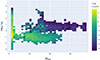 |
Fig. 7. Relationship between effective Einstein crossing time (τeff) and lens mass (Mlens) for the Galactic disk population in ZTF observations with f = 4.0. Other models, instruments, and Galactic components are presented in Fig. A.5. |
-
𝒢BH, short: Higher-mass, short-duration systems (Mlens > 2 and τeff < 1 day);
-
𝒢BH, long: Higher-mass, long-duration systems (Mlens > 2 and τeff ≥ 1 day);
-
𝒢NS: Lower-mass systems (Mlens ≤ 2).
All SN models exhibit similar patterns (Fig. A.5), with the mass gap region (Mlens ∈ [2, 5]) most prominently populated in the f05 model and least populated in the f40 model. While TESS results follow comparable trends, the lower predicted number of SL sources makes these patterns less distinct.
Table 3 summarizes the weighted properties (mostly 10%, 50%, and 90% percentiles) of each population (all simulations together), revealing the following distinctive characteristics beyond just Mlens and τeff:
-
The 𝒢NS population features more massive source stars compared to the 𝒢BH, short and 𝒢BH, long groups.
-
𝒢NS systems exhibit the highest magnifications (⟨μsl, max⟩), though the majority (∼80%) show modest magnifications (μsl ≲ 2).
-
Although 𝒢NS can have much higher centre-of-mass velocities (up to ∼500 km/s), both 𝒢BH, short and 𝒢BH, long populations have higher median values (⟨vcm⟩), suggesting greater resilience to natal kicks due to their more massive compact objects.
-
All populations display similar typical number of data points per SL event (coverage; ncov) and typical number of recurring SL events per source during survey duration (recurrence; nrec). See Section 3.4.
-
The 𝒢BH, long population, characterized by longer τeff, the consequence of longer orbital periods (Porb), shows substantially higher magnification (μsl) than the 𝒢BH, short population.
While most systems have relatively low recurrence rates, the few systems with higher nrec (see Section 3.4) significantly influence the weighted median due to their enhanced detectability. The elevated typical total coverage count (ntot) directly results from the high typical recurrence values.
Properties of SL sources.
The systems with the highest magnifications typically harbour low mass main-sequence source stars (Msource ≲ 0.5 M⊙) on very wide orbits (Porb > 10 kyr). Such systems will have a very low observation probability, and their configurations will probably be unstable due to dynamical interactions (Klencki et al. 2017).
3.6. Velocity in detail
Fig. 8 presents the centre-of-mass velocity (vcm) distributions of SL sources for different SN engines and surveys, separated by Galactic component. The distributions show minimal variation between SN engines for the same survey. Notably, despite the lower predicted number of systems in the bulge compared to the disk, their velocity distributions remain similar. Any differences observed in the high-velocity tails (vcm > 300 km/s) are statistically insignificant due to limited sample sizes. The distributions are dominated by low-velocity systems (≲20 km/s), primarily representing BHs with significant or complete fallback, and NSs receiving low kicks from the assumed, underlying Maxwell distribution.
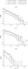 |
Fig. 8. Centre-of-mass velocity (vcm) distributions for SL binaries for different SN engines and surveys, separated by Galactic component (disk and bulge). |
Fig. 9 illustrates the differences in velocity distributions between surveys. While LSST and ZTF show similar distributions (with ZTF predicting higher absolute numbers of sources), TESS exhibits a distinct cut-off around 300 km/s with few systems beyond this threshold. This cut-off occurs because rapidly moving systems typically form wide, eccentric binaries that are rarely captured by TESS’s limited exposure time per sky region. As expected, these survey-dependent characteristics remain consistent across all SN models and Galactic components.
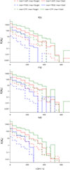 |
Fig. 9. Centre-of-mass velocity (vcm) distributions comparing different surveys (LSST, ZTF, and TESS) for each SN engine and Galactic component. |
The predominance of low-velocity systems (≲20 km/s) stems from a fundamental selection effect: binaries experiencing smaller natal kicks are more likely to remain gravitationally bound. Consequently, more massive SN remnants – which undergo significant fallback or direct collapse with minimal momentum kicks – are preferentially preserved as binary systems. Similarly, NSs formed through electron-capture SN, which receive no natal kicks in our simulations, have higher survival rates in binaries compared to NSs formed through core-collapse SN, which typically receive kicks exceeding 100 km/s (see Section 2.2). Therefore, the velocity distribution reflects the physical expectation that most detectable SL events will occur in binaries that have experienced minimal disruption from SN kicks.
Fig. A.6 illustrates the relationship between lens mass (Mlens) and centre-of-mass velocity (vcm) across all models. Our findings are consistent with the anti-correlation between BH mass and peculiar velocity reported by Gandhi et al. (2019). While they identified this trend in Galactic BH X-ray binaries using Gaia DR2 data (finding a slope of  km s−1 M⊙−1 with 99.9% confidence in the anti-correlation), our models extend this relationship across a broader mass spectrum showing similar trend. We similarly observe that systems with massive lenses (≳40 M⊙) exhibit minimal velocities (≲1 km/s), while the highest velocities (≳100 km/s) correspond to lower-mass lenses (≲10 M⊙), predominantly NSs. Notably, Gandhi et al. (2019) observe peculiar velocities of 50–150 km/s for several systems in this mass range, further strengthening the inverse relationship between compact object mass and system velocity. Interestingly, SL binaries containing mass gap lenses (∼2–5 M⊙) display higher average velocities compared to other SL systems, which results from higher natal kicks from core-collapse SNe and lower fallback.
4. Conservative detection limits
The values presented throughout this paper are considered raw detection estimates because they do not account for the specific limitations of filter bandwidth or flare detectability caused by noise. In this section, we address this by applying additional constraints.
4.1. Apparent magnitude calculations
To determine the apparent magnitudes of stars in SL binary systems, we employed a synthetic photometry approach using blackbody radiation profiles and instrument-specific filter responses. Filter transmission curves were obtained from the Filter Profile Service1 for the relevant instruments.
For each source star, we assumed blackbody radiation characterized by the stellar effective temperature Teff. The spectral energy distribution was calculated using the Planck function
 (8)
(8)
where h is Planck’s constant, c is the speed of light, k is Boltzmann’s constant, and λ is the wavelength.
The observed flux density at Earth was computed by scaling the blackbody flux by the geometric dilution factor
 (9)
(9)
where R★ is the stellar radius and D is the distance to the system.
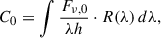
The photon count rate through each filter was calculated by integrating the product of the flux density and filter response function R(λ) over wavelength:
 (10)
(10)
The apparent magnitude was then computed as
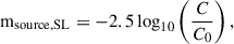 (11)
(11)
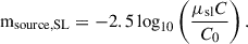
where C0 is the zero counts reference point calculated as
 (12)
(12)
where Fν, 0 = 3631 × 10−26 [W m−2 Hz−1].
For SL events, the magnified apparent magnitude was computed by multiplying the flux by the magnification factor μsl before conversion to magnitude:
 (13)
(13)
We did not include interstellar extinction in our apparent magnitude calculations, following the approach of W21. This simplification was motivated by the expectation that the majority of detectable SL systems are relatively nearby where optical extinction is modest. In fact, incorporating detailed 3D extinction maps (e.g. Green et al. 2019) would add significant computational complexity without substantially affecting our primary goal of comparing relative detection rates between SN models, as extinction is expected to affect all models similarly.
4.2. Flare detection criteria
In the simplest case (i.e. in the absence of stellar noise–see Ward et al., in prep, for more detailed simulations), the detectability of SL flares depends on both system visibility and the photometric precision of the observing instrument. We applied two fundamental criteria for flare detection:
-
System Visibility:
The source star must be detectable above the instrument’s limiting magnitude
 (14)
(14)where mlim is the limiting magnitude for each survey in each single observation. This condition was already included in W21 predictions (see their table 1) and in the raw results throughout the paper. We note that this is a rather conservative limitation and can be improved, for example, by stacking observations.
-
Flare Detectability:
The magnification during the SL event given by
 (15)
(15)must produce a photometric signal exceeding X σ above the quiescent stellar flux. In the above, msource, SL is the apparent magnitude during the SL event (calculated using the magnification factor μsl as described in Section 4.1), and σnoise is the survey-specific photometric uncertainty at that magnitude.
The photometric noise levels vary significantly between instruments; for LSST, we adopted a uniform photometric precision of σnoise = 10 mmag based on the survey specifications2; for ZTF, we assumed a conservative estimate of σnoise = 25 mmag (Masci et al. 2019); for TESS, the photometric uncertainty depends on the source brightness (Sullivan et al. 2015; Oelkers & Stassun 2018). We utilized the empirical noise model (σnoise(T)) from Oelkers & Stassun (2018)3, which provides noise estimates in parts-per-million (ppm) as a function of apparent magnitude. The conversion from parts per million to millimagnitudes and from 1-hour to 1-minute exposures is
![Mathematical equation: $$ \begin{aligned} \begin{split} \sigma _{\text{noise,TESS}}(T) \text{[mmag]}&= \frac{\sigma _{\text{ noise}}(T) \text{[ppm]}}{1000} \times \sqrt{\frac{1\,\text{ h}}{1\,\text{ min}}} \\&\approx 0.0077 \times \sigma _{\text{ noise}}(T) \text{[ppm]}, \end{split} \end{aligned} $$](/articles/aa/full_html/2026/02/aa57456-25/aa57456-25-eq41.gif) (16)
(16)
where T is TESS magnitude.
Additionally, we applied a noise correction for all instruments to account for multiple detections as
 (17)
(17)
where ntot is the total number of flare data points during the entire survey (including multiple detections of the same flare and repeating events; see Section 3.4).
4.3. Conservative predictions
Table 4 compares predicted stellar lensing event rates under different observational constraints: filter-only selections, where the flux is calculated within the instrumental band and SL is detected at > 0 σ (nsl, filter only), versus more conservative S/N thresholds (nsl, 2σ and nsl, 3σ). As expected, the results demonstrate substantial reductions in detectable events with respect to mere detections (Table 1). For LSST, the transition from filter-only to 3σ limited detections reduces event rates by approximately 30–40% across all models and Galactic components. TESS exhibits the most severe reduction, with 3σ limited predictions showing order-of-magnitude decreases compared to filter-only predictions, particularly for bulge observations. ZTF shows intermediate behaviour, with 3σ limited predictions typically reduced by 50–60% relative to filter-only predictions.
Detection rates of SL events.
Comparing the two population synthesis codes, COSMIC generally predicts higher event rates than startrack, particularly for disk observations. For LSST disk observations, COSMIC predictions exceed startrack by factors of 3 to 4. However, both codes show similar trends in the relative impact of S/N constraints, with the most stringent 3σ threshold reducing detection rates substantially across all instruments as expected.
The impact of S/N constraints is particularly pronounced for mass gap systems, where 3σ limited predictions show dramatic reductions compared to unconstrained scenarios. For the f05 or Delayed model, all three surveys converge to similar expectations of approximately 0.1 ± 0.1 detections. For the f40 or Rapid model, the rates are 3.5 × 10⁻³, 7.1 × 10⁻³, and 2.8 × 10⁻⁵ expected detections for LSST, ZTF, and TESS, respectively, highlighting the extreme difficulty of observing mass gap stellar lensing events with current survey capabilities and stringent detection thresholds.
Table B.3 presents a comprehensive comparison of median system properties between events detectable above the 3σ threshold (Yes) and those falling below this detection limit (No). The analysis reveals distinct systematic differences in the physical and observational characteristics of detectable versus undetectable systems.
Detectable systems consistently exhibit shorter effective Einstein crossing times across all instruments and Galactic components. For LSST and ZTF, detectable systems show ⟨τeff⟩∼0.05 − 0.06 [day] compared to ⟨τeff⟩∼0.18 − 0.43 [day] for undetectable systems. TESS shows a less pronounced but similar trend, with detectable systems having ⟨τeff⟩∼0.04 − 0.18 versus ⟨τeff⟩∼0.26 − 0.35 for undetectable events. Two effects are responsible for this trend. Systems with lighter compact object progenitors frequently become unbound due to natal kicks. Additionally, shorter orbital periods facilitate detections due to more frequent SL flares within survey durations, which counteracts the effect of shorter flare durations.
A striking contrast emerges in lens masses: detectable systems are associated with significantly more massive BH lenses (⟨Mlens⟩∼14 − 16 M⊙) compared to undetectable systems (NS with ⟨Mlens⟩∼1.2 − 1.5 M⊙). Conversely, detectable systems tend to have lower source masses, with ⟨Msource⟩∼0.6 − 0.7 M⊙ versus ⟨Msource⟩∼1.7 − 4.1 M⊙ for undetectable systems, although both are typically main-sequence stars.
Detectable systems exhibit significantly longer orbital periods, particularly evident in ZTF observations where ⟨Porb⟩∼26 − 39 days for detectable systems compared to ⟨Porb⟩∼2.4 − 4.1 days for undetectable systems. LSST shows a similar but less extreme trend. The distance distributions show that detectable systems are generally located at smaller distances (⟨d⟩∼7 − 9 kpc) compared to undetectable systems (⟨d⟩∼9.2 − 9.8 kpc).
Detectable systems are associated with dimmer apparent source magnitudes (⟨msource⟩∼20 − 22 mag) compared to undetectable systems (⟨msource⟩∼12 − 17 mag). The situation is opposite for TESS where the detectable systems are typically brighter than the undetectable ones. This counter-intuitive trend for LSST and ZTF arises because low-mass companions are much more abundant than high-mass ones and, being physically smaller, produce higher peak magnifications during lensing events (see W21; Fig. 1). These stronger magnification events can be detected even when the baseline source is dim. In contrast, TESS’s photometric precision degrades significantly for fainter sources, making it preferentially sensitive to brighter systems (see Section 4.2).
The total number of observational points shows instrument-specific patterns. For LSST and ZTF, detectable systems receive fewer total observations (⟨ntot⟩∼2 − 5) compared to undetectable systems (⟨ntot⟩∼22–24 or 90–110 for LSST and ZTF, respectively). TESS exhibits the opposite trend with much higher observation totals for both categories.
These results highlight the complex interplay between system properties and detection thresholds in lensing surveys. The preference for massive lenses, shorter crossing times, and specific orbital configurations in detectable systems provides important constraints for optimizing survey strategies and interpreting observational results. The instrument-specific detection biases revealed in this analysis – particularly the systematic differences in observable system properties between detectable and undetectable events – must be carefully considered when comparing theoretical predictions with observational constraints from different survey programs.
However, several factors could potentially increase these conservative detection rates significantly. Extended survey durations beyond the baseline observing programs would accumulate more photometric data points and improve S/N for marginal events. Similarly, combining observations from multiple surveys could enhance detection rates and confidence. More sophisticated Milky Way models, as demonstrated in W21, can predict higher event rates (up to five times) through more accurate treatments of stellar populations (e.g. metallicity distribution, IMF) and compact object distributions (Milky Way model, density profiles instead of snapshots, etc.). Advances in noise reduction techniques and data processing algorithms could lower effective detection thresholds, while relaxing magnitude limits to include fainter sources would expand the observable target population. Furthermore, promising stellar lensing candidates identified through photometric surveys could be confirmed through follow-up radial velocity observations, converting marginal photometric detections into secure confirmations. These considerations suggest that our predictions represent conservative lower bounds.
5. Discussion
5.1. Comparison with Wiktorowicz et al. (2021)
Our study extends the work of W21 by specifically investigating how different SN engines influence the population of compact objects in binary systems detectable through SL. While we employed a simplified Galactic model consisting of only the thin disk and bulge components, this simplification is justified, as W21 demonstrated that other Galactic components contribute minimally to the overall mass and do not significantly affect SL detection rates. Similarly, our adoption of the star-formation history and chemical evolution model from Olejak et al. (2020) streamlines calculations without compromising the validity of our conclusions.
Both studies reach similar conclusions regarding the relative detection capabilities of different surveys. ZTF and LSST consistently emerge as more promising platforms for SL detections compared to TESS (cf. Table 2 in W21), primarily due to their extended survey durations and superior sensitivities.
The detection rates predicted by our study, particularly for the disk population under the f05 model, fall approximately within the lower range of the broader predictions presented in W21 for various IMFs (LSST: 5000–14 000; ZTF: 2000–5500; TESS: 60–170; see W21 Table 1). This quantitative difference likely stems from our simplified Galactic model and specific evolutionary assumptions, compared to the more detailed Milky Way model employed in W21.
Our analysis reveals a strong preference for SL systems with low centre-of-mass velocities (vcm), consistent with the physical understanding that binaries experiencing significant natal kicks have a lower probability of remaining bound and subsequently detectable. While W21 implicitly incorporated natal kick effects on binary survival, our study explicitly examines vcm distributions across different SN models, providing new insights into this relationship.
In summary, while our results align with W21 regarding overall survey detection trends, our study contributes novel insights into aspects not previously explored in depth. Specifically, we illuminate the critical influence of different SN formation mechanisms on SL detectability and characterize the properties of SL systems within the mass gap. These findings, enabled by our focused methodology, complement the broader scope of W21 and advance our understanding of SL binary populations.
5.2. Comparison between startrack and COSMIC results
Our analysis employs two independent binary population synthesis codes to assess the robustness of our SL predictions and quantify inter-code systematic uncertainties. The specific implementations of the same physical processes may differ and be subject to different optimization. While both codes share similar evolutionary prescriptions, several key differences in their implementations provide valuable insights into model dependencies and systematic uncertainties in our results.
The primary differences between startrack and COSMIC lie in their treatment of specific evolutionary phases and physical prescriptions. COSMIC adopts a slightly extended IMF, incorporating an additional low-mass regime (α0 = −0.3 for M ∈ [0.01, 0.08] M⊙) compared to the standard broken power-law used in startrack. The secondary mass sampling also differs, with COSMIC employing a uniform mass ratio distribution constrained by pre-main-sequence lifetime considerations, while startrack uses its own prescription for binary mass ratios.
The SN mechanisms represent the most significant difference in our comparison. startrack employs three convective mixing models (f05, f10, f40 corresponding to fmix = 0.5, 1.0, 4.0; Fryer et al. 2022), while COSMIC uses the ‘Delayed’ and ‘Rapid’ explosion models (Fryer et al. 2012) that roughly correspond to the f05 and f40 extremes, respectively. The Rapid convective growth models (f40 or Rapid) consistently create a prominent mass gap between 2–5 M⊙ in both codes, while the delayed models (f05 or Delayed) efficiently populate this region with massive NSs and low-mass BHs. Minor differences in the detailed shape of the mass distributions of lenses and sources likely reflect the subtle differences in evolutionary prescriptions and numerical implementations between the codes. However, these variations are well within the expected range of systematic uncertainties inherent in population synthesis modelling.
Table 1 reveals that COSMIC generally predicts fewer detectable SL events than startrack, particularly for disk populations. The most significant discrepancy occurs in the ZTF disk predictions, where COSMIC yields approximately 60% fewer events than the startrack f05 model (2700 vs 6300 events). However, COSMIC results align more closely with the startrack f40 model, suggesting that the delayed versus rapid SN mechanisms represent the primary source of inter-code variation. For bulge populations, the agreement between codes is much better.
The ranking of surveys by detection potential remains consistent across both codes: ZTF shows the highest numbers, followed by LSST, then TESS. This reflects the same prescriptions used in post-processing for analysis of both code results.
The consistent qualitative trends across both codes – including the survey ranking, disk/bulge ratios, and parameter distribution shapes – provide confidence in our main conclusions. However, the quantitative differences warrant careful consideration regarding the use of absolute detection rates for distinguishing between SN models.
The inter-code systematic uncertainties in predicted absolute detection rates are substantial, typically factors of ∼1.5–2. Importantly, these systematic differences are comparable to, or in some cases exceed, the differences between adjacent SN models (e.g. f10 vs f40). This overlap suggests that distinguishing between similar SN mechanisms based solely on absolute event counts may be challenging given current systematic uncertainties inherent in binary population synthesis.
Population synthesis codes represent our current understanding of stellar and binary evolution, but they are developed independently with different numerical implementations and physical prescriptions at varying levels of sophistication. While we cannot exhaustively analyse all sources of uncertainty in population synthesis modelling, comparing independent codes provides valuable insights into the magnitude of these systematic effects.
6. Conclusions
Using the startrack and COSMIC population synthesis codes, we investigated how different SN engines affect the observable population of SL binary systems in the Milky Way. Our analysis reveals several key findings that advance our understanding of compact object populations and their detectability through SL.
Our models predict substantial numbers of detectable SL events across major astronomical surveys. For the Galactic bulge, we expect 21 to 650 events, while the Galactic disk should yield 370 to 6300 events depending on the survey and SN model. ZTF consistently shows the highest detection potential, followed by LSST, then TESS. This ranking remains robust across all SN models and reflects fundamental differences in assumed survey duration, cadence, and sky coverage.
The predicted SL event rates show relatively modest variations (factors of ≲2) across different SN models for most configurations. However, we identify a notable exception in the Galactic disk population, where the fmix = 0.5 (Delayed) model predicts substantially higher event counts – up to a factor of 4 more than the fmix = 4.0 (Rapid) model for certain surveys. This difference between disk and bulge populations suggests that SL observations could serve as a diagnostic tool for constraining SN mechanisms.
A key finding of our study is that the fmix = 0.5 model predicts a significantly higher number of SL systems with lens masses in the controversial 2–5 M⊙ mass gap region. ZTF shows particularly strong discriminating power, with the fmix = 0.5 model predicting approximately ten times more mass gap detections than the fmix = 1.0 model in the Galactic disk. This suggests that SL observations could provide crucial constraints on the existence and properties of compact objects in this mass range, potentially helping to resolve current debates about the presence and occupation of the mass gap.
Our analysis reveals three distinct populations of SL systems based on lens mass and Einstein crossing time: low-mass systems (predominantly NSs with Mlens ≤ 2M⊙), and two BH populations distinguished by their orbital periods. The 𝒢NS population exhibits the highest maximum magnifications and lowest centre-of-mass velocities (due to formation through electron-capture SNe), while the two BH populations show higher velocities. These natural groupings provide a framework for system classification and targeted follow-up strategies.
Self-lensing systems exhibit a strong preference for low centre-of-mass velocities (vcm ≲ 20 km/s) across all models and instruments. This characteristic results from fundamental selection effects: binaries that experience large natal kicks during SN explosions are less likely to remain gravitationally bound. The observed velocity distributions therefore reflect the physical processes governing compact object formation and binary survival, with massive BHs and those formed in electron-capture SN being preferentially retained.
While the majority of predicted SL events will have limited observational coverage, our models identify a valuable subset of targets with multiple observations and recurrent events (ntot > 50). However, only a handful of them will be detectable above 3σ detection limit. The enhanced discriminating power between SN models for well-observed systems underscores the scientific value of long-duration, high-cadence surveys.
The comparison between startrack and COSMIC codes reveals generally consistent results, with COSMIC’s Delayed and Rapid models producing outcomes comparable to startrack’s fmix = 0.5 and fmix = 4.0 models, respectively. However, COSMIC typically predicts somewhat more events, particularly for bulge populations, highlighting the importance of systematic uncertainties in population synthesis modelling. The consistent qualitative trends across both codes – including survey rankings, disk-to-bulge ratios, and parameter distributions – lend confidence to our main conclusions.
When applying realistic observational constraints, including photometric precision and signal-to-noise requirements, predicted detection rates decrease by approximately two orders of magnitude compared to raw estimates. LSST maintains the best performance under conservative assumptions, with 3σ-limited predictions showing only 30–40% reductions from filter-only selections. These estimates provide conservative expectations for upcoming surveys and highlight the importance of definitively identifying SL events above instrumental noise. We note that extended survey durations, more sophisticated Milky Way models, advances in noise reduction techniques and data processing algorithms, and relaxing magnitude limits to include fainter sources may significantly increase the observable target population.
Our results demonstrate that SL observations represent a promising avenue for probing both SN physics and the Galactic population of compact objects. The predicted detection rates, particularly for ZTF and LSST, are sufficiently high to enable statistical studies of compact object properties. Most importantly, the enhanced sensitivity to mass gap objects in f05 or Delayed SN models (up to ∼45 expected detections for ZTF) suggests that SL surveys could provide the first definitive observational constraints on this controversial population, thereby informing our understanding of stellar collapse and compact object formation mechanisms.
We acknowledge that our simplified approach using the Fryer et al. (2022) parametrization, while computationally tractable, cannot fully capture the complexity of modern core-collapse SN theory. The fmix parameter effectively encapsulates convective mixing efficiency but does not account for detailed progenitor structure variations or the chaotic nature of the explosion mechanism (Burrows & Vartanyan 2021). Future work incorporating more sophisticated progenitor-outcome mappings will be essential for refining these predictions.
Acknowledgments
We are thankful to the anonymous referee who helped to improve the paper. GW was supported by the Polish National Science Center (NCN) through the grant 2021/41/B/ST9/01191. MM acknowledges support from STFC Consolidated grant (ST/V001000/1). AI acknowledges support from the Royal Society.
References
- Abbott, R., Abbott, T. D., Abraham, S., et al. 2020, ApJ, 896, L44 [Google Scholar]
- Agol, E. 2003, ApJ, 594, 449 [Google Scholar]
- Atri, P., Miller-Jones, J. C. A., Bahramian, A., et al. 2019, MNRAS, 489, 3116 [NASA ADS] [CrossRef] [Google Scholar]
- Bailyn, C. D., Jain, R. K., Coppi, P., & Orosz, J. A. 1998, ApJ, 499, 367 [NASA ADS] [CrossRef] [Google Scholar]
- Belczynski, K., Kalogera, V., Rasio, F. A., et al. 2008, ApJS, 174, 223 [Google Scholar]
- Belczynski, K., Dominik, M., Bulik, T., et al. 2010, ApJ, 715, L138 [Google Scholar]
- Belczynski, K., Wiktorowicz, G., Fryer, C. L., Holz, D. E., & Kalogera, V. 2012, ApJ, 757, 91 [NASA ADS] [CrossRef] [Google Scholar]
- Belczynski, K., Heger, A., Gladysz, W., et al. 2016, A&A, 594, A97 [NASA ADS] [CrossRef] [EDP Sciences] [Google Scholar]
- Belczynski, K., Klencki, J., Fields, C. E., et al. 2020, A&A, 636, A104 [NASA ADS] [CrossRef] [EDP Sciences] [Google Scholar]
- Blaauw, A. 1961, Bull. Astron. Inst. Netherlands, 15, 265 [NASA ADS] [Google Scholar]
- Breivik, K., Coughlin, S., Zevin, M., et al. 2020, ApJ, 898, 71 [Google Scholar]
- Burrows, A., & Vartanyan, D. 2021, Nature, 589, 29 [CrossRef] [PubMed] [Google Scholar]
- Burrows, A., Wang, T., & Vartanyan, D. 2024, ApJ, 964, L16 [NASA ADS] [CrossRef] [Google Scholar]
- Burrows, A., Wang, T., & Vartanyan, D. 2025, ApJ, 987, 164 [Google Scholar]
- Chawla, C., Chatterjee, S., Shah, N., & Breivik, K. 2024, ApJ, 975, 163 [NASA ADS] [Google Scholar]
- Fragione, G., Kocsis, B., Rasio, F. A., & Silk, J. 2022, ApJ, 927, 231 [NASA ADS] [CrossRef] [Google Scholar]
- Fryer, C. L., Belczynski, K., Wiktorowicz, G., et al. 2012, ApJ, 749, 91 [Google Scholar]
- Fryer, C. L., Olejak, A., & Belczynski, K. 2022, ApJ, 931, 94 [NASA ADS] [CrossRef] [Google Scholar]
- Gandhi, P., Rao, A., Johnson, M. A. C., Paice, J. A., & Maccarone, T. J. 2019, MNRAS, 485, 2642 [Google Scholar]
- Green, G. M., Schlafly, E., Zucker, C., Speagle, J. S., & Finkbeiner, D. 2019, ApJ, 887, 93 [NASA ADS] [CrossRef] [Google Scholar]
- Hiramatsu, D., Howell, D. A., Van Dyk, S. D., et al. 2021, Nat. Astron., 5, 903 [NASA ADS] [CrossRef] [Google Scholar]
- Hjellming, M. S., & Webbink, R. F. 1987, ApJ, 318, 794 [Google Scholar]
- Hobbs, G., Lorimer, D. R., Lyne, A. G., & Kramer, M. 2005, MNRAS, 360, 974 [Google Scholar]
- Hurley, J. R., Tout, C. A., & Pols, O. R. 2002, MNRAS, 329, 897 [Google Scholar]
- Jayasinghe, T., Stanek, K. Z., Thompson, T. A., et al. 2021, MNRAS, 504, 2577 [NASA ADS] [CrossRef] [Google Scholar]
- Kawahara, H., Masuda, K., MacLeod, M., et al. 2018, AJ, 155, 144 [Google Scholar]
- Klencki, J., Wiktorowicz, G., Gładysz, W., & Belczynski, K. 2017, MNRAS, 469, 3088 [NASA ADS] [CrossRef] [Google Scholar]
- Klencki, J., Nelemans, G., Istrate, A. G., & Chruslinska, M. 2021, A&A, 645, A54 [EDP Sciences] [Google Scholar]
- Kroupa, P., Tout, C. A., & Gilmore, G. 1993, MNRAS, 262, 545 [NASA ADS] [CrossRef] [Google Scholar]
- Kruse, E., & Agol, E. 2014, Science, 344, 275 [NASA ADS] [CrossRef] [Google Scholar]
- Licquia, T. C., & Newman, J. A. 2015, ApJ, 806, 96 [NASA ADS] [CrossRef] [Google Scholar]
- Lyne, A. G., & Lorimer, D. R. 1994, Nature, 369, 127 [NASA ADS] [CrossRef] [Google Scholar]
- Masci, F. J., Laher, R. R., Rusholme, B., et al. 2019, PASP, 131, 018003 [Google Scholar]
- Masuda, K., & Hotokezaka, K. 2019, ApJ, 883, 169 [NASA ADS] [CrossRef] [Google Scholar]
- Moe, M., & Di Stefano, R. 2017, ApJS, 230, 15 [Google Scholar]
- Oelkers, R. J., & Stassun, K. G. 2018, AJ, 156, 132 [NASA ADS] [CrossRef] [Google Scholar]
- Olejak, A., Belczynski, K., Bulik, T., & Sobolewska, M. 2020, A&A, 638, A94 [NASA ADS] [CrossRef] [EDP Sciences] [Google Scholar]
- Olejak, A., Fryer, C. L., Belczynski, K., & Baibhav, V. 2022, MNRAS, 516, 2252 [NASA ADS] [CrossRef] [Google Scholar]
- Podsiadlowski, P., Langer, N., Poelarends, A. J. T., et al. 2004, ApJ, 612, 1044 [NASA ADS] [CrossRef] [Google Scholar]
- Pols, O. R., Tout, C. A., Eggleton, P. P., & Han, Z. 1995, MNRAS, 274, 964 [Google Scholar]
- Sajadian, S., & Afshordi, N. 2024, AJ, 168, 298 [Google Scholar]
- Sana, H., de Mink, S. E., de Koter, A., et al. 2012, Science, 337, 444 [Google Scholar]
- Sullivan, P. W., Winn, J. N., Berta-Thompson, Z. K., et al. 2015, ApJ, 809, 77 [Google Scholar]
- Vigna-Gómez, A., & Ramirez-Ruiz, E. 2023, ApJ, 946, L2 [CrossRef] [Google Scholar]
- Vink, J. S., & de Koter, A. 2005, A&A, 442, 587 [NASA ADS] [CrossRef] [EDP Sciences] [Google Scholar]
- Vink, J. S., de Koter, A., & Lamers, H. J. G. L. M. 2001, A&A, 369, 574 [NASA ADS] [CrossRef] [EDP Sciences] [Google Scholar]
- Wiktorowicz, G., Wyrzykowski, Ł., Chruslinska, M., et al. 2019, ApJ, 885, 1 [NASA ADS] [CrossRef] [Google Scholar]
- Wiktorowicz, G., Lu, Y., Wyrzykowski, Ł., et al. 2020, ApJ, 905, 134 [NASA ADS] [CrossRef] [Google Scholar]
- Wiktorowicz, G., Middleton, M., Khan, N., et al. 2021, MNRAS, 507, 374 [NASA ADS] [CrossRef] [Google Scholar]
- Witt, H. J., & Mao, S. 1994, ApJ, 430, 505 [NASA ADS] [CrossRef] [Google Scholar]
- Yamaguchi, N., El-Badry, K., & Sorabella, N. M. 2024, PASP, 136, 124202 [Google Scholar]
Noise model data obtained from Luke Bouma’s repository: https://github.com/lgbouma/tnm/blob/master/results/selected_noise_model_good_coords.csv (R. Oelkers, private communication). Note that the noise is in units of ppm/106 in the file.
Appendix A: Additional figures
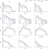 |
Fig. A.1. Distributions of key parameters for SL binary systems from startrack simulations for different SN models and survey instruments, separated by Galactic component (disk and bulge). Parameter distributions include lens mass (Mlens), source mass (Msource), effective Einstein crossing time (τeff), and SL magnification (μsl). Histogram bars with statistically negligible values (𝔼[𝒩SL] ≲ 10−3) for Mlens and Msource are omitted for clarity, and the μsl range is truncated below 10−5 for clarity (cf. fig. 3 in W21). |
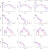 |
Fig. A.2. Parameter distributions for SL binary systems from COSMIC simulations, equivalent to Fig. A.1. |
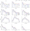 |
Fig. A.3. Parameter distributions for SL binaries with lens masses in the ’mass gap’ region. The plotted lens mass (Mlens) range is restricted to 0–10M⊙ to highlight differences in the mass gap (2–5M⊙). All other aspects are identical to Fig. A.1. |
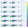 |
Fig. A.5. Relationship between effective Einstein crossing time (τeff) and lens mass (Mlens) across Galactic components, surveys, and SN engine models. The colour-centre scale is consistent across all panels, revealing three distinct populations of SL systems. The mass gap region (Mlens ∈ [2, 5]) shows the highest population density in the f05 model and the lowest in the f40 model. |
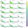 |
Fig. A.6. Relationship between lens mass (Mlens) and centre-of-mass velocity (vcm) across all models. The columns allow comparison between different SN engines, while rows differentiate between surveys (LSST, ZTF, and TESS) and Galactic components (disk and bulge). |
Model predictions showing the number of detectable SL events for different thresholds of coverage (ncov) and recurrence (nrec).
Model predictions for the total number of observations (ntot) of SL events over the full survey duration.
Properties of SL sources broken down by detectability
All Tables
Model predictions showing the number of detectable SL events for different thresholds of coverage (ncov) and recurrence (nrec).
Model predictions for the total number of observations (ntot) of SL events over the full survey duration.
All Figures
|
Fig. 1. Intrinsic mass distribution of Galactic NSs and BHs in binaries with non-compact companions from startrack. Top panel: Bulge sources. Bottom panel: Disk sources. |
| In the text | |
|
Fig. 2. Intrinsic mass distribution of non-compact binary companions in Galactic systems from startrack. Top panel: Bulge sources. Bottom panel: Disk sources. |
| In the text | |
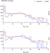 |
Fig. 3. Same as Figure 1, but from COSMIC. |
| In the text | |
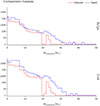 |
Fig. 4. Same as Figure 2, but from COSMIC. |
| In the text | |
|
Fig. 5. Intrinsic mass distribution of Galactic NSs (Mlens < 2.5 M⊙) in binaries with non-compact companions. This shows a focused view of the NS population from Figure 1. |
| In the text | |
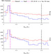 |
Fig. 6. Same as Figure 5 but from COSMIC. |
| In the text | |
|
Fig. 7. Relationship between effective Einstein crossing time (τeff) and lens mass (Mlens) for the Galactic disk population in ZTF observations with f = 4.0. Other models, instruments, and Galactic components are presented in Fig. A.5. |
| In the text | |
|
Fig. 8. Centre-of-mass velocity (vcm) distributions for SL binaries for different SN engines and surveys, separated by Galactic component (disk and bulge). |
| In the text | |
|
Fig. 9. Centre-of-mass velocity (vcm) distributions comparing different surveys (LSST, ZTF, and TESS) for each SN engine and Galactic component. |
| In the text | |
|
Fig. A.1. Distributions of key parameters for SL binary systems from startrack simulations for different SN models and survey instruments, separated by Galactic component (disk and bulge). Parameter distributions include lens mass (Mlens), source mass (Msource), effective Einstein crossing time (τeff), and SL magnification (μsl). Histogram bars with statistically negligible values (𝔼[𝒩SL] ≲ 10−3) for Mlens and Msource are omitted for clarity, and the μsl range is truncated below 10−5 for clarity (cf. fig. 3 in W21). |
| In the text | |
|
Fig. A.2. Parameter distributions for SL binary systems from COSMIC simulations, equivalent to Fig. A.1. |
| In the text | |
|
Fig. A.3. Parameter distributions for SL binaries with lens masses in the ’mass gap’ region. The plotted lens mass (Mlens) range is restricted to 0–10M⊙ to highlight differences in the mass gap (2–5M⊙). All other aspects are identical to Fig. A.1. |
| In the text | |
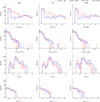 |
Fig. A.4. Equivalent of Fig. A.3 from COSMIC. |
| In the text | |
|
Fig. A.5. Relationship between effective Einstein crossing time (τeff) and lens mass (Mlens) across Galactic components, surveys, and SN engine models. The colour-centre scale is consistent across all panels, revealing three distinct populations of SL systems. The mass gap region (Mlens ∈ [2, 5]) shows the highest population density in the f05 model and the lowest in the f40 model. |
| In the text | |
|
Fig. A.6. Relationship between lens mass (Mlens) and centre-of-mass velocity (vcm) across all models. The columns allow comparison between different SN engines, while rows differentiate between surveys (LSST, ZTF, and TESS) and Galactic components (disk and bulge). |
| In the text | |
Current usage metrics show cumulative count of Article Views (full-text article views including HTML views, PDF and ePub downloads, according to the available data) and Abstracts Views on Vision4Press platform.
Data correspond to usage on the plateform after 2015. The current usage metrics is available 48-96 hours after online publication and is updated daily on week days.
Initial download of the metrics may take a while.