| Issue |
A&A
Volume 706, February 2026
|
|
|---|---|---|
| Article Number | A333 | |
| Number of page(s) | 9 | |
| Section | Galactic structure, stellar clusters and populations | |
| DOI | https://doi.org/10.1051/0004-6361/202557630 | |
| Published online | 23 February 2026 | |
Modeling the formation of ultra-faint dwarf spheroidal galaxies in an extreme collapsing scenario
Simulating Ursa Major II using AMUSE
Departamento de Astronomía, Universidad de Concepción,
Avenida Esteban Iturra s/n,
Concepción,
Chile
★ Corresponding author: This email address is being protected from spambots. You need JavaScript enabled to view it.
Received:
9
October
2025
Accepted:
10
January
2026
Abstract
Context. The ultra-faint dwarf spheroidal galaxies (UFDs) around the Milky Way are the faintest, oldest, and most dark-matter-dominated systems known, providing an unique opportunity to understand early galaxy formation and how dark matter (DM) behaves in the smallest halos. There is an ongoing debate over their formation, despite the several proposed models, they fail to explain UFDs that appear to have evolved in isolation, without external tidal influence.
Aims. To explore the isolated models. We aim to prove if an extreme collapsing scenario could reproduce the size, velocity dispersion, and spherical shape of a classical UFD and to show how it would differ from a virial equilibrium one.
Methods. We considered the dissolving-star-cluster model, adapted to UFDs. Here, the stars are initially distributed in a fractal pattern within the center of the DM halo. Which builds the faint luminous component. We modeled the UFD Ursa Major II, in an initially collapsed formation scenario by performing multiple numerical simulations, using the Astrophysical Multipurpose Software Environment (AMUSE), where the stars follow a fractal distribution within a Plummer DM halo and studying their evolution through 1 Gyr.
Results. The simulations produce a non-spherical object, where the half-mass radius (R50) completely depends on the initial fractal radius. The stability of the object is only reached when the fractal radius is larger than the DM scale length. To reproduce UMa II’s 3D r1/2 ≈ 184 pc, we require an initial fractal radius of ≈ 500 pc. The velocity dispersions are higher than the observed σLOS ≈ 5.6 kms−1, depending on both the fractal and Plummer radii. These results demonstrate that nonequilibrium fractal collapse can reproduce the characteristic size of an UFD without invoking tidal stripping. However, to match the predicted kinematics with observations it may require lowering the mass of the DM halo.
Key words: galaxies: dwarf / galaxies: evolution / galaxies: formation / Local Group
© The Authors 2026
 Open Access article, published by EDP Sciences, under the terms of the Creative Commons Attribution License (https://creativecommons.org/licenses/by/4.0), which permits unrestricted use, distribution, and reproduction in any medium, provided the original work is properly cited.
This article is published in open access under the Subscribe to Open model. This email address is being protected from spambots. You need JavaScript enabled to view it. to support open access publication.
1 Introduction
Dwarf spheroidal galaxies (dSph) are considered the remains of the building blocks of the galaxy-formation process in the Λ-cold-dark-matter (Λ-CDM) model (Assmann et al. 2013b). They have an absolute magnitude ranging from Mv ∼−8.7 to ∼−13.5. Their half-light radii are ≳ 200 pc, and with the exception of Sextans and Ursa Minor, their central surface brightnesses are μ0, V ∼ 22.5−27 mag arcsec−2. Their stellar masses range from M ≈ 105−107 M⊙ (Battaglia et al. 2013; Bullock & Boylan-Kolchin 2017). They are characterized by high dark matter (DM) content, with mass-to-light ratios often reaching ∼ 100 M⊙/L⊙ (Battaglia et al. 2013; Simon 2019).
These galaxies trace their origins to the first billion years after the Big Bang, when DM halos of 107−108 M⊙ collected primordial gas that cooled and fragmented to form stars (Sawala et al. 2009). As the cosmic ultraviolet background intensified during re-ionization (z ≈ 6), photo-heating suppressed further gas accretion in these shallow potential wells, quenching star formation in the smallest halos (Sobacchi & Mesinger 2013).
Following this epoch, three different processes were proposed in order to explain how these objects evolved into the gas-poor spheroid shape that we observe in the Local Group. In the first one, these early dwarfs were trapped by the halos of larger galaxies and effects such as tidal forces, and ram pressure gradually stripped away their gas and stars, leaving behind DM-dominated spheroids, as proven by the Mayer et al. (2007) and D’Onghia et al. (2009) models. In the second case, once ram pressure has removed the galaxy’s gaseous halo, further gas accretion is suppressed, leading to a slow decline in the star-formation rate (SFR). This mode of quenching is commonly referred to as “starvation” or “strangulation” (Balogh et al. 2000; Larson et al. 1980). van de Voort et al. (2017) further showed that satellite galaxies are particularly sensitive to environmental effects, as their gas accretion rates can vary by several orders of magnitude, strongly influencing their ability to sustain star formation. In the third scenario, Sawala et al. (2009) showed that even in isolation, the feedback of supernova outbursts and ultraviolet background could quench star formation, reproducing the dynamical and chemical evolution of the faint systems matching Local Group dwarfs, suggesting that environmental effects were not strictly required.
In addition to isolated scenarios, Assmann et al. (2013b) proposed the dissolving star cluster model, in which the stars formed hierarchically in sub-clusters embedded within a DM halo. The ensuing dissolution of these clusters, due to gas expulsion, produces diffuse stellar distributions and velocity dispersions consistent with observations of classical dSphs. This model introduces a purely internal mechanism capable of shaping dSph structural and kinematic properties, and predicts the presence of kinematic substructures, fossil remnants, of the dissolved clusters. Recently, Alarcón Jara et al. (2023) used kinematic data of Leo 1 to deliver observational evidence that supports this scenario, by identifying substructures in Leo 1 that are consistent with the fossil remnants predicted by Assmann et al. (2013b).
By the early 2010s, due to the digital surveys SDSS and ES/Pan-STARRS, the attention shifted to the newly discovered ultra-faint dwarf galaxies (UFDs), with luminosities of L ≲ 105 L⊙ and metallicities of [Fe/H] ≲−2 (Muñoz et al. 2006; Martin et al. 2007; Simon & Geha 2007). Stellar masses of M ≈ 102−105 M⊙ placed them among the oldest galaxies. With half-light radii as small as ∼ 20 pc and surface brightnesses that can be ∼ 2−3 mag arcsec−2 fainter than that of Sextans (Simon 2019; Bullock & Boylan-Kolchin 2017). Their extreme mass-to-light ratios often exceeding 1000 M⊙/L⊙ and measured velocity dispersions of 5−10 km s−1 revealed DM domination far beyond that of classical dwarfs (Simon & Geha 2007). They no longer present an evolution after the re-ionization epoch and are considered to be pristine relics from the early Universe, providing the opportunity to study the formation of the first galaxies and the behavior of the DM on a small scale (Bovill & Ricotti 2011).
The formation of these faint galaxies is a subject of an ongoing debate. Lokas et al. (2012) revisited tidal stirring for UFDs, finding that highly eccentric orbits could strip stellar mass while preserving high dispersions. Building on the dissolving-cluster model of Assmann et al. (2013b), Aravena et al. (2019) extended it to the UFDs by setting the stars in an initial fractal distribution within a DM halo. Their simulations showed that the gradual dissolution of these fractal sub-clusters could reproduce the faint luminous component and kinematic properties of UFDs, without the need for external tidal stripping.
The observational measures of velocity dispersions of UFDs (5−10 km s−1) far exceed the values expected from their stellar masses, confirming their status as the most dark-matter-dominated systems known (Simon 2019). The use of spectroscopic surveys revealed a wide range of metallicities indicating extended or multiple episodes of star formation and distinguishing UFDs from simple star clusters, which typically exhibit chemically homogeneous populations (Simon & Geha 2007; Kirby et al. 2013). These results, despite providing a better understanding of these galaxies, also expose unresolved theoretical problems. One is the difference between the steep central density cusps predicted by Λ CDM simulations, and the flatter, core-like profiles inferred from stellar kinematics; this is known as the core-cusp problem (Navarro et al. 1996; Peñarrubia et al. 2008; de Blok 2010). We note, however, that UFDs contain too few stars to measure reliable radial-velocity gradients, and current discussions of core-cusp structure in these systems are based primarily on their radial density profiles rather than on spatially resolved kinematics (Sánchez Almeida et al. 2024). Although our model does not attempt to address this issue directly, it provides a reference point to explore how nonequilibrium stellar dynamics within a static halo might influence the interpretation of internal velocity–dispersion profiles.
In this work, we considered the formation scenario for UFD proposed by Aravena et al. (2019), consisting of an initial fractal distribution for the stellar component of the galaxy (Goodwin & Whitworth 2004), within a DM halo following a Plummer potential. It is not intended to represent the expected Λ CDM density profile of UMa II by the use of this potential. It is instead a methodological choice. A cored potential provides a smooth, finite central acceleration that avoids numerical divergences during the extreme early phase, unlike the virial-equilibrium-based models used before. We explored a non-virial collapse scenario.
Specifically, we initialized stars at zero velocity and followed their evolution over 1 Gyr. This allowed us to isolate the stellar dynamical evolution independently of the detailed DM distribution. This also ensures consistency with previous work exploring the same formation scenario (Aravena et al. 2019). Our goal is to test whether such a collapsing fractal model can evolve into the observed half-light radii, velocity dispersions, and stellar morphology of systems such as the UFD UMa II.
2 Methodology
Similarly to the methodology followed by Aravena et al. (2019), we performed our simulations using the Astrophysical Multipurpose Software Environment (AMUSE; Pelupessy et al. 2013; Portegies Zwart & McMillan 2018).
2.1 AMUSE
It is a Python-based software designed to unify different astrophysical codes in one interface. For our gravitational N-body simulations, we considered the ph4 integrator, a fourth-order Hermite scheme optimized for GPU acceleration and individual time steps (Makino & Aarseth 1992).
To represent the fixed background potential of the DM halo, we used the Bridge method (Fujii et al. 2008), which allows a live N-body stellar component to evolve under the influence of an analytic potential. Additionally, we enabled the multiples module in AMUSE to properly handle close stellar encounters. During collapse, especially in the early stages when the system is far from equilibrium, some particles can approach each other very closely, which can lead to inaccurate force calculations if not treated in detail (Portegies Zwart & McMillan 2018). To correct these possible false data, when two or more stars come within a critical distance based on their relative velocity and total mass the code identifies them as a subsystem and temporarily switches to a high-accuracy, few-body integrator to follow their motion. This prevents numerical instabilities and helps conserve energy during strong interactions (Binney & Tremaine 2008, p 581). The encounter condition is set roughly by
 (1)
This approach is particularly important in our case, since we started with all stars having zero velocity, leading to a strong central collapse.
(1)
This approach is particularly important in our case, since we started with all stars having zero velocity, leading to a strong central collapse.
2.2 Ursa Major II
As a fiducial model for our scenario, we considered the UFD Ursa Major II (UMa II), one of the faintest known satellites of the Milky Way, with an absolute magnitude of Mv ≈−3.6 mag, a half-light radius of r1/2 ≈ 140 pc, a 3D r1/2 ≈ 184 pc, and a dynamical mass within that radius of M1/2 ≈ 7.9 × 10⁶ M⊙, implying a mass-to-light ratio of M/Lv ∼ 2000 M⊙/L⊙ and indicating a strong dominance of DM (Zucker et al. 2006; Simon & Geha 2007; Wolf et al. 2010). We used these observational properties as reference points to set the structural and dynamical parameters in our simulations.
Observational constraints suggest that UMa II may also be undergoing tidal disruption, based on its distorted morphology and velocity gradients (Simon & Geha 2007). This cannot be taken into account in our simulations as we made UMa II in isolation. The combination of extreme faintness, large velocity dispersion, and low surface brightness makes it an ideal test case for models of early galaxy formation and internal stellar dynamics.
Summary of the initial conditions of the stars.
2.3 DM halo
The DM halo is modeled using an analytical background density. In this case, we used a cored Plummer potential (Plummer 1911),
 (2)
which can be derived by the Poisson equation into the density distribution (Binney & Tremaine 2008, 230):
(2)
which can be derived by the Poisson equation into the density distribution (Binney & Tremaine 2008, 230):
 (3)
We adopted a Plummer radius of RPl = 50, 100, 250, 500 pc and determined the corresponding total mass MPl required to reproduce the observed mass enclosed within r1/2=140 pc using
(3)
We adopted a Plummer radius of RPl = 50, 100, 250, 500 pc and determined the corresponding total mass MPl required to reproduce the observed mass enclosed within r1/2=140 pc using
 (4)
The Plummer masses obtained by replacing the dynamical mass within the half-light radius of UMa II in Eq. (4) are summarized in Table 1.
(4)
The Plummer masses obtained by replacing the dynamical mass within the half-light radius of UMa II in Eq. (4) are summarized in Table 1.
2.4 Initial conditions
We initially set the stellar component as a fractal distribution, following the method described by Goodwin & Whitworth (2004) and followed by Aravena et al. (2019). Fractal initial conditions are commonly used to mimic the clumpy, hierarchically clustered nature of star-forming regions, where stars form in sub-structured associations rather than in smooth spherical profiles. This approach has been shown to produce realistic early dynamical evolution in systems undergoing collapse (Aravena et al. 2019; Goodwin & Whitworth 2004). The process starts with a cube that is divided into  sub-cubes, in our case
  , and only a fraction of them were randomly selected based on the fractal dimension, D. We considered D= 1.6, which lies in the range measured for star-forming clouds and young stellar groups, typically D ∼ 1.4−2.0 (Goodwin & Whitworth 2004), and produces a clumpy, spatially correlated distribution consistent with the highly irregular morphology expected in the early stages of UFD formation. This selection is repeated until the target number of particles is reached, and the resulting structure is then scaled to the chosen fractal radius, rfrac, and centered at the origin (Goodwin & Whitworth 2004).
The final system has 4000 equal-mass particles, each with M*=0.5 M⊙, giving a total stellar mass of Mtot=2000 M⊙. All the parameters used to build the initial conditions including the fractal and halo properties are listed in Table 1.
The main difference with previous studies (Aravena et al. 2019; Cabello-Cabello et al. 2024) is that in here, we started with a system where all particles are at rest, i.e., with the virial ratio set as α=0, where α=2T/|W| measures the degree of kinetic support against self-gravity; thus, the evolution is expected to be driven entirely by gravitational collapse. We tested five different values for the initial fractal radius: rfrac = 50, 100, 200, 400, 500 pc, combined with four different Plummer radii for the dark halo. For each combination, we ran five realizations with different random seeds in order to study how much the structure of the initial and final distribution could vary. Some examples of these different initial setups are shown in the top row of Fig. 1. Despite the fact that all the input parameters are the same, the internal structure and clumping change from one realization to another, simply because of the random seed in the fractal generator.
To quantify the statistical properties of the initial conditions and evaluate how much the internal substructure varies between realizations, we analyzed the 3D radial mass-density profile, ρ(r), at t=0 for each run. The profiles were obtained by binning the particle distribution in spherical shells and converting the number of particles in each shell into a mass density, considering equal particle masses. Figure 2 shows the mean density profile obtained by averaging the realizations for a representative case (rfrac = 100 pc), and the shaded region indicates the variance. The resulting initial half-mass radius is R50 = 52.2 pc for this configuration. At small radii, the dispersion between realizations is intrinsically low, because the fractal algorithm generates a strong central concentration; on the other hand, at larger radii the variance increases due to stochastic fluctuations in hierarchical structure (Goodwin & Whitworth 2004; Allison et al. 2010). The value of the initial R50 provides a robust characterization of the initial scale of the system and will be compared with the final half-mass radius.
3 Results
Following the five realizations during 1 Gyr of each set of parameters, the evolution of the galaxy showed a similar initial pattern in every iteration.
3.1 Evolution of the galaxy
In this work, we adopted a dynamical definition of virial equilibrium for the stellar component, understood as a quasi-stationary state in which the virial equation is approximately satisfied. Following Terebizh (2024), the virial equation for a system of N gravitating particles can be written in the center-of-mass frame by the Lagrange–Jacobi identity:
 (5)
where J(t) is the moment of inertia, K(t) is the total kinetic energy, and W(t) the gravitational potential energy. For stellar systems, which are not spatially closed, the virial theorem does not hold instantaneously. However, it is commonly assumed that after sufficient evolution the system approaches a quasistationary state, in which the second time derivative of the moment of inertia becomes small compared to the other terms.
(5)
where J(t) is the moment of inertia, K(t) is the total kinetic energy, and W(t) the gravitational potential energy. For stellar systems, which are not spatially closed, the virial theorem does not hold instantaneously. However, it is commonly assumed that after sufficient evolution the system approaches a quasistationary state, in which the second time derivative of the moment of inertia becomes small compared to the other terms.
In this regime, averaging the virial equation over time yields
 (6)
which defines the virial equilibrium state (VES) in the sense discussed by Terebizh (2024).
(6)
which defines the virial equilibrium state (VES) in the sense discussed by Terebizh (2024).
In the presence of a dominant external potential, the potential energy must include the interaction between the stars and the external field, so the virial balance refers to the luminous component embedded in the halo. In this framework, relaxation toward equilibrium occurs over a timescale of a few tens of dynamical (crossing) times, after which point global parameters such as the half-mass radius and virial ratio stabilize (Terebizh 2024). The persistent oscillations in the R50 indicate that the stellar component has not yet settled into the quasi-virial equilibrium
Although we have galaxies with fractal and Plummer radii ranging from 50 pc to 500 pc, every set of parameter shares the initial collapse. As an example of this behavior, we can consider Fig. 3. To analyze if 1 Gyr is sufficient to characterize the long-term evolution of the system, we tried a simulation with RPl=500 pc and rfrac = 500 pc for 5 Gyr. At the first 50 Myr the particles move toward the center due to gravitational collapse, then a cycle of collapsing and expanding stellar distribution begins, which seems to become stable at 500 Myr. However, at 1, 3, and 5 Gyr particles are still passing through the center.
The nature of a non-virial equilibrium system led us to expect this scenario. The choice of 1 Gyr is not intended to ensure virial equilibrium, but to move beyond the initial collapse phase and characterize the system at late times. The final shape of the object does not seem to reassemble the classical dSph, but after 1 Gyr the galaxy will slowly assume its final shape.
To understand the odd shape of these galaxies, we considered the different realizations of the exact same set of parameters of the Fig. 1: RPl=250 pc and rfrac = 100 pc. In the bottom row of Fig. 1, after 1 Gyr of evolution, the shape of each one is completely different. As the only difference is the random seed of the fractal generator, it is safe to conclude that the final shape of the galaxy will only depend on the initial distribution of the particles.
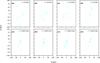 |
Fig. 1 Top row: Examples of stars’ initial fractal distributions (t=0 Gyr) for four of the five realizations, with a fractal radius of rfrac = 100 pc, Plummer radius of PPl=250 pc, and MPl=6.9 × 10⁷ M⊙, respectively. Panels (a), (b), (c), and (d) have the exact same parameters; the only difference is the random seed for the fractal generator. Bottom row: End of evolution (t=1 Gyr) of the 4000 particles. Panels (a′), (b′), (c′), and (d’) represent the end of the evolution (t=1 Gyr) of (a), (b), (c), and (d), respectively. |
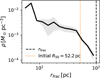 |
Fig. 2 Initial 3D radial mass-density profile for five realizations with identical physical parameters (rfrac = 100 pc), but with a random seed. The solid black line shows the mean density profile, and the shaded region indicates the variance between realizations. The initial half-mass radius is R50=52.2 pc. At larger radii, the dispersion increases. |
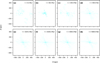 |
Fig. 3 Evolution of 4000 particles distributed as initial fractal pattern of rfrac = 500 pc, MPl=4 × 10⁸ M⊙, within an analytical DM halo of RPl=500 pc. The initial velocity of these particles is 0 kms−1. Panels (a), (b), (c), (d), (e), (f), (g), and (h) represent the time steps from 0 to 5 Gyr. |
3.2 Size of the galaxy
To estimate the radius of the galaxy, we measured Lagrangian radii, i.e., the radius of an imaginary sphere at the center of a stellar system containing a fixed proportion of its mass (Sweatman 1993). Specifically, we considered the Lagrangian radius at 50% after 1 Gyr of evolution as a function of the Plummer radius. To compute the Lagrangian radii, we adopted the center of the total gravitational potential as the reference point. Since the stellar component evolves inside a fixed, spherically symmetric Plummer halo, the minimum of the potential is well defined and coincides with the coordinate origin at all times.
We focused on R50 because the 3D half-mass radius is comparable to the 3D half-light radius measured in Local Group UFDs under the standard assumption of a radially uniform stellar mass-to-light ratio, appropriate for old, single-age populations (Wolf et al. 2010; McConnachie 2012). While observed values refer to the projected distribution, the conversion between 2D half-light and 3D half-light radii is well defined in equilibrium systems (Wolf et al. 2010). Moreover, R50 provides a robust global scale that traces the main dynamical evolution of the system, while reducing the influence of the outer regions, with low particle counts in initial fractal distribution, which lead to large statistical noise. To identify if this parameter is sufficient to capture the overall structure of the stellar component, we analyzed the projected radial surface density profile of the final system. Figure 4 shows the normalized surface-density profile of a representative model compared to a Plummer profile with scale radius set by the final R50. Despite differences in their dynamical state, the simulated stellar systems develop a surface density consistent with those commonly adopted to describe UFDs.
Compared with the initial configuration of Fig. 2 (R50= 52.2 pc), the system undergoes a substantial contraction of its half-mass radius to a value of R50 ≈ 31 pc (Table 2), driven by gravitational collapse from the initially sub-structured fractal state.
Figure 5 illustrates that the system does not always reach a stable structure by the end of the simulation. Panel (a) shows the evolution of the half-mass radius for a fractal radius of rfrac = 50 pc compared to the different scale length of the DM halo. The half-mass radius typically stabilizes from R50 ∼ 15− 20 pc depending on the RPl. If we consider RPl=50 pc, the object will become stable within the first 100 Myr. However, for RPl=500 pc, the galaxy seems to be oscillating during the whole simulation. This effect is produced by the fact that the inner region of a Plummer halo is approximately harmonic, the stellar orbits undergo quasi-periodic oscillations around the equilibrium structure (Binney & Tremaine 2008, Ch. 2.2; Ch. 3.1).
Figure 5b also presents a half-mass radius compared to the different scale length of the DM halo, but for a fractal radius of rfrac=500 pc. The half-mass radius will oscillate from R50 ∼ 150−200 pc, also depending on the DM scale length, but this time the galaxy stabilizes at t<200 Myr for every Plummer radius considered. The faster convergence is driven by the shorter dynamical times and stronger gravitational gradients in the inner regions of the halo potential. In a concentrated background potential, collisionless relaxation operates over only a few crossing times and efficiently suppresses the global oscillations of the stellar distribution, which leads to dynamical relaxation, allowing the system to settle into a stable configuration within the simulation time (Binney & Tremaine 2008, Ch. 1.2; Ch. 4.1; Ch. 4.10).
From these two plots, we can observe that evolution and the stability of the galaxy depend on the Plummer radius and how large it is compared to the fractal radius. If we have a DM-halo scale length larger than the fractal radius, we obtain an unstable object, at least during the first gigayear. In the other scenario, we obtain a stable galaxy that slightly oscillates.
To calculate the final R50 of our galaxy, we considered the value at 1 Gyr, which corresponds to ≳ 20 dynamical times for a classical UFD. The initial transient collapse ends within ≲ 200 Myr (Fig. 5), after which the evolution of R50 becomes slow and the system approaches a long-term configuration despite not reaching strict virial equilibrium. Extending the integration time does not significantly change the global parameters (Fig. 3), and therefore 1 Gyr captures the relevant post-collapse structure. In most of the simulations, it matches the mean R50 over the entire evolution. In the few cases where 1 Gyr is not sufficient for the system to reach stability (panel a in Fig. 5, for RPl larger than rfrac), we computed the mean values of R50 every 200 Myr over 1 Gyr, the errors are computed as the standard deviation of the mean values across five realizations. The resulting R50 values are listed in Table 2.
Figure 6 shows the direct dependence of the final half-mass radius as a function of the initial fractal radius for each fixed Plummer radius. At larger fractal distributions, we obtain larger half-mass radii, but also bigger error bars. On the other hand, the dependency on the Plummer radius seems nonexistent, although there are exceptions; for example, at rfrac=500 pc the Plummer radius of RPl=250 pc gives a half-mass radius value closer to the observations than the others tested at the same fractal scale. In the collapsing scenario, we can conclude that the dependency of the half-mass radius is almost entirely on the fractal radius, and, as a result, measuring the half-light radius of a UFD would have no relation with the underlying DM-halo distribution of mass.
In simulations with rfrac<350 pc, the obtained half-mass radius does not resemble that of the observational data; hence, they result in galaxies that are smaller than intended. Meanwhile, at rfrac>450 we obtain R50 ∼ 180 pc, but the dispersion between realizations is too large to obtain reliable results. To reproduce UMa II 3D r1/2, we would need an initial fractal radius in between rfrac ∼ 400 and 500 pc, as marked in gray in Fig. 6. From our simulations, the closest value is given by rfrac=500 pc.
Summary of model parameters and resulting quantities.
 |
Fig. 4 Normalized projected stellar surface density profile, Σ(R), of the simulated system at the final snapshot for a model with RPl=500 pc and rfrac = 100 pc. The solid black line shows the normalized surface density obtained from the simulation after projecting the normalization on the x−z plane. The dashed red line corresponds to a normalized projected Plummer profile with the same scale radius, shown for reference. No observational surface density profile is available for UMa II; therefore, the comparison is restricted to idealized models. The deviations from a Plummer profile indicate that this functional form does not provide an optimal description of the final stellar distribution in our simulations. |
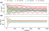 |
Fig. 5 Lagrangian radii at 50% (radius containing half of the mass: R50[pc]) compared to evolution of simulation t=1 Gyr. Each curve shows the mean over five realizations per time step; the associated standard deviations are not shown, for visual clarity, but the last time steps are reported in Table 2. For panel (a), we considered a fractal radius of rfrac=50 pc. In the case of panel (b), we used rfrac=500 pc. The colored figures represent the Plummer radii RPl=50, 100, 250, 500 pc. |
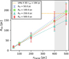 |
Fig. 6 Half-mass radius compared with initial fractal scale length for each Plummer radius. The colored figures represent the RPl = 50, 100, 250, and 500 pc. The colored dotted lines set the fit for each RPl. The dotted horizontal yellow line is the 3D half-light radius of UMa II (Wolf et al. 2010). The vertical gray rectangle represents the range of rfrac in which the UMa 3D r1/2 can be reached. Data obtained from Table 2. |
3.3 Velocity dispersion
To determine the standard deviation for the mean velocity of the particles within the system, we used the 1D velocity-dispersion σ. We considered all stars within the half-mass radius and measured the line-of-sight (LOS) dispersion along each coordinate axis separately. The mean values with their respective errors are summarized in Table 2.
The observed LOS velocity dispersion in UMa II is derived from kinematic samples that include all detected member stars projected along the LOS, extending beyond the half-light radius (Wolf et al. 2010). In our model, values were computed by selecting stars within the half-mass radius R50. This excludes contributions from stars at larger projected radii, where loosely bound stars, tidal features, or ongoing oscillations can increase the measured velocity dispersion. Therefore, our measurements may represent a lower limit to the true LOS velocity dispersion of our simulations.
Figure 7 represents the LOS along the y-axis, as Table 2 shows that the values along the three coordinate axes are similar within their large error-bars. The dotted orange line represents the measured dispersion of UMa II with the shaded area denoting the 1−σ uncertainty. We see that even under the assumption of a lower limit for σLOS, our simulations show an agreement with the observed value at small fractal sizes (50−200 pc), while we see in Fig. 6 that only larger fractal sizes can reproduce the observed half-mass radius; i.e., we cannot reproduce size and velocity dispersion of UMa II simultaneously with our models. Including stars beyond R50 would likely increase the measured σLOS in our simulations, further widening the discrepancy between size and velocity dispersion. Therefore, the mismatch between the two observables is robust with respect to the choice of aperture for the LOS measurement.
Even though error bars are large, there is a visible trend that with small DM halo scale lengths the velocity dispersion increases more slowly, or even levels off to an almost constant value with increasing the size of the fractal. Large DM halo scales show a linear rise of dispersion with the size of the fractal instead.
This behavior might have two causes. First of all, as σ ∝ M/r, we have more DM mass centrally concentrated and influencing the velocity dispersion at small halo scale lengths. Smaller fractal sizes produce smaller luminous components, but there are higher dispersions at more concentrated halos. Second, as Fig. 5 shows, we see large oscillations around the final size of our luminous component at smaller sizes of the fractal. In the framework described in Sect. 2.4, these persistent oscillations in R50 indicate that the moment of inertia of the stellar component is still evolving in time, which means that the system has not yet reached a quasi-stationary virial state; i.e., our luminous component has not yet reached a virial equilibrium and therefore could show an inflated value, when measuring the velocity dispersion.
This effect is largest if the scale length of the DM halo is large, i.e., much larger that the size of the luminous object (Rpl=500 pc). Here, the DM background density is more or less constant inside the forming object, and we have a more or less harmonic oscillation of stars, leading to a quasi-constant oscillation of the half-mass radius of the formed stellar object. In our framework (Sect. 3.3), virial equilibrium requires a stationary half-mass radius; however, the large oscillations of R50 in Fig. 5 imply d2J/dt2 ≠ 0; i.e., the virial condition is not satisfied. As a result, the measured velocity dispersions include kinetic energy from the radial oscillations and are therefore higher than the equilibrium value.
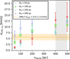 |
Fig. 7 LOS of velocity dispersion of y-axis as function of the initial fractal radius for different Plummer radii. The different figures and colors represent the Plummer radii. The vertical gray rectangle represents the range rfrac ∼ 400−500 pc, where we could represent the 3D half-light radius of UMa II. The dotted yellow line is the observational σLOS=5.6 ± 1.5 km s−1 (Simon 2019). |
4 Discussion and conclusions
We adopted the dissolving star-cluster scenario proposed by Assmann et al. (2013a,b) and altered it to make it applicable to the range of faint and ultra-faint dSph galaxies. The idea is that instead of clusters and associations of forming stars in a large DM halo, we have a single star-forming region in the center of a small DM halo, forming stars in a fractal distribution. Aravena et al. (2019) already showed that such fractal distributions form luminous objects similar to the observed dwarf galaxies.
This study focused on reproducing one particular faint dSph galaxy, namely UMa II, and represents a complementary study to Cabello-Cabello et al. (in prep.). They use similar initial conditions to our study, but give the newly formed stars’ velocities according to virial equilibrium values. We, on the other hand, studied the same formation scenario in the extreme case that all stars are born with zero initial velocities, leading to a strong collapse of the stellar component at the start of each simulation.
In Fig. 8, we compare the results of both scenarios. The data from the equilibrium simulations were taken from the preliminary results from Cabello-Cabello et al. (2024) presented at the XIX SOCHIAS meeting (available on Zenodo). We show the final half-mass radius of the resulting object at the end of our simulation as a function of the scale length of the underlying DM halo. In both studies, cored DM profiles, i.e., Plummer spheres, were used to represent the DM. The initial size of the fractal distribution is represented by the color-coding of the data points. The difference in the results is immediately visible. As explained above, in our study the size of the final object almost completely depends on the initial size of the fractal distribution of the stars and not on the sale length of the DM halo. This behavior is opposite to that of the equilibrium models. There, the results of the simulations suggest that the size of the luminous component only depends on the scale length of the DM halo and is almost independent of the initial size of the stellar distribution.
Both scenarios are extreme cases, and the reality might be somewhere in between. Anyway, it is possible to reproduce the size of UMa II with both scenarios. In our case, we have the difficulty of matching size and velocity dispersion with the same initial values. The large fractal sizes we need to reproduce the size of UMa II lead to velocity dispersions that are about twice the observed value of σLOS=5.6 ± 1.4 kms−1 (Simon 2019). We can partly explain this discrepancy by the notion that our final objects have not yet reached complete virial equilibrium, but they still have adequate harmonic oscillations in terms of size, thereby inflating any measurement of the velocity dispersion and henceforth overestimating the background DM mass.
Observed velocity dispersions are derived under the assumptions of spherical symmetry, isotropy, and virial equilibrium (Simon & Geha 2007; Wolf et al. 2010). If, as in our simulations, the stellar distribution is not in equilibrium (Sect. 2.4), the inferred dynamical mass for the DM halo could be significantly overestimated (El-Badry et al. 2017).
A major shortfall of our study is that we only used cored DM halo profiles. It is up to future studies of our formation scenario to investigate whether some of our obvious problems can be in part healed by using a cusped profile for the DM halo. We expect that at least part of the size oscillations of our objects will be damped by a profile with a density gradient instead of an equal density harmonic profile, as present in our large DM scale-length simulations. In the simulations using equilibrium velocities, the resulting objects are smoother, i.e., there are fewer remaining clumps, spurs or spikes, as shown by (Cabello-Cabello et al. 2024), who in their first results found no significant difference between cored and cusped halo profiles.
Alarcón Jara et al. (2023) showed that the dissolving starcluster Scenario is in accordance with observational data derived from Leo I, a classical dSph galaxy and therefore a valid formation scenario. In fact, it explains the observed data better than models using tidal forces to produce a small dSph galaxy.
In their initial study, Aravena et al. (2019) showed that the extension of the dissolving star-cluster scenario to smaller and fainter dSph galaxies works. We now present the first detailed study of this scenario. We see that even in the extreme velocity case used in this study, we are able to obtain bound stellar systems with sizes comparable to faint dSph galaxies. Using observationally derived parameters to restrict our study to the particular case of Ursa Major II, we were able to reproduce the observed size of UMa II by starting with a fractal stellar distribution of around 500 pc in size, which is would represent a rather large star-forming region. Contrary to a similar study (Cabello-Cabello et al. 2024), we were not able to match the observed velocity dispersion of UMa II with the same initial values needed to match the size.
If the velocities of the initially forming stars are close to zero, leading to an initial collapse, we state that the size of the resulting final luminous object depends almost completely on the initial size of the stellar distribution and is almost independent of the scale length of the DM halo.
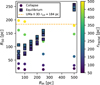 |
Fig. 8 Half-mass radius compared with DM-halo scale length (Plummer radius) for each fractal radius. The circular dots represent the initial collapse scenario, while the square ones describe the behavior of the half-mass radius in the equilibrium scenario. The UMa II 3D half-light radius is represented by the dotted yellow line. Due to the variety of fractal radii, a color gradient is used to represent it. Error bars are omitted. |
References
- Alarcón Jara, A. G., Fellhauer, M., Simon, J., et al. 2023, A&A, 672, A29 [NASA ADS] [CrossRef] [EDP Sciences] [Google Scholar]
- Allison, R. J., Goodwin, S. P., Parker, R. J., Portegies Zwart, S. F., & de Grijs, R., 2010, MNRAS, 407, 1098 [NASA ADS] [CrossRef] [Google Scholar]
- Aravena, C., Fellhauer, M., Urrutia Zapata, F., & Alarcón Jara, A., 2019, BAAA, 61a, 181 [Google Scholar]
- Assmann, P., Fellhauer, M., Wilkinson, M., Smith, R., & Blaña, M., 2013a, MNRAS, 1 [Google Scholar]
- Assmann, P., Fellhauer, M., Wilkinson, M. I., & Smith, R., 2013b, MNRAS, 432, 274 [NASA ADS] [CrossRef] [Google Scholar]
- Balogh, M. L., Navarro, J. F., & Morris, S. L., 2000, ApJ, 540, 113 [Google Scholar]
- Battaglia, G., Helmi, A., & Breddels, M., 2013, New A Rev., 57, 52 [Google Scholar]
- Binney, J., & Tremaine, S., 2008, Galactic Dynamics, 2nd edn. Princeton Series in Astrophysics, 208 [Google Scholar]
- Bovill, M. S., & Ricotti, M., 2011, ApJ, 741, 17 [NASA ADS] [CrossRef] [Google Scholar]
- Bullock, J. S., & Boylan-Kolchin, M., 2017, ARA&A, 55, 343 [Google Scholar]
- Cabello-Cabello, J. A., Fellhauer, M., Matus-Carrillo, D. R., & Vergara-Landeros, J. I., 2024, https://doi.org/10.5281/zenodo.14213118 [Google Scholar]
- de Blok, W., 2010, Adv. Astron., 2010, 789293 [Google Scholar]
- D’Onghia, E., Besla, G., Cox, T. J., & Hernquist, L., 2009, Nature, 460, 605 [CrossRef] [Google Scholar]
- El-Badry, K., Wetzel, A. R., Geha, M., et al. 2017, ApJ, 835, 193 [NASA ADS] [CrossRef] [Google Scholar]
- Fujii, M., Iwasawa, M., Funato, Y., & Makino, J., 2008, ApJ, 686, 1082 [NASA ADS] [CrossRef] [Google Scholar]
- Goodwin, S. P., & Whitworth, A. P., 2004, A&A, 413, 929 [NASA ADS] [CrossRef] [EDP Sciences] [Google Scholar]
- Kirby, E. N., Cohen, J. G., Guhathakurta, P., et al. 2013, ApJ, 779, L107 [Google Scholar]
- Larson, R. B., Tinsley, B. M., & Caldwell, C. N., 1980, ApJ, 237, 692 [Google Scholar]
- Lokas, E. L., Kazantzidis, S., & Mayer, L., 2012, ApJ, 751, L15 [Google Scholar]
- Makino, J., & Aarseth, S. J., 1992, PASJ, 44, 141 [NASA ADS] [Google Scholar]
- Martin, N. F., Ibata, R. A., Chapman, S. C., Irwin, M., & Lewis, G. F., 2007, MNRAS, 380, 281 [CrossRef] [Google Scholar]
- Mayer, L., Kazantzidis, S., Mastropietro, C., & Wadsley, J., 2007, Nature, 445, L738 [Google Scholar]
- McConnachie, A. W., 2012, AJ, 144, 4 [Google Scholar]
- Muñoz, R. R., Carlin, J. L., Frinchaboy, P. M., et al. 2006, ApJ, 650, L51 [CrossRef] [Google Scholar]
- Navarro, J. F., Frenk, C. S., & White, S. D. M., 1996, ApJ, 462, 563 [Google Scholar]
- Pelupessy, F., van Elteren, A., de Vries, N., et al. 2013, A&A, A84 [NASA ADS] [CrossRef] [EDP Sciences] [Google Scholar]
- Peñarrubia, J., Navarro, J. F., & McConnachie, A. W., 2008, Astron. Nachr., 329, 934 [Google Scholar]
- Plummer, H. C., 1911, MNRAS, 71, 460 [Google Scholar]
- Portegies Zwart, S., & McMillan, S., 2018, Astrophysical Recipes The art of AMUSE (IOP Publishing) [Google Scholar]
- Sánchez Almeida, J., Trujillo, I., & Plastino, A. R. 2024, ApJ, 973, L15 [Google Scholar]
- Sawala, T., Scannapieco, C., Maio, U., & White, S. D., 2009, MNRAS, 402, 1599 [Google Scholar]
- Simon, J., 2019, ARA&A, 57, 375 [Google Scholar]
- Simon, J. D., & Geha, M., 2007, ApJ, 670, 313 [NASA ADS] [CrossRef] [Google Scholar]
- Sobacchi, E., & Mesinger, A., 2013, MNRAS, 672, L40 [Google Scholar]
- Sweatman, W. L., 1993, MNRAS, 261, 497 [Google Scholar]
- Terebizh, V. Y., 2024, A&A, 686, A35 [NASA ADS] [CrossRef] [EDP Sciences] [Google Scholar]
- van de Voort, F., Bahé, Y. M., Bower, R. G., et al. 2017, MNRAS, 466, 3460 [NASA ADS] [CrossRef] [Google Scholar]
- Wolf, J., Martinez, G. D., Bullock, J. S., et al. 2010, MNRAS, 406, 1220 [NASA ADS] [Google Scholar]
- Zucker, D. B., Belokurov, V., Evans, N. W., et al. 2006, ApJ, 650, L41 [Google Scholar]
All Tables
All Figures
|
Fig. 1 Top row: Examples of stars’ initial fractal distributions (t=0 Gyr) for four of the five realizations, with a fractal radius of rfrac = 100 pc, Plummer radius of PPl=250 pc, and MPl=6.9 × 10⁷ M⊙, respectively. Panels (a), (b), (c), and (d) have the exact same parameters; the only difference is the random seed for the fractal generator. Bottom row: End of evolution (t=1 Gyr) of the 4000 particles. Panels (a′), (b′), (c′), and (d’) represent the end of the evolution (t=1 Gyr) of (a), (b), (c), and (d), respectively. |
| In the text | |
|
Fig. 2 Initial 3D radial mass-density profile for five realizations with identical physical parameters (rfrac = 100 pc), but with a random seed. The solid black line shows the mean density profile, and the shaded region indicates the variance between realizations. The initial half-mass radius is R50=52.2 pc. At larger radii, the dispersion increases. |
| In the text | |
|
Fig. 3 Evolution of 4000 particles distributed as initial fractal pattern of rfrac = 500 pc, MPl=4 × 10⁸ M⊙, within an analytical DM halo of RPl=500 pc. The initial velocity of these particles is 0 kms−1. Panels (a), (b), (c), (d), (e), (f), (g), and (h) represent the time steps from 0 to 5 Gyr. |
| In the text | |
|
Fig. 4 Normalized projected stellar surface density profile, Σ(R), of the simulated system at the final snapshot for a model with RPl=500 pc and rfrac = 100 pc. The solid black line shows the normalized surface density obtained from the simulation after projecting the normalization on the x−z plane. The dashed red line corresponds to a normalized projected Plummer profile with the same scale radius, shown for reference. No observational surface density profile is available for UMa II; therefore, the comparison is restricted to idealized models. The deviations from a Plummer profile indicate that this functional form does not provide an optimal description of the final stellar distribution in our simulations. |
| In the text | |
|
Fig. 5 Lagrangian radii at 50% (radius containing half of the mass: R50[pc]) compared to evolution of simulation t=1 Gyr. Each curve shows the mean over five realizations per time step; the associated standard deviations are not shown, for visual clarity, but the last time steps are reported in Table 2. For panel (a), we considered a fractal radius of rfrac=50 pc. In the case of panel (b), we used rfrac=500 pc. The colored figures represent the Plummer radii RPl=50, 100, 250, 500 pc. |
| In the text | |
|
Fig. 6 Half-mass radius compared with initial fractal scale length for each Plummer radius. The colored figures represent the RPl = 50, 100, 250, and 500 pc. The colored dotted lines set the fit for each RPl. The dotted horizontal yellow line is the 3D half-light radius of UMa II (Wolf et al. 2010). The vertical gray rectangle represents the range of rfrac in which the UMa 3D r1/2 can be reached. Data obtained from Table 2. |
| In the text | |
|
Fig. 7 LOS of velocity dispersion of y-axis as function of the initial fractal radius for different Plummer radii. The different figures and colors represent the Plummer radii. The vertical gray rectangle represents the range rfrac ∼ 400−500 pc, where we could represent the 3D half-light radius of UMa II. The dotted yellow line is the observational σLOS=5.6 ± 1.5 km s−1 (Simon 2019). |
| In the text | |
|
Fig. 8 Half-mass radius compared with DM-halo scale length (Plummer radius) for each fractal radius. The circular dots represent the initial collapse scenario, while the square ones describe the behavior of the half-mass radius in the equilibrium scenario. The UMa II 3D half-light radius is represented by the dotted yellow line. Due to the variety of fractal radii, a color gradient is used to represent it. Error bars are omitted. |
| In the text | |
Current usage metrics show cumulative count of Article Views (full-text article views including HTML views, PDF and ePub downloads, according to the available data) and Abstracts Views on Vision4Press platform.
Data correspond to usage on the plateform after 2015. The current usage metrics is available 48-96 hours after online publication and is updated daily on week days.
Initial download of the metrics may take a while.