| Issue |
A&A
Volume 706, February 2026
|
|
|---|---|---|
| Article Number | A366 | |
| Number of page(s) | 11 | |
| Section | Extragalactic astronomy | |
| DOI | https://doi.org/10.1051/0004-6361/202557635 | |
| Published online | 20 February 2026 | |
Not so Swift: 20 years of multi-wavelength observations of Mrk 421 and Mrk 501
1
Landessternwarte, Universität Heidelberg Königstuhl D-69117 Heidelberg, Germany
2
Institute of Nuclear Physics, Polish Academy of Sciences PL-31342 Krakow, Poland
3
Centre for Space Research, North-West University Potchefstroom 2520, South Africa
★ Corresponding author: This email address is being protected from spambots. You need JavaScript enabled to view it.
Received:
10
October
2025
Accepted:
7
January
2026
Abstract
Aims. The blazars Mrk 421 and Mrk 501 have shown multi-wavelength variability on all observed timescales, and have been well studied at high energies on short timescales. We aim to characterise the long-term temporal behaviour of these blazars at synchrotron energies, namely in the optical, UV, and X-ray, in order to assess current models of these objects and their processes.
Methods. Including amongst the longest light curves ever studied for these sources, we investigated 20 years of data (2005–2025) from the Swift-UVOT and Swift-XRT telescopes. We examined spectral models, fractional variabilities, flux distributions, and X-ray photon index versus flux relations, as well as carrying out in-depth time series analysis using structure functions, Lomb-Scargle periodograms, and discrete correlation functions.
Results. Mrk 421 and Mrk 501 both showed intriguing variability at all studied wavelengths; this variability has been found to be energy-dependent, as has the trend of lognormality in flux distributions. X-ray photon indices fluctuated greatly throughout the entire period, showing an overall harder-when-brighter trend. Hints of a quasi-periodicity have been found in the X-ray data of Mrk 501 (host frame timescale of ∼390 days, > 3σ) but not in the UV or X-ray data of Mrk 421, or in the UV data of Mrk 501. No correlation at any time lag was found between the optical/UV and X-ray bands in either source.
Key words: galaxies: active / BL Lacertae objects: individual: Mrk 421 / BL Lacertae objects: individual: Mrk 501 / galaxies: jets / ultraviolet: galaxies / X-rays: galaxies
Fellow of the International Max Planck Research School for Astronomy and Cosmic Physics at the University of Heidelberg (IMPRS-HD).
© The Authors 2026
 Open Access article, published by EDP Sciences, under the terms of the Creative Commons Attribution License (https://creativecommons.org/licenses/by/4.0), which permits unrestricted use, distribution, and reproduction in any medium, provided the original work is properly cited.
This article is published in open access under the Subscribe to Open model. This email address is being protected from spambots. You need JavaScript enabled to view it. to support open access publication.
1. Introduction
Blazars are a sub-class of active galactic nucleus (AGN) with non-thermal jets directed towards the Earth’s line of sight (Blandford & Rees 1974), and are characterised by high, frequency-dependent variability across the entire electromagnetic spectrum. They can be further classified according to the presence of broad emission lines, whereby those of flat spectrum radio quasars (FSRQs) have an equivalent width of EW > 5 Å and those of BL Lac objects have EW < 5 Å (Urry & Padovani 1995). The broadband spectral energy distributions (SEDs) of blazars contain two peaks. The lower energy peak stretches from the radio to the UV/X-ray regime, and the higher one from the X-ray to the γ ray regime. The lower energy peak is generally attributed to synchrotron radiation from relativistic electrons gyrating in the jet’s magnetic field, and is therefore also called the synchrotron peak. Depending on the location of the synchrotron peak frequency (νsp), BL Lac objects are divided once again into low-frequency peaked BL Lac objects (LBLs) (νsp < 1014 Hz), intermediate peaked BL Lac objects (IBLs) (1014 Hz < νsp < 1015 Hz), and high-frequency peaked BL Lac objects (HBLs) (1015 Hz < νsp) (Padovani & Giommi 1995).
Various emission models have been proposed to try to explain the observed blazar SEDs, all of which generally agree that the lower energy peak is produced by the aforementioned synchrotron radiation. To explain the higher frequency peak, Blandford & Rees (1974) suggested the one-zone synchrotron self-Compton (SSC) model, in which the same electrons that produce the synchrotron photons of the lower frequency peak then inverse Compton scatter those same photons and upscatter them to higher energies. Dermer et al. (1992) introduced the external inverse Compton (EIC) model, in which the electrons upscatter external photons from the accretion disc. Other important external photon sources stem from the broad-line region (Sikora et al. 1994) and/or the dusty torus (Błażejowski et al. 2000). These SSC and EIC scenarios are strictly leptonic, but a lepto-hadronic concept has also been suggested (Mannheim 1993). In this framework, relativistic protons emit via proton-synchrotron radiation, and/or collide to create (neutral, positive, and negative) pions that rapidly decay into photons, neutrinos, electrons, and positrons. A comprehensive review of these mechanisms can be found in Böttcher (2007), Cerruti (2020), and references therein.
Blazars show puzzling variability across the entire electromagnetic spectrum (e.g., Cui 2004), sometimes showing correlation between bands, but then the correlation disappears (e.g., H.E.S.S. Collaboration 2014). The one-zone SSC model implies that all emission be correlated, and hence cannot explain any lack of correlations. The one-zone EIC model implies that the low- and high-frequency humps should be correlated with themselves but not with each other, so also cannot explain uncorrelated patterns. To overcome this issue, the multi-zone SSC model was introduced (e.g., Graff et al. 2008): this can effectively model the correlations, or lack thereof, in radio, optical, UV, X-ray, and γ ray energies. Lepto-hadronic models may also be able to explain the complex correlations between the X-rays and the optical/UV and/or γ rays.
In order to assess the validity of the one-zone versus multi-zone emission models, it is therefore paramount to study and analyse the emissions observed from blazars in the lower energy peak. Mrk 421 (RAJ2000: 11h 04m 27.314s, DecJ2000: +38° 12′ 31.80″, z ≈ 0.030, where z is redshift), and Mrk 501 (RAJ2000: 16h 53m 52.21s, DecJ2000: +39° 45′ 37.6″, z ≈ 0.034) are two of the closest HBLs to Earth, making them excellent candidates to examine the behaviour and mechanisms of these objects.
Both sources are well studied in the gamma regime (see e.g. Punch et al. 1992 for Mrk 421 and Quinn et al. 1996 for Mrk 501), but less so at lower energies. Some papers focus on the X-ray regime but not the optical/UV (e.g. Błażejowski et al. 2005; Li et al. 2016; Alfaro et al. 2025 for Mrk 421 and Sambruna et al. 2000; Roedig et al. 2009; Devanand et al. 2022; Alfaro et al. 2025; Pánis et al. 2025 for Mrk 501). Others examine the optical/UV but not the X-ray (e.g. Sandrinelli et al. 2017 for Mrk 421 and Bhatta 2021 for Mrk 501). Works that investigate both optical/UV and X-ray regimes – for example, Chatterjee et al. (2021) for Mrk 421 and Catanese et al. (1997) for Mrk 501 – are often focused on short timescales; that is, less than roughly a week.
For Mrk 421 multi-wavelength (MWL) studies including optical/UV and X-ray data over timescales ranging from 2 months to 8 years have been done by, for example, Tramacere et al. (2009), Ahnen et al. (2016), Carnerero et al. (2017), Kapanadze et al. (2016, 2017a, 2018a,b, 2020, 2023, 2025), and Arbet-Engels et al. (2021a). These generally agree that the optical/UV and X-rays are not correlated; hence, a multi-zone model is required. None find indications of quasi-periodicities at any wavelength. Sinha et al. (2016) explored 6 years of MWL data from Mrk 421 and found that variability is energy-dependent, with strong correlations between optical and giga-electronvolt bands, and between X-ray and very high-energy bands. This is supportive of a one-zone SSC model. Of the aforementioned longer-timescale MWL papers, those that investigate the following find that curved models fit X-ray spectra best, variability and distributions’ lognormality depend on wavelength, and X-ray spectra are harder when the flux is higher.
For Mrk 501, MWL analyses that involve optical/UV and X-ray data over timescales ranging from 8 months to 6 years have been done by, for example, Kapanadze et al. (2017b, 2023), and Tantry et al. (2024). Similarly to Mrk 421, these studies found that X-ray spectra are best fitted with curved models, variability is energy-dependent, and X-ray spectra harden with an increase in flux. The former found that the lognormality of flux distributions depends on wavelength, but no evidence of periodic patterns, and no correlations between optical/UV and X-rays.
In this paper, we present and analyse 20 years of quasi-simultaneous optical/UV and X-ray data for Mrk 421 and Mrk 501. This large increase in the length of our light curves allows us to probe previously inaccessible timescales, and draw conclusions with greater confidence. The data cover the period from April 2005 to April 2025 (∼MJD 53430−60793) of Mrk 421 and Mrk 501 taken with the Neil Gehrels Swift Observatory (hereafter Swift) employing its UVOT (Roming et al. 2005) and XRT (Burrows et al. 2005) telescopes. We comment on the implications of these results in the context of the existing emission models. The analysis of the data is described in Sect. 2. The MWL light curves are presented in Sect. 3, alongside their fractional variabilities, flux distributions, and photon indices. Temporal characteristics including quasi-periodic oscillations (QPOs), and models that could explain them, are also discussed in detail. Sect. 4 provides a summary of our key findings and conclusions.
2. Data analysis
2.1. Optical/UV data
The optical and UV observations were collected from April 2005 to April 2025 in six filters using the Swift-UVOT instrument: V (544 nm), B (439 nm), U (345 nm), UVW1 (251 nm), UVM2 (217 nm), and UVW2 (188 nm). For each observation, photon counts were extracted from a circular region with a radius of 5 arcsec centred on the source. These are not binned light curves; instead, each data point represents one UVOT observation, with a minimum exposure time of 0.5 ks. The background was estimated from a nearby circular region, free of contamination from other sources. Instrumental magnitudes and corresponding fluxes were derived using the uvotsource task. Flux calibration was performed using the conversion factors provided by Poole et al. (2008). The resulting fluxes were corrected for Galactic dust extinction, adopting a colour excess of E(B − V) = 0.0132 mag and E(B − V) = 0.0163 mag, for Mrk 421 and Mrk 501, respectively (Schlafly & Finkbeiner 2011), and using extinction coefficients Aλ/E(B − V) from Giommi et al. (2006).
For the purpose of maximising the number of data in each light curve, the narrow-band UV data were combined into one ‘UV’ light curve, fUV, by finding the weighted mean of all data points within 0.1 day bins, across the three narrow-band UV filters. This is justified by the fact that the narrow-filter UV bands overlap significantly and fluxes derived in the three bands are not independent (see Fig. 4 in Roming et al. 2005). Therefore, the UV flux was calculated as follows:
 (1)
(1)
where fM1, fM1, and fM1 are the UVW1, UVM2, and UVW2 fluxes, respectively, within a given time bin.  ,
,  , and
, and  are the mean values of the UVW1, UVM2, and UVW2 light curves. The associated error, σUV, is
 (2)
(2)
where σW2, σM2, and σW2 are the errors of the UVW1, UVM2, and UVW2 fluxes, respectively, within a given time bin. If data were only taken in two or one of the bands in any given time bin, the numerators and denominators of Eqs. (1) and (2) were modified to include only the terms corresponding with the available bands, and the constant 3 was altered to 2 or 1, respectively.
2.2. X-Ray data
Simultaneous X-ray observations were conducted, corresponding to the ObsIDs of 00052100001–00034228234 and 00030793149–00015411233 for Mrk 421 and Mrk 501, respectively. The X-ray data analysis was performed using the HEASOFT software (version 6.35), and data were re-calibrated using the standard xrtpipeline procedure. For the spectral fitting of each observation, xspec was used (Arnaud 1996). Again, these are not binned light curves and each data point represents one observation with a minimum exposure time of 0.5 ks. In the case of each observation’s spectrum, the data were binned to have at least 30 counts per energy bin. Energy fluxes were derived in two ways: by fitting each single observation with a single power law model, with Galactic absorption values of NH = 1.34 × 1020 cm−2 and NH = 1.69 × 1020 cm−2 for Mrk 421 and Mrk 501, respectively (HI4PI Collaboration 2016); and by fitting each single observation with a log parabolic model with the same values for Galactic absorption. The Swift/XRT data were corrected for pile-up effects if needed.
The energy range of the Swift-XRT instrument is 0.3 keV−10 keV. For each X-ray observation, two models are used to describe the spectra:
-
a single power law,
 (3)
(3)with the spectral index, Γ, the normalisation, Np, and the normalisation energy E0 = 1 keV; and
-
a log parabola (LP),
 (4)
(4)with the normalisation, Nl, the spectral index, α, and the curvature parameter, β.
In order to determine the most appropriate spectral model for the X-ray emission of Mrk 421 and Mrk 501, for each observation we evaluated the goodness of fit and compared the two nested models using the F test (e.g. Bevington & Robinson 2003). For both sources, the F test returned p values < 10−5, indicating that the improvement in fit is highly significant with the curved LP model used, and also agreeing with recent work by Alfaro et al. (2025). This suggests that the X-ray spectra of Mrk 421 and Mrk 501 are intrinsically curved, and are better described by a log parabolic shape rather than a single power law.
3. Results and discussion
3.1. Light curves and simultaneous correlations
We present the 20 year Swift-UVOT and Swift-XRT light curves of Mrk 421 and Mrk 501 in Fig. 1, which are amongst the longest for the sources at the time of writing. Observations were taken for Mrk 421 between November and June each year, and for Mrk 501 between March and September, except for the last few years when observations of Mrk 501 have been continuous. Long- and short-term variability is observed across all presented wavelengths in both sources, though more pronouncedly in the X-rays. The legend of Fig. 1 shows the number of observations in each band. For Mrk 421 there are so little data in the optical (< 50 in each filter) that we do not present these light curves. Mrk 421 appears to have reached a new and very stable low state in the X-ray band in 2025.
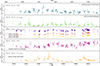 |
Fig. 1. Multi-wavelength light curves of Mrk 421 UV, Mrk 421 X-ray, Mrk 501 optical, Mrk 501 UV, and Mrk 501 X-ray. The legend shows the Swift telescope and filter used to collect the data, as well as the number of observations in each band. Each data point represents one observation. We present the full dynamic range of the data, in linear scaling, and observe higher variability at higher frequencies. |
In both sources, strong correlations within the optical bands, and strong correlations between the optical and UV bands, are observed. A strong correlation is said to be r ≥ 0.8, with r being the Pearson correlation coefficient. This is illustrated in Fig. A.1, and is expected because of the broad emissivity of photons in this wavelength range. Conversely, no simultaneous correlations are present between the optical/UV bands and X-ray band, though this is only strictly true when considering the entire period as one. However, if the X-ray data are divided by their spectral index, α, this is no longer true; see Fig. A.1. In theory we divide at α = 2, and spectra with α < 2 are called hard whereas spectra with α > 2 are called soft. In practice we divide the populations into  and
and  for each source (where
  is the mean spectral index), in order to create a safe boundary between them, accounting for errors. For Mrk 421 the upper and lower boundary values are 2.4 and 2.0, respectively, and for Mrk 501 they are 2.2 and 1.8, respectively. In both cases, hard X-rays versus UV and soft X-rays versus UV, we see an increase in correlation for each source, albeit on a low level. Interestingly, the magnitude of the increase in correlation is different between the sources. Specifically, in Mrk 421 the UV are more correlated with the hard X-rays than with the soft X-rays, whereas in Mrk 501 the UV are more correlated with the soft X-rays than with the hard X-rays. In general we may expect to see increased correlation between bands during flaring states, that is, hard X-ray spectral states, which is mildly observed in Mrk 421 but not in Mrk 501 (for the latter see, e.g., Fig. 2 in Abe et al. 2024), hinting at underlying differences in flare evolutions between the two sources. Notably, this is not visible when considering the whole dataset. Because the correlations are far below the r ≥ 0.8 level, and because dividing the X-rays greatly reduces the number of data points in each case (because of the ‘boundary’ between sub-populations), we do not make the index-based distinction again. Irrespective of the correlation value, the UV flux always covers the same range no matter the X-ray flux value or hardness state.
It is important to state that in these correlation plots in Fig. A.1, simultaneous observations are those taken within 0.1 days of each other. An in-depth discussion on the implications of correlations at varying time lags is provided in Sect. 3.6.
3.2. Fractional variability
The fractional variability, Fvar (Vaughan et al. 2003; Schleicher et al. 2019), of each band for both blazars is given in Table 1. It was calculated using
 (5)
(5)
Fractional variability in each filter of Mrk 421 and Mrk 501.
where S2 is the variance,  is the mean squared error, and
  is the mean flux. Its error is given by
 (6)
(6)
where N is the number of data points in the light curve. In both sources the fractional variability shows a clear dependence on energy (within the first SED peak), as is commonly seen in blazar observations (e.g., Sinha et al. 2016; Tantry et al. 2024; Abe et al. 2025). The X-rays have higher variability in contrast to the optical/UV photons. This statement is observed as presented in Table 1, and remains true if we correct for the worst case contribution of the host galaxy (not presented). This could be because X-rays are produced by more energetic electrons, which have the shorter cooling time, whereas optical/UV photons come from the lower-energy electron population, which takes longer to cool, and are hence less variable (Tantry et al. 2024; Abe et al. 2025).
Because of the strong correlations within the optical and with the UV data in Fig. 1, the similar fractional variability values, and the number of data points available in each band, all further analyses are carried out using only the UV and X-ray data. Of the > 1000 data points in each light curve, only a limited number of nights contain two observations, and the rest contain only one. Both sources are known to exhibit variability timescales as short as minutes in the X-ray regime (Zhang et al. 1999; Tramacere et al. 2009; Kapanadze et al. 2017a,b, 2018a,b); however, no short-term variability in the UV (Sambruna et al. 2000; Zeng et al. 2019; Chatterjee et al. 2021). For these reasons, we focus on only long-term variability in this paper.
3.3. Flux distributions
The flux distribution functions of the UV and X-ray flux of Mrk 421 and Mrk 501 are shown in the left (green) and right (purple) panels of Fig. 2, respectively. To each flux distribution, we fit a lognormal distribution, which is defined as
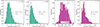 |
Fig. 2. Flux distributions for, from left to right, Mrk 421 UV, Mrk 421 X-ray, Mrk 501 UV, and Mrk 501 X-ray. The skewness parameter, γ, a metric of lognormality, is shown in the legend and increases with photon energy. |
 (7)
(7)
where m (units of ln(flux)) and s are the mean location and the shape parameters of the distribution, respectively. The skewness parameter, γ, of a lognormal distribution is written as
 (8)
(8)
and is presented for each fitted distribution in the figure legends. We see a positive trend of skewness with the frequency band; that is, the lognormality observed is energy-dependent.
The lognormal distribution of flux has been commonly observed at high energies in blazars: first in the X-ray band for BL Lacertae (Giebels & Degrange 2009), then in the γ ray band for many sources (e.g., H.E.S.S. Collaboration 2010, 2017; Bhatta & Dhital 2020). For Mrk 421, lognormality has also been observed in the lower-energy radio and optical bands (Sinha et al. 2016), and in the optical and UV bands (Kapanadze et al. 2024). We have found a trend of weaker lognormality toward longer wavelengths, which is in line with the results of Ciaramella et al. (2004), H.E.S.S. Collaboration (2017), and Kapanadze et al. (2023). This is expected in the case of random fluctuations in the particle acceleration rate caused by small temporal fluctuations in the accretion disc (Sinha et al. 2018).
A characteristic of the lognormal process is that fluctuations in the flux are, on average, proportional to the flux itself (Aitchinson & Brown 1963); that is to say, the root-mean-square–flux relation is linear (Uttley & McHardy 2001). In blazars, these processes are often attributed to stochastic multiplicative processes (Uttley et al. 2005), and linked to the underlying accretion process of the disc on the jet (Uttley & McHardy 2001; Giebels & Degrange 2009). If damping is negligible, density fluctuations and instabilities in the disc, arising on local viscous timescales, can propagate inwards and couple together so as to produce a multiplicative behaviour in the accretion rate (see Rieger 2019 and references therein). If this effect were efficiently transmitted into the jet, the emission could be modified accordingly (H.E.S.S. Collaboration 2017). Other possible multiplicative processes occurring in blazars are cascade-like events such as synchrotron radiation from the proton-induced hadronic cascades (H.E.S.S. Collaboration 2017; Rieger 2019), or the jets-in-jets scenario (Biteau & Giebels 2012), in which magnetic dissipation triggers the emission of relativistic smaller jets of plasma within the bulk of the jet. It is critically important to note that this latter model reconciles the flux properties and rapid variations present in blazars at high (γ ray) energies, but research has yet to establish whether it can also explain the lognormal distributions observed at lower (optical, UV, X-ray) energies (Li et al. 2017).
Whilst all of these multiplicative mechanisms are possible, Biteau & Giebels (2012) and Scargle (2020) showed that a lognormal distribution can in fact come also from a series of additive processes, meaning that shot noise, or the superposition of many minijets, could also explain the observed flux distributions. Bhatta & Dhital (2020) suggest a scenario in which both additive and multiplicative processes operate at varying degrees along the extended jet. Sinha et al. (2018) and references therein also point out that the rapid variability seen in X-ray strongly favour mechanisms within the jet, rather than in the accretion disc. The fact that we observe lognormal flux distributions of quite different skewnesses in different energy bands is an indication that these photons are not coming from the same emission zones; hence, a multi-zone model is required to fully explain the blazar’s emission processes (Kapanadze et al. 2020, 2023, 2024).
3.4. Photon indices
The values of the α and β parameters used in the LP fitting of the X-ray data, as described in Eq. (4), are plotted in the top (green) and bottom (purple) panels of Fig. 3 for Mrk 421 and Mrk 501, respectively. Alpha values are comparable to the photon index in a power law fit, Γ in Eq. (3), and these terms are hereafter used interchangeably. The X-ray photon index of Mrk 421 varies from 1.47 to 2.98, and that of Mrk 501 from 1.49 to 2.80. As is illustrated by the colour bar, both sources fluctuate over time between hard and soft states: a hard photon spectrum has Γ < 2, and a soft one has Γ > 2. Moving from soft to hard spectra indicates that the synchrotron peak position shifts to higher energies and that the HBLs become ‘extreme’ HBLs (Ahnen et al. 2018; Abeysekara et al. 2020). Malkov & Drury (2001) showed that multiple shocks are required in order to produce photon indices as hard as ∼1.5.
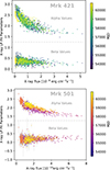 |
Fig. 3. X-ray log parabola fit parameters, α and β, as a function of flux. Mrk 421 (top) and Mrk 501 (bottom) follow the harder-when-brighter trend, with no trend in curvature. |
The β parameter, that is, curvature, shows no trend with flux but does show significant variations between observations. It has an average value of 0.352 ± 0.035 for Mrk 421, and 0.176 ± 0.080 for Mrk 501, showing that the spectra of the former are consistently more curved than the latter. In Mrk 501 the β parameter falls below 0 for some data points, meaning that the spectra change shape from concave to convex, which could also be caused by a shift in synchrotron peak position. There is no correlation observed between α and β in either source.
For both sources, the anti-correlation of alpha and flux is indicative of the harder-when-brighter trend seen in many blazars, including Mrk 421 (Kapanadze et al. 2020, 2024; Alfaro et al. 2025) and Mrk 501 (Kapanadze et al. 2023; Abe et al. 2024; Tantry et al. 2024; Alfaro et al. 2025). This trend, that is, the hardening of the spectrum with increasing flux, can be caused by electrons that are rapidly accelerated compared to the rate at which they cool. The phases of increasing flux are when the spectra harden, and those of decreasing flux are when they soften. This flaring behaviour can be reproduced by the shock-in-jet model with escape and synchrotron losses (Kirk et al. 1998): a shock propagates through the plasma and increases the plasma’s local density, which quickly involves more particles in the acceleration process (Sokolov et al. 2004).
3.5. Periodicity search
Studies of periodicities, or of QPOs, which are more likely to be present, can be used to infer the physical dimensions, masses, and geometrical structures of emission zones (Ghisellini et al. 2010). In order to thoroughly investigate any potential QPOs present in the UV and X-ray light curves of Mrk 421 and Mrk 501, we employed three well-known techniques: the structure function (SF), the Lomb-Scargle periodogram (LSP), and the discrete auto-correlation function (DACF).
The first-order structure function (Rutman 1978; Simonetti et al. 1985) is defined as
![Mathematical equation: $$ \begin{aligned} \mathrm{SF}(\tau ) = \frac{1}{N}\sum _{i = 1}^N \left[X(t_i) - X(t_i + \tau )\right]^2, \end{aligned} $$](/articles/aa/full_html/2026/02/aa57635-25/aa57635-25-eq17.gif) (9)
(9)
where X(ti) is the flux measured at time ti, the total number of pairs of measurements is N, and X(ti) and X(ti + τ) are pairs of flux measurements separated by a time lag, τ. The SF has the advantage of being less affected by windowing effects, often seen in blazar light curves due to the large gaps between observation periods, compared to direct Fourier methods (H.E.S.S. Collaboration 2010). Interpretation of the SF is an intricate deed, and commonly the break seen at longer time lag values, for example around 2000 days for Mrk 501 in Fig. 4, is wrongly credited as the characteristic timescale of the source (the QPO). Emmanoulopoulos et al. (2010) show that it in fact represents the characteristic timescale of the light curve: it is the maximum probeable timescale given the length of the observations. The SFs can therefore be used to provide upper limits to timescale investigations such as our own. Since each of the light curves is slightly longer than 7000 days, timescales of longer than 1400 days are probed with fewer than five independent samples, and hence cannot be explored with reliable statistical significance. We thus set an upper limit for probing timescales with the LSP and DACF at ∼1400 days. The SFs for Mrk 421 and Mrk 501 both using UV and X-ray data are displayed in Fig. 4. All SF decay in a power law fashion towards short timescales. The break usually seen at lower time lag values, which represents the timescale in which average variability amplitudes are comparable to the average measurement errors, is not observed in our work due to the cadence of the light curves (see Sect. 3.2). Both SFs of Mrk 501 rise in a power law fashion up to breaks beyond the longest timescales that can be probed (about 1400 days). The X-ray SF of Mrk 421 breaks on timescales of 30−100 days, with a significant change in the power law slope displayed over more than one order of magnitude towards shorter and longer timescales. A similar break is indicated in the SF of UV variations of Mrk 421, but is only marginally significant. Beyond 3000 days both SFs of Mrk 421 display further deviations from a power-law SF, but at these timescales they no longer provide statistically meaningful information.
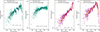 |
Fig. 4. Structure functions for Mrk 421 UV (far left), Mrk 421 X-ray (centre left), Mrk 501 UV (centre right), and Mrk 501 X-ray (far right). After 2000 days these are badly affected by systematics, so peaks right of this value should not be trusted. Only Mrk 421 X-ray appears to reach saturation. |
Various peaks and troughs are seen in the SFs in Fig. 4, perhaps most clearly in Mrk 421 UV, but in all cases these are found at multiples of half a year. They should therefore not be interpreted as physical timescales associated with the blazars.
The LSP (Lomb 1976; Scargle 1982) is defined as
![Mathematical equation: $$ \begin{aligned} \begin{aligned} P(f) =&\frac{A^2}{2}\left(\sum _n g_n\cos (2\pi f[t_n-\tau ]\right)^2\\&+ \frac{B^2}{2}\left(\sum _n g_n\sin (2\pi f[t_n-\tau ]\right)^2, \end{aligned} \end{aligned} $$](/articles/aa/full_html/2026/02/aa57635-25/aa57635-25-eq18.gif) (10)
(10)
where A, B, and τ are arbitrary functions of the frequency, f, and observing times, {ti} (VanderPlas 2018). Incorporating Fourier analysis, the least-squares method, and Bayesian probability theory, the LSP’s strength lies in its ability to examine QPOs in unevenly sampled time series. The standard LSP does not account for measurement errors, and assumes that the fitted sine function has the same mean as the data. Hence, we used the generalised LSP (Zechmeister & Kürster 2009) to avoid these shortcomings. In order to assess the validity of peaks in the LSP, we employed the false alarm probability (FAP) method (Baluev 2008) and the Monte Carlo method. For the latter, we generated 10 000 synthetic light curves with the same power spectral density, probability density function, and sampling as the observed light curves, following the Emmanoulopoulos et al. (2013) algorithm implemented in the gammapy_SyLC package1, and necessitated a significance of ≥3σ (Vaughan 2005). Matching the cadence of the observations in the synthetic light curves intrinsically accounts for any aliases that would occur due to windowing.
The LSPs for Mrk 421 UV and X-ray, and Mrk 501 UV and X-ray, are displayed in Fig. 5. There are no potential QPOs detected in the UV light curves of Mrk 421 or Mrk 501. The X-ray LSP of Mrk 421 shows 11 peaks between 37 and 125 days, but after careful inspection of the peaks in the same time frame for the synthetic light curves we conclude that these QPOs should not be interpreted as genuine. This is because many peaks appear in the same range of time lag values in almost all of the synthetic LSPs, but are not reflected in the grey significance bands due to slight shifts in the exact time at which each peak appears. There is a potential QPO detected above the required 3σ significance level and the 5σ FAP in the X-ray LSP of Mrk 501 at  days. The uncertainties here were estimated by fitting a skewed Gaussian and calculating its two half width at half maximum values. These results will be discussed further in this section, after the DACF results.
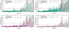 |
Fig. 5. Lomb-Scargle periodograms for Mrk 421 UV (top left), Mrk 421 X-ray (top right), Mrk 501 UV (bottom left), and Mrk 501 X-ray (bottom right). Only the latter contains a peak above the 3σ significance level, which falls at around 400 days. |
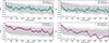 |
Fig. 6. Discrete auto-correlation functions for Mrk 421 UV (top left), Mrk 421 X-ray (top right), Mrk 501 UV (bottom left), and Mrk 501 X-ray (bottom right). Again only the latter contains any points above the 3σ significance level, at around 1400 days. |
The third approach we used to investigate possible QPOs was the DACF, which is a special case of the discrete correlation function (DCF, Edelson & Krolik 1988) where the same time series is correlated with itself. The DCF is defined as
 (11)
(11)
where a and b are the values (in our case, fluxes) of the time series, with mean values  and
and  , and standard deviations σa and σb, respectively. N is the number of pairs, i, j, in the time interval, τ. In the DACF, a = b, and we are able to investigate timescales intrinsic to the light curve. We generated synthetic light curves following the same structure as was outlined for the LSPs to create significance contours for the DACFs. Due to the colour noise nature of blazars (Press 1978; Lawrence et al. 1987), we expect the DACF value to slowly decrease as time lag increases, representing the inherent auto-correlation present in these sources. Points of interest are therefore: the time lag value at which this decreasing trend breaks, how clearly it breaks, and any distinct peaks (or troughs) exceeding the 3σ significance bands.
The DACFs for Mrk 421 UV and X-ray, and Mrk 501 UV and X-ray, are displayed in Fig. 6. In Mrk 421 UV and X-ray, breaks appear at ∼84 days and ∼42 days, respectively, where the latter of these results is a harmonic of the former, indicating a possibly genuine QPO. After roughly 200 days, both Mrk 421 DACFs begin to fluctuate around zero, indicating no auto-correlation after this time lag. The DACFs of Mrk 501 UV and X-ray show a variety of features between 25 and 280 days. Included in both is a peak at roughly 200 days, but this is not > 3σ significant. No significant features appears to be present at ∼400 days in the Mrk 501 UV or X-ray DACFs, where the potential QPO lay in the corresponding LSP, but it is worth mentioning that the 200 day peak corresponds to a harmonic of the 400 day LSP peak. Also interesting to note is the > 3σ trough in the Mrk 501 DACF at ∼1400 days: for a time series with period T, a negative auto-correlation value occurs when the time lag examined is out of phase with the dominant peak in the light curve; that is, (n + 1/2)T. If T = 400 days from the LSP, then the trough falls exactly at n = 3. At roughly n = 2, or a time lag of 1000 days, is another trough that falls just below 3σ significance.
At n = 1 (600 days) the strongest aliasing feature would be expected, but is not observed. In the Mrk 501 UV LSP in Fig. 5 we see a peak at ∼400 days, and peaks corresponding to harmonics at ∼200 and ∼600 days that are > 2σ significant.
There is a lack of consistency between the LSPs and DACFs, as well as within the DACFs themselves; for example, troughs appear at n = 2 and n = 3, but not at n = 1, and no significant peaks (nT) appear at any value of n. These inconsistencies do not strengthen the indication of any QPO results. Mainly, they highlight the necessity for more densely sampled light curves in blazar analyses.
To the best of our knowledge, currently no QPOs have been reported for Mrk 421 in the UV or optical bands, despite efforts by, for example, Carnerero et al. (2017), Sandrinelli et al. (2017), Tarnopolski et al. (2020), Kapanadze et al. (2020, 2024), Otero-Santos et al. (2023), and Abe et al. (2025), all of whom also found no QPOs in any other band. The latter statement is contradictory to the work of, for example, Li et al. (2016), Bhatta & Dhital (2020), and Ren et al. (2023), who found QPOs ranging from 278−310 days at radio, X-ray, and/or gamma-ray energies.
Over the years, QPOs in Mrk 501 have been reported at varying timescales: ∼23 days, or harmonics thereof, by Hayashida et al. (1998), Protheroe et al. (1998), Kranich et al. (1999), Nishikawa et al. (1999), and Roedig et al. (2009) in the X-ray and/or gamma-rays; and 330 and 333 days in the gamma and the optical by Bhatta (2019, 2021), respectively. Possible mechanisms responsible for the ∼23 day QPO has been investigated thoroughly (Rieger & Mannheim 2000; Rieger 2005; Yu-Hai & Jiang-He 2005; Fan et al. 2008). Both Devanand et al. (2022) and Kapanadze et al. (2023) found no QPOs at UV, X-ray, and/or gamma-ray energies. We believe this is the first time a possible QPO of ∼400 days has been reported for Mrk 501. Because 400 days is a year-like timescale, we have taken care to check that this peak is not just a consequence of windowing and that it does not appear in the Mrk 501 UV LSP if only the data with matching MJD values (within 0.1 days) to the Mrk 501 X-ray light curve are used.
In its host frame, the reported QPO in Mrk 501 corresponds to  days, using P′=Pobs/(1 + z). We offer three possible explanations for this observation. The first is a supermassive binary black hole (SMBBH) system in which the less massive black hole emits nonthermal radiation via its relativistic jet (Valtonen et al. 2011). The jet exhibits orbital motion around the system’s centre of mass, which means the Doppler factor for the emission region is a periodic function of time (Rieger & Mannheim 2000). This model can also produce complex QPOs due to mergers and other such interactions (Valtonen et al. 2008). Whilst SMBBHs are possible, the number of year-like physical periods (P′) detected in blazars, for example in this work for Mrk 501, are unlikely to all be caused by such systems due to gravitational constraints (Rieger 2019).
The second explanation stems from the helical motion of a component inside a jet, which itself is rotating, where differential Doppler boosting explains periodic lighthouse effects (Camenzind & Krockenberger 1992). This model is closely linked to the model of Schramm et al. (1993) and has a dynamical timescale of days to years. However, in such models long-timescale QPOs do not complete many oscillations; hence, their signal is drowned out. We therefore cannot credit this mechanism with the production of the 390 day (host frame) QPO that we observe.
The third scenario is concerned with instabilities intrinsic to the accretion disc McHardy et al. (2006), such as bright hot-spots orbiting on the disc (Bhatta 2018), Lense-Thirring precession (Stella & Vietri 1998), and jet precession due to a warped accretion discs (Liska et al. 2018). Of these accretion disc scenarios, the first two can be on the same timescales as the QPOs found in this work, but the latter cannot, expecting ∼103 years (Liska et al. 2018). Chatterjee et al. (2018) point out that if it is the accretion disc which regulates the jet emission, or creates the shocks that move through the jet, then QPOs found in any energy band should be the same for the same source. This means that all reported QPOs should be close in value. If we believe that our QPO is a result of the imprinting of the disc onto the jet, this is also supported by the lognormality observed in the flux distributions in Sect. 3.3, which can be explained in the same way (Uttley & McHardy 2001). Similarly, Arbet-Engels et al. (2021b) found a characteristic time between tera-electronvolt flares in Mrk 501 of 5−25 days, which is comparable to the timescale associated with flares triggered by Lense-Thirring precession of the accretion disc. Together these results provide evidence for a disc-jet connection in Mrk 501, despite the lack of directly observed disc features.
The lack of detections of QPOs in Mrk 421 UV and X-ray and Mrk 501 UV are still valuable in that they provide lower limits for any QPOs that may exist in these objects at these energies. That is, both sources may have genuine QPOs that are simply longer than timescales we are able to reasonably probe: > 1400 days. Of course, we have also limited our search to QPOs longer than 3−5 days due to sampling constraints. Thus, an upper limit to QPO period is also imposed. For a full discussion of factors limiting QPO detections, see Vaughan & Uttley (2005).
3.6. Cross-correlations
As was mentioned in Sect. 3.1, simultaneous correlations between optical and UV bands, such as those seen in Fig. A.1, are expected due to the broad-band emissivity of photons in that energy range. This has frequently been confirmed to be true; for example, by Kapanadze et al. (2016, 2017a,b, 2018a,b, 2020, 2023, 2024) and Abe et al. (2025). All of these researchers also found no or only weak long-term simultaneous correlations between the optical/UV and X-ray bands, as we have in Sect. 3.1.
Moreover, we used the discrete cross-correlation function (DCCF), defined in Eq. (11) with a ≠ b, to investigate if the optical/UV bands lead or lag behind the X-ray band. The length of our light curves allows us to probe longer than ever lag ranges. We limit this study to lags between −1400 and 1400 for the same reasons that are given in Sect. 3.5. The UV versus X-ray DCCFs for Mrk 421 and Mrk 501 are shown in the top and bottom panel of Fig. 7, respectively, with the grey significance bands generated in exactly the same way as with the DACFs in Sect. 3.5. Neither source shows any significant correlation at any given lead or lag, by either band. We cannot, however, exclude cross-correlations on timescales of a day or less, for the same sampling reasons as are explained in Sects. 3.2 and 3.5.
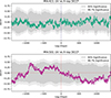 |
Fig. 7. UV vs X-ray discrete cross-correlation functions for Mrk 421 (top) and Mrk 501 (bottom). |
When focussing on shorter defined periods of specific flares, Kapanadze et al. (2016, 2017a, 2018b, 2020, 2023, 2024) found weak but statistically significant simultaneous positive correlations between the X-ray and optical/UV bands. In fact, in Kapanadze et al. (2018b, 2020) these correlations are also negative in some periods. Using the entire period of our light curves we confirm that, whilst during certain periods a quasi-simultaneous X-ray – optical/UV correlation may be present, overall it is not. This gives further evidence for the multi-zone model, and even suggests that the number of zones is not constant but changing; hence, why sometimes correlations do appear, but inconsistently.
Given that both sources are classified as HBLs, the X-ray emission falls within the lower energy peak in the SED (Abdo et al. 2010), which implies an optical/UV–X-ray correlation under the one-zone model. Recent work on X-ray polarisation data by Liodakis et al. (2022) suggests a shock front in the jet as the source of particle acceleration, which also insinuates optical/UV–X-ray correlation. Conversely, the lack of correlation observed in this work, and in work by Kapanadze et al. (2020, 2023, 2024), Abe et al. (2024, 2025), suggests a multi-zone model. Observations and modelling of an intriguing case of a blazar showing evidence for the multi-zone model can be found in H.E.S.S. Collaboration (2023).
4. Conclusions
The HBLs Mrk 421 and Mrk 501 have been observed for 20 years, from 2005 to 2025, with the Swift-UVOT and Swift-XRT telescopes, providing us with rich MWL datasets and valuable insights into the nature of blazars. We investigated long-term trends and summarise our key findings as follows:
-
The Swift X-ray spectra studied in this work are statistically better fit with a log parabola model than a single power law.
-
Sub-populations of the X-ray data, defined by hard and soft spectral states, show an increase in correlation with the UV data, in contrast to that of the whole population.
-
Fractional variability is dependent on energy for both sources. This could be due to the cooling times of the electron populations that produce the respective photons (Tantry et al. 2024; Abe et al. 2025).
-
The fluxes follow a lognormal distribution, but much more pronouncedly in the X-rays than in the optical/UV, for both blazars. Lognormal distributions may be created by additive or multiplicative processes (or a combination of the two) (Uttley & McHardy 2001; Sinha et al. 2018; Scargle 2020). The energy dependence of the distributions can be explained by fluctuations in the particle acceleration rate, which begin as fluctuations in the accretion disc (Sinha et al. 2018). The differing distribution shapes are supportive of a multi-zone model.
-
X-ray photon indices vary with flux following a general harder-when-brighter trend, signifying that the rate at which electrons are accelerated is much faster than the rate at which they cool. This flaring activity indicates a rapid variability in the number of electrons producing X-ray photons.
-
The X-ray photon indices also shift from hard to soft and back again many times over the 20 years of observations, reflecting the phases of flux increases (spectral hardening), and flux decreases (spectral softening). This means that shifts in the position of the synchrotron SED peak have occurred.
-
An in-depth time series analysis has revealed a potential QPO of ∼390 days (host frame) for Mrk 501 in the X-ray. On this timescale, QPOs can be explained by accretion disc instabilities such as hot spots and Lense-Thirring precession (Stella & Vietri 1998; Bhatta 2018). The lack of detections of QPOs in Mrk 421 UV and X-ray, and Mrk 501 UV, imply QPO limits of < 3 days or > 1400 days and < 4 days or > 1400 days, respectively.
-
Strong optical–UV correlations were observed at zero time lag, but none were for optical/UV–X-ray correlations in any lag between −1400 and 1400 days. This contradicts the implications of a one-zone model, in which all wavelengths within the lower SED peak should be well correlated, again giving evidence for a multi-zone emission model.
Overall, this work gives a comprehensive analysis of the temporal characteristics of Mrk 421 and Mrk 501 in the UV and X-ray bands as recorded by Swift. These results strongly favour a multi-zone model to explain the emissions of Mrk 421 and Mrk 501 over the last 20 years.
Acknowledgments
We thank the anonymous referee for their constructive feedback, which helped to improve the manuscript. We also wish to thank Frank Rieger, Sarah Wagner, and Daniela Dorner for interesting and very helpful discussions at the DFG RU 5195 Annual Assembly 2025 and elsewhere. We gratefully acknowledge funding by the Deutsche Forschungsgemeinschaft (DFG, German Research Foundation), within the research unit 5195 “Relativistic Jets in Active Galaxies” – project number 443220636. The project on which this report is based was partially funded by the Bundesministerium für Bildung und Forschung (BMBF, Ministry of Education and Research). Responsibility for the content of this publication lies with the author. The project is co-financed by the Polish National Agency for Academic Exchange. The authors gratefully acknowledge the Polish high-performance computing infrastructure PLGrid (HPC Center: ACK Cyfronet AGH) for providing computer facilities and support within computational grant no. PLG/2024/017925. This work is funded in parts by the Deutsche Forschungsgemeinschaft (DFG, German Research Foundation) – project number 460248186 (PUNCH4NFDI).
References
- Abdo, A. A., Ackermann, M., Agudo, I., et al. 2010, ApJ, 716, 30 [NASA ADS] [CrossRef] [Google Scholar]
- Abe, S., Abhir, J., Acciari, V. A., et al. 2024, A&A, 685, A117 [NASA ADS] [CrossRef] [EDP Sciences] [Google Scholar]
- Abe, K., Abe, S., Abhir, J., et al. 2025, A&A, 694, A195 [NASA ADS] [CrossRef] [EDP Sciences] [Google Scholar]
- Abeysekara, A. U., Benbow, W., Bird, R., et al. 2020, ApJ, 890, 97 [NASA ADS] [CrossRef] [Google Scholar]
- Ahnen, M. L., Ansoldi, S., Antonelli, L. A., et al. 2016, A&A, 593, A91 [NASA ADS] [CrossRef] [EDP Sciences] [Google Scholar]
- Ahnen, M. L., Ansoldi, S., Antonelli, L. A., et al. 2018, A&A, 620, A181 [NASA ADS] [CrossRef] [EDP Sciences] [Google Scholar]
- Aitchinson, J., & Brown, J. A. C. 1963, The Lognormal Distribution (Cambridge: Cambridge University Press) [Google Scholar]
- Alfaro, R., Alvarez, C., Andrés, A., et al. 2025, ApJ, 980, 88 [Google Scholar]
- Arbet-Engels, A., Baack, D., Balbo, M., et al. 2021a, A&A, 647, A88 [NASA ADS] [CrossRef] [EDP Sciences] [Google Scholar]
- Arbet-Engels, A., Baack, D., Balbo, M., et al. 2021b, A&A, 655, A93 [NASA ADS] [CrossRef] [EDP Sciences] [Google Scholar]
- Arnaud, K. A. 1996, ASP Conf. Ser., 101, 17 [Google Scholar]
- Baluev, R. V. 2008, MNRAS, 385, 1279 [Google Scholar]
- Bevington, P. R., & Robinson, D. K. 2003, Data Reduction and Error Analysis for the Physical Sciences (New York: McGraw-Hill) [Google Scholar]
- Bhatta, G. 2018, Galaxies, 6, 136 [Google Scholar]
- Bhatta, G. 2019, MNRAS, 487, 3990 [NASA ADS] [CrossRef] [Google Scholar]
- Bhatta, G. 2021, ApJ, 923, 7 [CrossRef] [Google Scholar]
- Bhatta, G., & Dhital, N. 2020, ApJ, 891, 120 [NASA ADS] [CrossRef] [Google Scholar]
- Biteau, J., & Giebels, B. 2012, A&A, 548, A123 [NASA ADS] [CrossRef] [EDP Sciences] [Google Scholar]
- Blandford, R. D., & Rees, M. J. 1974, MNRAS, 169, 395 [NASA ADS] [CrossRef] [Google Scholar]
- Błażejowski, M., Sikora, M., Moderski, R., & Madejski, G. M. 2000, ApJ, 545, 107 [Google Scholar]
- Błażejowski, M., Blaylock, G., Bond, I. H., et al. 2005, ApJ, 630, 130 [Google Scholar]
- Böttcher, M. 2007, Ap&SS, 307, 69 [CrossRef] [Google Scholar]
- Burrows, D. N., Hill, J. E., Nousek, J. A., et al. 2005, Space Sci. Rev., 120, 165 [Google Scholar]
- Camenzind, M., & Krockenberger, M. 1992, A&A, 255, 59 [NASA ADS] [Google Scholar]
- Carnerero, M. I., Raiteri, C. M., Villata, M., et al. 2017, MNRAS, 472, 3789 [NASA ADS] [CrossRef] [Google Scholar]
- Catanese, M., Bradbury, S. M., Breslin, A. C., et al. 1997, ApJ, 487, L143 [Google Scholar]
- Cerruti, M. 2020, Galaxies, 8, 72 [NASA ADS] [CrossRef] [Google Scholar]
- Chatterjee, R., Roychowdhury, A., Chandra, S., & Sinha, A. 2018, ApJ, 859, L21 [NASA ADS] [CrossRef] [Google Scholar]
- Chatterjee, R., Das, S., Khasnovis, A., et al. 2021, JApA, 42, 80 [NASA ADS] [Google Scholar]
- Ciaramella, A., Bongardo, C., Aller, H. D., et al. 2004, A&A, 419, 485 [NASA ADS] [CrossRef] [EDP Sciences] [Google Scholar]
- Cui, W. 2004, ApJ, 605, 662 [Google Scholar]
- Dermer, C. D., Schlickeiser, R., & Mastichiadis, A. 1992, A&A, 256, L27 [NASA ADS] [Google Scholar]
- Devanand, P. U., Gupta, A. C., Jithesh, V., & Wiita, P. J. 2022, ApJ, 939, 80 [NASA ADS] [CrossRef] [Google Scholar]
- Edelson, R. A., & Krolik, J. H. 1988, ApJ, 333, 646 [Google Scholar]
- Emmanoulopoulos, D., McHardy, I. M., & Uttley, P. 2010, MNRAS, 404, 931 [NASA ADS] [CrossRef] [Google Scholar]
- Emmanoulopoulos, D., McHardy, I. M., & Papadakis, I. E. 2013, MNRAS, 433, 907 [NASA ADS] [CrossRef] [Google Scholar]
- Fan, J., Rieger, F., Hua, T., et al. 2008, Astropart. Phys., 28, 508 [Google Scholar]
- Ghisellini, G., Tavecchio, F., Foschini, L., et al. 2010, MNRAS, 402, 497 [Google Scholar]
- Giebels, B., & Degrange, B. 2009, A&A, 503, 797 [NASA ADS] [CrossRef] [EDP Sciences] [Google Scholar]
- Giommi, P., Blustin, A. J., Capalbi, M., et al. 2006, A&A, 456, 911 [NASA ADS] [CrossRef] [EDP Sciences] [Google Scholar]
- Graff, P. B., Georganopoulos, M., Perlman, E. S., & Kazanas, D. 2008, ApJ, 689, 68 [CrossRef] [Google Scholar]
- H.E.S.S. Collaboration (Abramowski, A., et al.) 2010, A&A, 520, A83 [NASA ADS] [CrossRef] [EDP Sciences] [Google Scholar]
- H.E.S.S. Collaboration (Abramowski, A., et al.) 2014, A&A, 571, A39 [NASA ADS] [CrossRef] [EDP Sciences] [Google Scholar]
- H.E.S.S. Collaboration (Abdalla, H., et al.) 2017, A&A, 598, A39 [NASA ADS] [CrossRef] [EDP Sciences] [Google Scholar]
- H.E.S.S. Collaboration (Aharonian, F., et al.) 2023, ApJ, 952, L38 [NASA ADS] [Google Scholar]
- Hayashida, N., Hirasawa, H., Ishikawa, F., et al. 1998, ApJ, 504, L71 [Google Scholar]
- HI4PI Collaboration (Ben Bekhti, N., et al.) 2016, A&A, 594, A116 [NASA ADS] [CrossRef] [EDP Sciences] [Google Scholar]
- Kapanadze, B., Dorner, D., Vercellone, S., et al. 2016, ApJ, 831, 102 [NASA ADS] [CrossRef] [Google Scholar]
- Kapanadze, B., Dorner, D., Romano, P., et al. 2017a, ApJ, 848, 103 [Google Scholar]
- Kapanadze, B., Dorner, D., Romano, P., et al. 2017b, MNRAS, 469, 1655 [NASA ADS] [CrossRef] [Google Scholar]
- Kapanadze, B., Vercellone, S., Romano, P., et al. 2018a, ApJ, 854, 66 [Google Scholar]
- Kapanadze, B., Vercellone, S., Romano, P., et al. 2018b, ApJ, 858, 68 [NASA ADS] [CrossRef] [Google Scholar]
- Kapanadze, B., Gurchumelia, A., Dorner, D., et al. 2020, ApJS, 247, 27 [NASA ADS] [CrossRef] [Google Scholar]
- Kapanadze, B., Gurchumelia, A., & Aller, M. 2023, ApJS, 268, 20 [Google Scholar]
- Kapanadze, B., Gurchumelia, A., & Aller, M. 2024, ApJS, 275, 23 [Google Scholar]
- Kapanadze, B., Gurchumelia, A., & Aller, M. 2025, Ap&SS, 370, 17 [Google Scholar]
- Kirk, J. G., Rieger, F. M., & Mastichiadis, A. 1998, A&A, 333, 452 [NASA ADS] [Google Scholar]
- Kranich, D., de Jager, O., Kestel, M., et al. 1999, 26th International Cosmic Ray Conference, 3, 358 [Google Scholar]
- Lawrence, A., Watson, M. G., Pounds, K. A., & Elvis, M. 1987, Nature, 325, 694 [Google Scholar]
- Li, H. Z., Jiang, Y. G., Guo, D. F., Chen, X., & Yi, T. F. 2016, PASP, 128, 074101 [Google Scholar]
- Li, Y. T., Hu, S. M., Jiang, Y. G., et al. 2017, PASP, 129, 014101 [Google Scholar]
- Liodakis, I., Marscher, A. P., Agudo, I., et al. 2022, Nature, 611, 677 [CrossRef] [Google Scholar]
- Liska, M., Hesp, C., Tchekhovskoy, A., et al. 2018, MNRAS, 474, L81 [Google Scholar]
- Lomb, N. R. 1976, Ap&SS, 39, 447 [Google Scholar]
- Malkov, M. A., & Drury, L. O. 2001, Rep. Progr. Phys., 64, 429 [Google Scholar]
- Mannheim, K. 1993, A&A, 269, 67 [NASA ADS] [Google Scholar]
- McHardy, I. M., Koerding, E., Knigge, C., Uttley, P., & Fender, R. P. 2006, Nature, 444, 730 [NASA ADS] [CrossRef] [Google Scholar]
- Nishikawa, D., Hayashi, S., Chamoto, N., et al. 1999, 26th International Cosmic Ray Conference, 3, 354 [Google Scholar]
- Otero-Santos, J., Peñil, P., Acosta-Pulido, J. A., et al. 2023, MNRAS, 518, 5788 [Google Scholar]
- Padovani, P., & Giommi, P. 1995, ApJ, 444, 567 [NASA ADS] [CrossRef] [Google Scholar]
- Pánis, R., Bhatta, G., Adhikari, T. P., et al. 2025, ApJ, 989, 106 [Google Scholar]
- Poole, T. S., Breeveld, A. A., Page, M. J., et al. 2008, MNRAS, 383, 627 [Google Scholar]
- Press, W. H. 1978, Comments Astrophys., 7, 103 [NASA ADS] [Google Scholar]
- Protheroe, R., Bhat, C., Fleury, P., et al. 1998, 25th International Cosmic Ray Conference, 8, 317 [Google Scholar]
- Punch, M., Akerlof, C., Cawley, M., et al. 1992, Nature, 358, 477 [NASA ADS] [CrossRef] [Google Scholar]
- Quinn, J., Akerlof, C. W., Biller, S., et al. 1996, ApJ, 456, L83 [NASA ADS] [Google Scholar]
- Ren, H. X., Cerruti, M., & Sahakyan, N. 2023, A&A, 672, A86 [NASA ADS] [CrossRef] [EDP Sciences] [Google Scholar]
- Rieger, F. M. 2005, Chin. J. Astron. Astrophys., 5, 305 [Google Scholar]
- Rieger, F. M. 2019, Galaxies, 7, 28 [Google Scholar]
- Rieger, F. M., & Mannheim, K. 2000, A&A, 359, 948 [NASA ADS] [Google Scholar]
- Roedig, C., Burkart, T., Elbracht, O., & Spanier, F. 2009, A&A, 501, 925 [Google Scholar]
- Roming, P. W. A., Kennedy, T. E., Mason, K. O., et al. 2005, Space Sci. Rev., 120, 95 [Google Scholar]
- Rutman, J. 1978, Proc. IEEE, 66, 1048 [NASA ADS] [CrossRef] [Google Scholar]
- Sambruna, R. M., Aharonian, F. A., Krawczynski, H., et al. 2000, ApJ, 538, 127 [Google Scholar]
- Sandrinelli, A., Covino, S., Treves, A., et al. 2017, A&A, 600, A132 [NASA ADS] [CrossRef] [EDP Sciences] [Google Scholar]
- Scargle, J. D. 1982, ApJ, 263, 835 [Google Scholar]
- Scargle, J. D. 2020, ApJ, 895, 90 [NASA ADS] [CrossRef] [Google Scholar]
- Schlafly, E. F., & Finkbeiner, D. P. 2011, ApJ, 737, 103 [Google Scholar]
- Schleicher, B., Arbet-Engels, A., Baack, D., et al. 2019, Galaxies, 7, 62 [NASA ADS] [CrossRef] [Google Scholar]
- Schramm, K.-J., Borgeest, U., Camenzind, M., et al. 1993, A&A, 278, 391 [NASA ADS] [Google Scholar]
- Sikora, M., Begelman, M. C., & Rees, M. J. 1994, ApJ, 421, 153 [Google Scholar]
- Simonetti, J. H., Cordes, J. M., & Heeschen, D. S. 1985, ApJ, 296, 46 [NASA ADS] [CrossRef] [Google Scholar]
- Sinha, A., Shukla, A., Saha, L., et al. 2016, A&A, 591, A83 [NASA ADS] [CrossRef] [EDP Sciences] [Google Scholar]
- Sinha, A., Khatoon, R., Misra, R., et al. 2018, MNRAS, 480, L116 [NASA ADS] [CrossRef] [Google Scholar]
- Sokolov, A., Marscher, A. P., & McHardy, I. M. 2004, ApJ, 613, 725 [NASA ADS] [CrossRef] [Google Scholar]
- Stella, L., & Vietri, M. 1998, ApJ, 492, L59 [NASA ADS] [CrossRef] [Google Scholar]
- Tantry, J., Shah, Z., Misra, R., Iqbal, N., & Akbar, S. 2024, J. High Energy Astrophys., 44, 393 [Google Scholar]
- Tarnopolski, M., Żywucka, N., Marchenko, V., & Pascual-Granado, J. 2020, ApJS, 250, 1 [NASA ADS] [CrossRef] [Google Scholar]
- Tramacere, A., Giommi, P., Perri, M., Verrecchia, F., & Tosti, G. 2009, A&A, 501, 879 [NASA ADS] [CrossRef] [EDP Sciences] [Google Scholar]
- Urry, C. M., & Padovani, P. 1995, PASP, 107, 803 [NASA ADS] [CrossRef] [Google Scholar]
- Uttley, P., & McHardy, I. M. 2001, MNRAS, 323, L26 [Google Scholar]
- Uttley, P., McHardy, I. M., & Vaughan, S. 2005, MNRAS, 359, 345 [NASA ADS] [CrossRef] [Google Scholar]
- Valtonen, M. J., Lehto, H. J., Nilsson, K., et al. 2008, Nature, 452, 851 [Google Scholar]
- Valtonen, M. J., Lehto, H. J., Takalo, L. O., & Sillanpää, A. 2011, ApJ, 729, 33 [Google Scholar]
- VanderPlas, J. T. 2018, ApJS, 236, 16 [Google Scholar]
- Vaughan, S. 2005, A&A, 431, 391 [NASA ADS] [CrossRef] [EDP Sciences] [Google Scholar]
- Vaughan, S., & Uttley, P. 2005, MNRAS, 362, 235 [NASA ADS] [CrossRef] [Google Scholar]
- Vaughan, S., Edelson, R., Warwick, R. S., & Uttley, P. 2003, MNRAS, 345, 1271 [Google Scholar]
- Yu-Hai, Y., & Jiang-He, Y. 2005, Chin. Phys., 14, 1683 [Google Scholar]
- Zechmeister, M., & Kürster, M. 2009, A&A, 496, 577 [CrossRef] [EDP Sciences] [Google Scholar]
- Zeng, W., Hu, W., Zhang, G.-M., et al. 2019, PASP, 131, 074102 [Google Scholar]
- Zhang, Y. H., Celotti, A., Treves, A., et al. 1999, ApJ, 527, 719 [Google Scholar]
Appendix A: Correlation plots
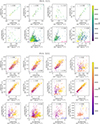 |
Fig. A.1. Correlations between energy bands for Mrk 421 (top) and Mrk 501 (bottom), where r is the Pearson correlation coefficient. There are strong correlations within the optical and UV bands. If considering the entire period there are no correlations between the optical/UV and X-ray bands, but some do appear when the X-rays are divided into hard and soft states. |
All Tables
All Figures
|
Fig. 1. Multi-wavelength light curves of Mrk 421 UV, Mrk 421 X-ray, Mrk 501 optical, Mrk 501 UV, and Mrk 501 X-ray. The legend shows the Swift telescope and filter used to collect the data, as well as the number of observations in each band. Each data point represents one observation. We present the full dynamic range of the data, in linear scaling, and observe higher variability at higher frequencies. |
| In the text | |
|
Fig. 2. Flux distributions for, from left to right, Mrk 421 UV, Mrk 421 X-ray, Mrk 501 UV, and Mrk 501 X-ray. The skewness parameter, γ, a metric of lognormality, is shown in the legend and increases with photon energy. |
| In the text | |
|
Fig. 3. X-ray log parabola fit parameters, α and β, as a function of flux. Mrk 421 (top) and Mrk 501 (bottom) follow the harder-when-brighter trend, with no trend in curvature. |
| In the text | |
|
Fig. 4. Structure functions for Mrk 421 UV (far left), Mrk 421 X-ray (centre left), Mrk 501 UV (centre right), and Mrk 501 X-ray (far right). After 2000 days these are badly affected by systematics, so peaks right of this value should not be trusted. Only Mrk 421 X-ray appears to reach saturation. |
| In the text | |
|
Fig. 5. Lomb-Scargle periodograms for Mrk 421 UV (top left), Mrk 421 X-ray (top right), Mrk 501 UV (bottom left), and Mrk 501 X-ray (bottom right). Only the latter contains a peak above the 3σ significance level, which falls at around 400 days. |
| In the text | |
|
Fig. 6. Discrete auto-correlation functions for Mrk 421 UV (top left), Mrk 421 X-ray (top right), Mrk 501 UV (bottom left), and Mrk 501 X-ray (bottom right). Again only the latter contains any points above the 3σ significance level, at around 1400 days. |
| In the text | |
|
Fig. 7. UV vs X-ray discrete cross-correlation functions for Mrk 421 (top) and Mrk 501 (bottom). |
| In the text | |
|
Fig. A.1. Correlations between energy bands for Mrk 421 (top) and Mrk 501 (bottom), where r is the Pearson correlation coefficient. There are strong correlations within the optical and UV bands. If considering the entire period there are no correlations between the optical/UV and X-ray bands, but some do appear when the X-rays are divided into hard and soft states. |
| In the text | |
Current usage metrics show cumulative count of Article Views (full-text article views including HTML views, PDF and ePub downloads, according to the available data) and Abstracts Views on Vision4Press platform.
Data correspond to usage on the plateform after 2015. The current usage metrics is available 48-96 hours after online publication and is updated daily on week days.
Initial download of the metrics may take a while.