| Issue |
A&A
Volume 706, February 2026
|
|
|---|---|---|
| Article Number | A44 | |
| Number of page(s) | 9 | |
| Section | Stellar structure and evolution | |
| DOI | https://doi.org/10.1051/0004-6361/202557649 | |
| Published online | 30 January 2026 | |
The intermediate neutron capture process
VI. Proton ingestion and i-process in rotating magnetic asymptotic giant branch stars
1
Institut d’Astronomie et d’Astrophysique, Université Libre de Bruxelles, CP 226 B-1050 Brussels, Belgium
2
BLU-ULB, Brussels Laboratory of the Universe, blu.ulb.be Brussels, Belgium
3
Département d’Astronomie, Université de Genève Chemin Pegasi 51 1290 Versoix, Switzerland
4
Yunnan Observatories, Chinese Academy of Sciences Kunming 650216, China
★ Corresponding author: This email address is being protected from spambots. You need JavaScript enabled to view it.
Received:
10
October
2025
Accepted:
20
December
2025
Abstract
Context. The intermediate neutron-capture process (i-process) can occur during proton ingestion events (PIEs), which may take place in the early evolutionary phases of asymptotic giant branch (AGB) stars.
Aims. We investigate the impact of rotational and magnetic mixing on i-process nucleosynthesis in low-metallicity, low-mass AGB stars.
Methods. We computed AGB models with [Fe/H] = −2.5 and −1.7 and initial masses of 1 and 1.5 M⊙ using the STAREVOL code, including a network of 1160 nuclei coupled to transport equations. Rotating models incorporate a calibrated Tayler-Spruit (TS) dynamo to account for core rotation rates inferred from asteroseismic observations of solar-metallicity sub-giants and giants. Initial rotation velocities of 0, 30, and 90 km s−1 were considered, along with varying assumptions for magnetic mixing.
Results. Rotation without magnetic fields strongly suppresses the i-process due to the production of primary 14N, which is subsequently converted into 22Ne – a potent neutron poison during the PIE. Including magnetic fields via the TS dynamo restores the models close to their non-rotating counterparts: strong core-envelope coupling suppresses shear mixing and prevents primary 14N synthesis, yielding i-process nucleosynthesis similar to non-rotating models. We also find that rotational mixing during the AGB phase is insufficient to affect the occurrence of PIEs.
Conclusions. Proton ingestion event-driven nucleosynthesis proceeds similarly in asteroseismic-calibrated magnetic rotating AGB stars and non-rotating stars, producing identical abundance patterns.
Key words: asteroseismology / nuclear reactions / nucleosynthesis / abundances / stars: AGB and post-AGB / stars: interiors / stars: magnetic field / stars: rotation
© The Authors 2026
 Open Access article, published by EDP Sciences, under the terms of the Creative Commons Attribution License (https://creativecommons.org/licenses/by/4.0), which permits unrestricted use, distribution, and reproduction in any medium, provided the original work is properly cited.
This article is published in open access under the Subscribe to Open model. This email address is being protected from spambots. You need JavaScript enabled to view it. to support open access publication.
1. Introduction
Understanding the chemical evolution of the Universe requires identifying the nucleosynthetic processes and their astrophysical sites. Elements heavier than iron are mainly produced through the slow (s) and rapid (r) neutron-capture processes, which occur at neutron densities of Nn ∼ 105 − 1010 and Nn > 1020 cm−3, respectively (e.g. Arnould & Goriely 2020). The s-process primarily takes place in asymptotic giant branch (AGB) stars and in the helium-burning cores of massive stars (e.g. Lugaro et al. 2023, and references therein), while the r-process is associated with more extreme environments such as neutron star mergers, collapsars, or magnetorotational supernovae (e.g. Arnould et al. 2007; Wanajo et al. 2014; Siegel et al. 2019).
In addition to the s- and r-processes, an intermediate neutron-capture process (i-process) has been proposed (Cowan & Rose 1977), operating at neutron densities of Nn ∼ 1013 − 1016 cm−3. Its existence is supported by stars showing chemical abundance patterns inconsistent with either the s- or r-process alone, but well reproduced by i-process models (r/s stars; e.g. Mishenina et al. 2015; Roederer et al. 2016; Karinkuzhi et al. 2021; Hansen et al. 2023). Evidence for proton ingestion and i-process nucleosynthesis may also be present in the Sakurai object (Asplund et al. 1999; Herwig et al. 2011) and in certain pre-solar grains (Fujiya et al. 2013; Liu et al. 2014; Choplin et al. 2024a).
The i-process can be triggered when protons are ingested into a convective helium-burning zone. This is expected in several astrophysical sites (see Choplin et al. 2021, for a detailed list), notably low-metallicity, low-mass AGB stars (e.g. Iwamoto et al. 2004; Cristallo et al. 2009; Suda & Fujimoto 2010; Ritter et al. 2018; Choplin et al. 2022a). The proton ingestion event (PIE) mechanism is illustrated in Fig. 1. During a PIE, at the beginning of the thermally pulsing AGB phase, protons are mixed into the convective thermal pulse, captured through 12C(p, γ)13N, and rapidly converted to 13C via β-decay. The subsequent 13C(α, n)16O reaction at ∼250 MK produces neutron densities up to Nn ∼ 1015 cm−3, triggering an i-process nucleosynthesis and potentially leading to actinide production (Choplin et al. 2022b). After the neutron density peak (green zone in Fig. 1), the i-process material is rapidly mixed throughout the entire thermal pulse, before it splits (at Mr ≃ 0.52 and model ≃90235 in Fig. 1). The processed material is ultimately dredged into the envelope and expelled through stellar winds.
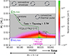 |
Fig. 1. Kippenhahn diagram illustrating key features of a PIE in a non-rotating 1 M⊙, [Fe/H] = −2.5 AGB model, computed with the STAREVOL code. Grey regions indicate convective zones. The dashed green (blue) line marks the location of maximum H-burning (He-burning) energy. The colour map shows the neutron density. The time between the peak neutron density and the split is Δt1 ≃ 100 h, while the total duration of the sequence shown is Δt2 ≃ 0.1 yr. |
Most AGB star models do not include rotation, although such stars as AGBs do rotate (e.g. Vlemmings et al. 2018). Rotation affects stellar evolution by distorting the stellar surface at high speeds and by driving instabilities that transport angular momentum (AM) and chemical elements (e.g. Heger et al. 2000; Maeder & Meynet 2012). Early studies suggested that rotational mixing could create a 13C-pocket (Langer et al. 1999). However, detailed models showed that the pocket was too small to reproduce observed s-process enrichments and that extra 14N synthesized thanks to rotation acts as a neutron poison, quenching s-process efficiency (Herwig et al. 2003; Siess et al. 2003, 2004). Later, Piersanti et al. (2013) computed yields for rotating AGB stars and confirmed that rotation leads to the contamination of the 13C-pocket by the poisonous 14N. However, varying the initial rotation rates (10 − 120 km s−1) and mixing efficiencies, they showed that a wide range of abundance patterns can be obtained.
Asteroseismic studies of sub-giant and red giant stars have revealed their internal and envelope rotation rates (e.g. Beck et al. 2012; Deheuvels et al. 2012, 2020; Mosser et al. 2012; Di Mauro et al. 2016; Triana et al. 2017; Gehan et al. 2018; Tayar et al. 2019; Li et al. 2024; Mosser et al. 2024; Dhanpal et al. 2025). Comparisons with rotating models that include only AM transport by hydrodynamic instabilities provide too little coupling between the core and the envelope to reproduce the observed core rotation rates (Eggenberger et al. 2012; Marques et al. 2013; Ceillier et al. 2013; Tayar & Pinsonneault 2013; Cantiello et al. 2014; Eggenberger et al. 2017, 2019; Moyano et al. 2022). This demonstrates that at least one additional, efficient AM transport mechanism is missing in the radiative zones of red giants. To match observed core rotation rates, den Hartogh et al. (2019) introduced an artificial, constant viscosity term in their solar metallicity, 2 M⊙ rotating AGB models. They found that s-process production remained similar to non-rotating cases due to the strong reduction of rotationally induced mixing.
Motivated by the work of Fuller et al. (2019), Eggenberger et al. (2022) proposed a modified version of the Tayler-Spruit (TS) dynamo (Spruit 2002) able to reproduce asteroseismic observations of sub-giant and red giant stars. This calibrated version better matches the core and surface rotation of low-mass (1.4 − 2 M⊙) Gamma Doradus pulsators (Moyano et al. 2023a) than models without magnetic fields (Ouazzani et al. 2019). Surface boron abundances in massive stars are also better accounted for when including the modified TS dynamo (Asatiani et al. 2025).
This study is the first to investigate the impact of rotation on i-process nucleosynthesis in AGB stars. To account for the asteroseismic constraints available for red giant stars, we implemented the modified TS dynamo proposed by Eggenberger et al. (2022). Sect. 2 describes the models and physical ingredients, while Sect. 3 discusses the calibration of the dynamo. Results are presented in Sects. 4 and 5, and conclusions are summarized in Sect. 6.
2. Physical inputs of the models
The stellar models were computed with the STAREVOL code (Siess et al. 2000; Siess 2006; Goriely & Siess 2018, and references therein). As a first step, 1.1 M⊙ solar-metallicity models were computed to calibrate rotational mixing efficiency (Sect. 3). Then, 1 and 1.5 M⊙ models at [Fe/H] = −2.5 and −1.7, with 0 < vini < 90 km s−1 and varying strengths of magnetic mixing (controlled by the constant CT; see Eq. (8) in Sect. 2.2 and Table 1) were computed. The solar(-scaled) composition was taken from Asplund et al. (2009). Mass loss was treated using the prescription from Schröder & Cuntz (2007) up to the AGB phase and from Vassiliadis & Wood (1993) thereafter. As in previous studies, opacity variations due to molecular formation were included once the star became carbon-rich (Marigo 2002). A mixing-length parameter of 1.75 was adopted. Nuclear burning was followed with a 411-isotope network (from 1H to 211Po) up to the onset of a PIE, at which point we switched to an i-process network of 1160 isotopes (from 1H to 253Cf) coupled with transport equations. Convective overshooting was included from the AGB phase onwards, at the top of thermal pulses (Sect. 2.4). For additional details on the physical inputs, especially the nuclear reaction networks and reaction rates, we refer to Choplin et al. (2021, 2022a) and Goriely et al. (2021).
Main characteristics of the models computed in this work.
Proton ingestion events generally occur during the first thermal pulses, dredging metals to the AGB surface and thereby increasing opacity and mass loss (e.g. Sect. 3.3 in Choplin et al. 2022a). For the low initial masses considered here (1 − 1.5 M⊙), this results in rapid envelope loss, premature termination of the thermal pulse AGB phase, and suppression of s-process nucleosynthesis, which is thus not addressed in this study.
2.1. Transport of angular momentum
Angular momentum transport is solved simultaneously with stellar structure equations. The equation for AM transport is purely diffusive and can be written as
![Mathematical equation: $$ \begin{aligned} \frac{\partial r^{2}\Omega }{\partial t} = \frac{\partial }{\partial m_r} \left[\left(4\pi r^{2} \rho \right)^{2} D_{\rm ang} \, r^{2}\frac{\partial \Omega }{\partial m}\right], \end{aligned} $$](/articles/aa/full_html/2026/02/aa57649-25/aa57649-25-eq1.gif) (1)
(1)
with
 (2)
(2)
where Dconv is the diffusion coefficient due to convection (derived from the mixing-length theory), Dover the overshoot coefficient (see Sect. 2.4), and Dshear the secular shear coefficient from Maeder (1997), which can be expressed as (Meynet et al. 2013)
 (3)
(3)
with Hp being the pressure scale height, K the thermal diffusivity,  ,
,  , ∇, ∇ad, and ∇μ the temperature, adiabatic, and mean molecular weight gradients, respectively. The Dmag coefficient in Eq. (2) denotes the viscosity associated with AM transport by the Tayler instability described in Sect. 2.3.
2.2. Transport of chemicals
The abundance Xi of a nucleus i is followed by solving the diffusive and nuclear burning reaction equation
![Mathematical equation: $$ \begin{aligned} \frac{\partial X_i}{\partial t} = \frac{\partial }{\partial m_r} \left[\,(4 \pi r^2 \rho )^2\,D_{\rm chem}\, \frac{\partial X_i}{\partial m_r}\right] + \frac{\partial X_i}{\partial t}\bigg |_{\rm nuc}, \end{aligned} $$](/articles/aa/full_html/2026/02/aa57649-25/aa57649-25-eq6.gif) (4)
(4)
where
 (5)
(5)
with Dconv, Dover, and Dshear as in Sect. 2.1 and Deff the effective mixing coefficient from Chaboyer & Zahn (1992),
 (6)
(6)
where U(r) is the amplitude of the radial component of the meridional velocity (Maeder & Zahn 1998) and Dh the horizontal (i.e. on an isobaric surface) shear diffusion coefficient from Zahn (1992). The Dh coefficient can be expressed as
 (7)
(7)
with  and ch = 1,
  being the average value of Ω on an isobar and V the horizontal component of the meridional circulation.
The first and second terms on the right-hand side of Eq. (4) account for the changes resulting from diffusive transport and nuclear burning, respectively. During a PIE, the convective and nuclear burning timescales become similar (about 1 h), requiring nucleosynthesis and transport of chemical species to be solved simultaneously (cf. Sect. 2.1 in Choplin et al. 2022a). Unlike AM, no magnetic term is included for the transport of chemicals (Eq. 5) because the chemical mixing caused by the Tayler instability is likely negligible (Fuller et al. 2019).
2.3. Asteroseismic-calibrated version of the Tayler-Spruit dynamo
Following Eggenberger et al. (2022), the Dmag coefficient in Eq. (2) can be written as
 (8)
(8)
with  the shear parameter, Neff the effective Brunt-Väisälä frequency given by
 (9)
(9)
where NT and Nμ denote the thermal and chemical composition components of the Brunt–Väisälä frequency, and η the magnetic diffusivity. The CT quantity is a dimensionless calibration parameter accounting for uncertainties in the damping timescale of the azimuthal magnetic field. The n parameter distinguishes between different prescriptions: the original TS dynamo corresponds to n = 1, CT = 1, while n = 3, CT = 1 recovers the prescription of Fuller et al. (2019). The asteroseismic calibration of Eggenberger et al. (2022) instead adopts n = 1 and CT = 216 and reproduces the core rotation rates of red giants (thick solid blue line in Fig. 2). We implemented the general TS formalism of Eggenberger et al. (2022) in STAREVOL, using different versions that vary the CT value (see Sect. 3). The dynamo operates only when the shear parameter q exceeds a critical threshold value qmin required for the magnetic instability to develop. This minimum threshold can be expressed as (Eq. 12 in Eggenberger et al. 2022):
 (10)
(10)
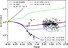 |
Fig. 2. Surface (dashed lines, Ωs) and core (solid lines, Ωc) rotation rates as a function of surface gravity for 1.1 M⊙, solar-metallicity models with vini = 5 km s−1. Models are computed without (black) and with the Tayler instability, using n = 1 and various values of the calibration constant CT (green, red, and blue). The thick blue lines show the surface and core rotation of the 1.1 M⊙, solar-metallicity model from Eggenberger et al. (2022) (E22) computed with GENEC (n = 1, CT = 216). Large black-filled (open) symbols indicate observed surface (core) rotation rates of sub-giant stars (Deheuvels et al. 2014), while the smaller black dots show core rotation rates of RGB stars (Gehan et al. 2018). |
2.4. Convective overshooting
The prescription of Goriely & Siess (2018) was used for convective overshooting. The overshoot diffusion coefficient, Dover, follows the expression
 (11)
(11)
where z* = fover Hp ln(Dcb)/2 is the distance over which mixing occurs, Dmin is the value of the diffusion coefficient at the boundary z = z*, and p and fover are free parameters. Below Dmin, it was assumed that Dover = 0. Choplin et al. (2024b) have extensively studied the impact of these overshoot parameters on the development of PIE and i-process nucleosynthesis in AGB stars. It was shown that convective overshooting at the top of the thermal pulse can trigger PIEs in higher-mass, higher-metallicity AGB stars. Here we considered convective overshooting at the top of the thermal pulse only and adopted fover = 0.04, Dmin = 1 cm2 s−1 and p = 1 in all models (these are the standard values used in Choplin et al. 2024b).
3. Asteroseismic-calibrated version of the Tayler-Spruit dynamo
To calibrate the modified TS dynamo of Eggenberger et al. (2022), we computed 1.1 M⊙ solar-metallicity models (Z = 0.0134) with STAREVOL, adopting vini = 5 km s−1 (as in Eggenberger et al. 2022) and testing CT = 0 (no AM transport by magnetic fields), 1 (original TS dynamo), 50, and 216. The surface rotation of all models (dashed black line in Fig. 2) agrees with the observed sub-giant velocities of Deheuvels et al. (2014, filled black symbols) and follows a similar evolution to the Eggenberger et al. (2022) reference model, computed with the GENEC stellar evolution code (dashed blue line).
The core rotation rates of sub-giants and giants inferred from asteroseismology are reproduced only by our magnetic models with CT = 50 (red line) and, to a lesser extent, CT = 216 (thin solid blue line). From log g ≃ 3.75, our CT = 216 model rotates about twice as slowly as the Eggenberger et al. (2022) model (thick solid blue line), whereas the CT = 50 case recovers their reference track. These discrepancies likely stem from differences in the input physics between GENEC and STAREVOL (e.g. advective vs diffusive treatment of AM transport), whose detailed origin is beyond the scope of this work. Overall, this calibration step confirms that STAREVOL models can reproduce the observed core rotation rates of giants when adopting the generalized TS formalism.
In the following, we examine low-metallicity 1 and 1.5 M⊙ models (Table 1) with CT = 0 (non-magnetic), 1, 50, and 216. Current asteroseismic constraints do not indicate any significant dependence of CT on stellar mass (e.g. Fig. 3 of Eggenberger et al. 2022), and the available observations at nearly solar metallicity reveal no clear trend with metallicity. However, since no constraints exist at the low metallicities relevant for this work, exploring different values of CT remains justified.
4. Rotational mixing and proton ingestion events
In magnetic models (CT > 0), core-envelope coupling transfers AM outwards, causing the core rotation rate to steadily decrease rather than rise, as in non-magnetic rotating models. Figure 3 shows the angular velocity profiles of 1.0 M⊙, [Fe/H] = −2.5 models with vini = 30 km s−1 at the beginning of the red giant branch (RGB) for different values of CT. The non-magnetic case (black) exhibits strong core-envelope differential rotation (∼5 dex), while in magnetic models the coupling strengthens with increasing CT, leading to progressively slower core rotation rates.
 |
Fig. 3. Angular velocity profiles for rotating 1.0 M⊙, [Fe/H] = −2.5 models for various values of CT. The structure corresponds to the moment when the convective envelope reaches its deepest extent during the first dredge-up. |
At fixed initial mass and metallicity, our models show comparable evolution through the main-sequence, RGB, and AGB phases, with similar thermal pulse properties and envelope masses, independently of the values of CT and vini. For example, in our seven [Fe/H] = −2.5 models, PIEs occur under nearly identical conditions and lead to similar i-process nucleosynthesis, except in the non-magnetic rotating case (M1.0z2.5_v30; see Sect. 5.2.1).
Importantly, we find that rotational mixing is too weak in all our rotating models to trigger the occurrence of PIEs on its own. As an example, we considered the M1.0z1.7_v90_CT216 model during the first thermal pulse and switched off overshooting, leading to no PIE occurring1. At the pulse maximum extent, the distance between the top of the convective pulse and the first H-rich layer (XH > 10−3) is r = 0.032 R⊙. With a pulse duration of τ ∼ 400 yr, the diffusion coefficient needed to connect the H-rich layers to the convective zone is D ∼ r2/τ ∼ 4 × 108 cm2 s−1 – several orders of magnitude higher than the typical Dshear in magnetic rotating models (Fig. 4, middle and right panels). Non-magnetic models are also far from these values, especially in the zone of interest, i.e. below the H-rich layers (left panel). This demonstrates that rotation-induced mixing during the AGB phase is insufficient to trigger PIEs by itself.
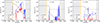 |
Fig. 4. Diffusion coefficients Dshear and Deff between the convective thermal pulse and envelope, just prior to the PIE for 1 M⊙, [Fe/H] = −2.5, vini = 30 km s−1 models with CT = 0 (no TS dynamo), CT = 50, and CT = 216. The profiles of angular velocity (Ω) and hydrogen mass fraction (XH, scaled by 109 and 103, respectively) are also shown. Grey- and orange-shaded areas indicate convective and overshoot zones, respectively. |
5. Impact of rotation on i-process nucleosynthesis and Fluorine synthesis
5.1. The dilution procedure
To estimate the surface abundances resulting from i-process nucleosynthesis in our 1 M⊙, [Fe/H] = −2.5 AGB models, we adopted the dilution procedure described in Martinet et al. (2024, Sect. 3.1). During a PIE, heavy-element nucleosynthesis occurs prior to the splitting of the convective pulse (Choplin et al. 2022a, 2024b). Since the post-split evolution (including mixing with the convective envelope) does not substantially alter these abundances, a computationally efficient approach was employed: the mean abundances of each element in the upper part of the convective pulse, just after the split, were diluted into the convective envelope using a fixed dilution factor calibrated on a full non-rotating 1 M⊙, [Fe/H] = −2.5 AGB model. Because the effect of rotation on the structure is small (Sect. 4), this calibration can be safely used in our rotating models – except for the M1.0z2.5_v30 model, however, which behaves differently during the PIE (Sect. 5.2.1). This method yields accurate approximations of the final surface abundances without the need to evolve the model through the complete envelope mixing phase. For more details on the implementation and accuracy of this method, we refer to Sect. 3.1 of Martinet et al. (2024).
5.2. The [Fe/H] = –2.5 models
During the PIE, our [Fe/H] = −2.5 models reach peak neutron densities in the range 8.1 × 10¹³ < Nn, max < 8.5 × 1014 cm−3 (Table 1). Despite this variation, all models – except M1.0z2.5_v30 (see Sect. 5.2.1) – undergo very similar i-process nucleosynthesis (Fig. 5).
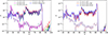 |
Fig. 5. Mass fractions of heavy elements in the convective thermal pulse, just before (dotted lines) and after (solid lines) the main proton ingestion for our 1 M⊙, [Fe/H] = −2.5 models. Left panel: Non-rotating model (black) and models with vini = 30 km s−1 and CT = 0 (magenta), 1 (green), 50 (red), and 216 (blue). Right panel: Non-rotating model (black) and models with vini = 90 km s−1 and CT = 50 (red) and 216 (blue). |
The i-process converts mostly Fe – whose mass fraction drops from 4 × 10⁻⁶ before the PIE to ∼10−7 after in the convective pulse – into heavier elements. Most trans-iron elements increase by 3 − 4 dex (Fig. 5), with significant production of Sr (Z = 38), Zr (Z = 40), Sn (Z = 50), Xe (Z = 54), Cs (Z = 55), Ba (Z = 56), and Pb (Z = 82). The processed material is subsequently diluted into the convective envelope, enriching the AGB surface; the final [X/Fe] ratios are shown in Fig. 6 (top panel). In most models, actinide production (especially Th and U) remains low because convective overshooting, included in all our models, was shown to slightly weaken the i-process, limiting the synthesis of actinides (Choplin et al. 2024b). An exception is the M1.0z2.5_v30_CT50 model, which reaches the highest neutron density (8.5 × 1014 cm−3) and produces [Th/Fe] = 0.61 and [U/Fe] = 1.44 (Fig. 6, top panel).
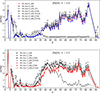 |
Fig. 6. Final surface [X/Fe] ratios after the PIE for our [Fe/H] = −2.5 (top) and [Fe/H] = −1.7 (bottom) models. |
5.2.1. The poisoning effect of primary 22Ne on i-process nucleosynthesis
Although its peak neutron density is comparable to that of other [Fe/H] = −2.5 models (Table 1), the M1.0z2.5_v30 model experiences only a very weak i-process during the PIE, which occurs during the very first TP. As a result, it exclusively produces elements with Z < 40, resembling a convective s-process nucleosynthesis (magenta pattern in the left panel of Fig. 5). The reason for this is discussed below.
After the main-sequence and RGB phases, our models undergo helium flash, which ignites off-centre at Mr ≃ 0.2 M⊙ due to neutrino losses. A large convective zone (Mr ≃ 0.2 − 0.5 M⊙) forms, producing significant amounts of 12C from 4He. Once this convective zone recedes, He burning continues in the core, leaving a 12C-rich radiative layer beneath the H-burning shell. In the M1.0z2.5_v30 model, rotational mixing mixes 12C into the H-burning shell, boosting the CNO cycle and generating primary214N and 13C. During the subsequent evolution, when the He-burning shell moves through 14N-rich layers, 22Ne is massively produced by 14N(α, γ)18F(β+)18O(α, γ)22Ne. Just before the first thermal pulse (where a PIE occurs), the 22Ne mass fraction peaks at 1.7 × 10⁻² in M1.0z2.5_v30, compared with ≲5 × 10⁻⁵ in other [Fe/H] = −2.5 models. During the PIE, 22Ne(n, γ) reaction has among the strongest fluxes and acts as a severe poison. It results in a weak i-process that synthesizes mainly elements with Z < 40 (Figs. 5 and 6). Consequently, the final surface Ne abundance is high in this model (Fig. 6, top panel).
The 22Ne(n, γ) reaction competes with 22Ne(p, γ), for which we adopted the rate of Longland et al. (2010). Recently, Lennarz et al. (2020) derived a new experimental rate for the latter reaction, which is higher by a factor of ∼3 compared to Longland et al. (2010) at He-burning temperatures. As a test, we recomputed the M1.0z2.5_v30 model during the PIE using the 22Ne(p, γ) rate increased by a factor of three. We find that such an enhancement leads to an overproduction by a factor of ∼2 − 3 of elements with 30 < Z < 40 in the thermal pulse after the PIE.
In the non-rotating [Fe/H] = −2.5 model, no additional 22Ne is produced because mixing is absent. In magnetic rotating models, the TS dynamo flattens the angular velocity profile (Fig. 3), which greatly suppresses shear mixing–the main driver of chemical transport in non-magnetic rotating models–since it depends on the gradient of Ω (Eq. 3). Consequently, final surface Ne (Z = 10) abundances remain much lower in both non-rotating and magnetic models (Fig. 6, top panel).
5.2.2. Fluorine and Sodium synthesis during the PIE of the M1.0z2.5_v30 model
The M1.0z2.5_v30 model undergoes a weak i-process (Sect. 5.2.1) but is the only model that produces significant Fluorine ([F/Fe] ≃ 2.5, Fig. 6). The 19F isotope originates from primary 14N synthesized prior to the AGB phase (Sect. 5.2.1) through four roughly equally important reaction chains:
-
14N(α, γ)18F(n, α)15N(α, γ)19F,
-
14N(α, γ)18F(β+)18O(p, α)15N(α, γ)19F,
-
14N(α, γ)18F(n, p)18O(p, α)15N(α, γ)19F,
-
14N(α, γ)18F(β+)18O(n, γ)19O(β−)19F.
Because of the high neutron density, the reaction 19F(n, γ)20F is also efficient, causing partial destruction of 19F. However, the net outcome remains a substantial production of 19F.
Sodium is also efficiently produced in this model ([Na/Fe] ≃ 1.5, Fig. 6) through the reaction chain 22Ne(n, γ)23Ne(β−)23Na, with most of the 22Ne originating from the primary 14N synthesized earlier (Sect. 5.2.1). Thus, substantial F, Ne, and Na production during PIEs requires prior synthesis of primary 14N. This occurs only in our rotating, non-magnetic model, which is disfavoured by asteroseismic constraints (Fig. 2), even though no asteroseismic observations exist at such low metallicities.
5.3. The [Fe/H] = –1.7 models
As for the [Fe/H] = −2.5 models, including rotation and magnetic fields in the [Fe/H] = −1.7 models results in evolution and nucleosynthesis (Figs. 6 and 7) nearly identical to the non-rotating cases. Overall surface enrichment is lower in the 1.5 M⊙ models than in the 1 M⊙ models, because the PIE products are diluted into a more massive convective envelope (∼0.2 vs ∼0.7 M⊙, respectively).
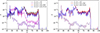 |
Fig. 7. Same as Fig. 5, but for the [Fe/H] = −1.7 models with Mini = 1.0 M⊙ (left panel) and 1.5 M⊙ (right panel). Models without rotation (black), with vini = 30 km s−1 (magenta), with vini = 90 km s−1 and CT = 50 (red) and with vini = 90 km s−1 and CT = 216 (blue) are shown. |
The rotating non-magnetic M1.0z1.7_v30 model undergoes a weaker i-process nucleosynthesis (bottom panel of Fig. 6, and left panel of Fig. 7) for the same reasons as the M1.0z2.5_v30 model (Sect. 5.2.1). However, compared to the M1.0z2.5_v30 model (Fig. 6), a larger amount of heavy elements is produced because the PIE develops during the third rather than the first thermal pulse, as in the lower metallicity model. Although the 22Ne abundance during the PIE is similar in both cases, most of the primary 14N is consumed in the two preceding TPs, thereby reducing its poisoning effect and allowing for more efficient synthesis of heavy elements.
Another difference is that, unlike the M1.0z2.5_v30 model, no fluorine enhancement is noticed at the surface of the M1.0z1.7_v30 model (Fig. 6, bottom panel). Owing to the large amount of primary 14N synthesized prior to the AGB phase, 19F is efficiently produced during the first two TPs (where no PIE occurs) through the reaction chain 14N(α, γ)18F(β+)18O(p, α)15N(α, γ)19F with protons supplied by 14N(n, p)14C. At this stage, the neutron flux is too low to significantly destroy 19F via the 19F(n, γ)20F channel. But the 19F synthesized during these first two TPs does not reach the stellar surface because the third dredge-ups are not deep enough. During the subsequent third TP, when the PIE takes place, the production of 19F becomes inefficient because only a small amount of 14N remains. Instead, the destruction channel 19F(n, γ)20F strongly dominates, ultimately leading to the nearly complete depletion of 19F. Hence, efficient fluorine production requires not only prior synthesis of primary 14N but also that the PIE occurs during the very first TP.
6. Conclusions
In this study, we explored the effect of rotation on i-process nucleosynthesis in AGB stars. To incorporate constraints from asteroseismic observations, we implemented in STAREVOL a modified version of the TS dynamo, as recently proposed by Eggenberger et al. (2022), designed to reconcile rotating models with observational data available for red giant stars. We computed both classical rotating models (without the dynamo) and magnetic rotating models (with the dynamo).
We found that i-process nucleosynthesis is strongly suppressed in rotating AGB models that employ the classical treatment of AM transport based purely on hydrodynamical processes and no magnetic fields (Zahn 1992). This is due to the production of primary 14N prior to the AGB phase, which is subsequently converted into 22Ne that acts as a strong neutron poison during the PIE via the 22Ne(n, γ) reaction. As a result, only elements with Z < 40 are synthesized, and their enhancement is modest ([X/Fe] < 1 dex). In addition, rotational mixing alone can lead to significant production of fluorine and sodium during the PIE through four reaction chains originating from 14N. However, efficient fluorine synthesis occurs only if the PIE develops during the very first thermal pulse.
In contrast, in rotating magnetic models, strong core-envelope coupling suppresses shear mixing, preventing production of primary 14N and the associated excess of 22Ne. Consequently, i-process nucleosynthesis in these models closely mirrors those of non-rotating stars. This behaviour is largely independent of the rotation rate or the strength of the TS dynamo (parametrized by CT) and is consistent across different metallicities ([Fe/H] = −2.5 and −1.7) and initial masses (1 and 1.5 M⊙). Although overshooting is crucial for initiating PIEs (especially at higher masses and metallicities Choplin et al. 2024b), we find that rotational mixing during the AGB phase is too weak to affect their occurrence.
Internal magnetic fields generated by the TS dynamo can help reconcile models with asteroseismic observations, but they cannot fully explain the missing AM transport in stars by adopting a single value for the calibration parameter. The internal rotation profiles of, for example, γ Doradus stars (Moyano et al. 2024) and white dwarfs (den Hartogh et al. 2020) have indeed been shown to be consistent with magnetic models that use a lower value of the TS dynamo calibration parameter than that needed to reproduce the core rotation rates of red giants. Additional processes – such as internal gravity waves (Pinçon et al. 2017), mixed modes (Belkacem et al. 2015; Bordadágua et al. 2025), or azimuthal magneto-rotational instability (Moyano et al. 2023b; Meduri et al. 2024) – could also play a role in the internal transport of AM. These mechanisms could also affect AGB nucleosynthesis and should be investigated in future studies.
Acknowledgments
This work was supported by the Fonds de la Recherche Scientifique-FNRS under Grant No. IISN 4.4502.19. L.S. and S.G. are senior F.R.S-FNRS research associates. A.C. is post-doctorate F.R.S-FNRS fellow. P.E. acknowledges support from the SNF grant No 219745 (Asteroseismology of transport processes for the evolution of stars and planets).
References
- Arnould, M., & Goriely, S. 2020, Progr. Part. Nucl. Phys., 112, 103766 [NASA ADS] [CrossRef] [Google Scholar]
- Arnould, M., Goriely, S., & Takahashi, K. 2007, Phys. Rep., 450, 97 [Google Scholar]
- Asatiani, L., Eggenberger, P., Marchand, M., et al. 2025, A&A, 699, L8 [NASA ADS] [CrossRef] [EDP Sciences] [Google Scholar]
- Asplund, M., Lambert, D. L., Kipper, T., Pollacco, D., & Shetrone, M. D. 1999, A&A, 343, 507 [NASA ADS] [Google Scholar]
- Asplund, M., Grevesse, N., Sauval, A. J., & Scott, P. 2009, ARA&A, 47, 481 [NASA ADS] [CrossRef] [Google Scholar]
- Beck, P. G., Montalban, J., Kallinger, T., et al. 2012, Nature, 481, 55 [Google Scholar]
- Belkacem, K., Marques, J. P., Goupil, M. J., et al. 2015, A&A, 579, A31 [NASA ADS] [CrossRef] [EDP Sciences] [Google Scholar]
- Bordadágua, B., Ahlborn, F., Coppée, Q., et al. 2025, A&A, 699, A310 [NASA ADS] [CrossRef] [EDP Sciences] [Google Scholar]
- Cantiello, M., Mankovich, C., Bildsten, L., Christensen-Dalsgaard, J., & Paxton, B. 2014, ApJ, 788, 93 [Google Scholar]
- Ceillier, T., Eggenberger, P., García, R. A., & Mathis, S. 2013, A&A, 555, A54 [NASA ADS] [CrossRef] [EDP Sciences] [Google Scholar]
- Chaboyer, B., & Zahn, J.-P. 1992, A&A, 253, 173 [Google Scholar]
- Choplin, A., Siess, L., & Goriely, S. 2021, A&A, 648, A119 [NASA ADS] [CrossRef] [EDP Sciences] [Google Scholar]
- Choplin, A., Siess, L., & Goriely, S. 2022a, A&A, 667, A155 [NASA ADS] [CrossRef] [EDP Sciences] [Google Scholar]
- Choplin, A., Goriely, S., & Siess, L. 2022b, A&A, 667, L13 [NASA ADS] [CrossRef] [EDP Sciences] [Google Scholar]
- Choplin, A., Siess, L., & Goriely, S. 2024a, A&A, 691, L7 [NASA ADS] [CrossRef] [EDP Sciences] [Google Scholar]
- Choplin, A., Siess, L., Goriely, S., & Martinet, S. 2024b, A&A, 684, A206 [NASA ADS] [CrossRef] [EDP Sciences] [Google Scholar]
- Cowan, J. J., & Rose, W. K. 1977, ApJ, 212, 149 [Google Scholar]
- Cristallo, S., Piersanti, L., Straniero, O., et al. 2009, PASA, 26, 139 [Google Scholar]
- Deheuvels, S., García, R. A., Chaplin, W. J., et al. 2012, ApJ, 756, 19 [Google Scholar]
- Deheuvels, S., Doğan, G., Goupil, M. J., et al. 2014, A&A, 564, A27 [NASA ADS] [CrossRef] [EDP Sciences] [Google Scholar]
- Deheuvels, S., Ballot, J., Eggenberger, P., et al. 2020, A&A, 641, A117 [EDP Sciences] [Google Scholar]
- den Hartogh, J. W., Hirschi, R., Lugaro, M., et al. 2019, A&A, 629, A123 [NASA ADS] [CrossRef] [EDP Sciences] [Google Scholar]
- den Hartogh, J. W., Eggenberger, P., & Deheuvels, S. 2020, A&A, 634, L16 [NASA ADS] [CrossRef] [EDP Sciences] [Google Scholar]
- Dhanpal, S., Benomar, O., Hanasoge, S., & Fuller, J. 2025, ApJ, 988, 224 [Google Scholar]
- Di Mauro, M. P., Ventura, R., Cardini, D., et al. 2016, ApJ, 817, 65 [NASA ADS] [CrossRef] [Google Scholar]
- Eggenberger, P., Montalbán, J., & Miglio, A. 2012, A&A, 544, L4 [NASA ADS] [CrossRef] [EDP Sciences] [Google Scholar]
- Eggenberger, P., Lagarde, N., Miglio, A., et al. 2017, A&A, 599, A18 [CrossRef] [EDP Sciences] [Google Scholar]
- Eggenberger, P., Deheuvels, S., Miglio, A., et al. 2019, A&A, 621, A66 [NASA ADS] [CrossRef] [EDP Sciences] [Google Scholar]
- Eggenberger, P., Moyano, F. D., & den Hartogh, J. W. 2022, A&A, 664, L16 [NASA ADS] [CrossRef] [EDP Sciences] [Google Scholar]
- Fujiya, W., Hoppe, P., Zinner, E., Pignatari, M., & Herwig, F. 2013, ApJ, 776, L29 [Google Scholar]
- Fuller, J., Piro, A. L., & Jermyn, A. S. 2019, MNRAS, 485, 3661 [NASA ADS] [Google Scholar]
- Gehan, C., Mosser, B., Michel, E., Samadi, R., & Kallinger, T. 2018, A&A, 616, A24 [NASA ADS] [CrossRef] [EDP Sciences] [Google Scholar]
- Goriely, S., & Siess, L. 2018, A&A, 609, A29 [NASA ADS] [CrossRef] [EDP Sciences] [Google Scholar]
- Goriely, S., Siess, L., & Choplin, A. 2021, A&A, 654, A129 [NASA ADS] [CrossRef] [EDP Sciences] [Google Scholar]
- Hansen, T. T., Simon, J. D., Li, T. S., et al. 2023, A&A, 674, A180 [NASA ADS] [CrossRef] [EDP Sciences] [Google Scholar]
- Heger, A., Langer, N., & Woosley, S. E. 2000, ApJ, 528, 368 [NASA ADS] [CrossRef] [Google Scholar]
- Herwig, F., Langer, N., & Lugaro, M. 2003, ApJ, 593, 1056 [NASA ADS] [CrossRef] [Google Scholar]
- Herwig, F., Pignatari, M., Woodward, P. R., et al. 2011, ApJ, 727, 89 [Google Scholar]
- Iwamoto, N., Kajino, T., Mathews, G. J., Fujimoto, M. Y., & Aoki, W. 2004, ApJ, 602, 377 [Google Scholar]
- Karinkuzhi, D., Van Eck, S., Goriely, S., et al. 2021, A&A, 645, A61 [EDP Sciences] [Google Scholar]
- Langer, N., Heger, A., Wellstein, S., & Herwig, F. 1999, A&A, 346, L37 [Google Scholar]
- Lennarz, A., Williams, M., Laird, A. M., et al. 2020, Phys. Lett. B, 807, 135539 [Google Scholar]
- Li, G., Deheuvels, S., & Ballot, J. 2024, A&A, 688, A184 [NASA ADS] [CrossRef] [EDP Sciences] [Google Scholar]
- Liu, N., Savina, M. R., Davis, A. M., et al. 2014, ApJ, 786, 66 [NASA ADS] [CrossRef] [Google Scholar]
- Longland, R., Iliadis, C., Champagne, A. E., et al. 2010, Nucl. Phys. A, 841, 1 [NASA ADS] [CrossRef] [Google Scholar]
- Lugaro, M., Pignatari, M., Reifarth, R., & Wiescher, M. 2023, Annu. Rev. Nucl. Part. Sci., 73, 315 [NASA ADS] [CrossRef] [Google Scholar]
- Maeder, A. 1997, A&A, 321, 134 [NASA ADS] [Google Scholar]
- Maeder, A., & Meynet, G. 2012, Rev. Mod. Phys., 84, 25 [Google Scholar]
- Maeder, A., & Zahn, J.-P. 1998, A&A, 334, 1000 [NASA ADS] [Google Scholar]
- Marigo, P. 2002, A&A, 387, 507 [NASA ADS] [CrossRef] [EDP Sciences] [Google Scholar]
- Marques, J. P., Goupil, M. J., Lebreton, Y., et al. 2013, A&A, 549, A74 [NASA ADS] [CrossRef] [EDP Sciences] [Google Scholar]
- Martinet, S., Choplin, A., Goriely, S., & Siess, L. 2024, A&A, 684, A8 [NASA ADS] [CrossRef] [EDP Sciences] [Google Scholar]
- Meduri, D. G., Jouve, L., & Lignières, F. 2024, A&A, 683, A12 [NASA ADS] [CrossRef] [EDP Sciences] [Google Scholar]
- Meynet, G., Ekstrom, S., Maeder, A., et al. 2013, Lect. Notes Phys., 865, 3 [Google Scholar]
- Mishenina, T., Pignatari, M., Carraro, G., et al. 2015, MNRAS, 446, 3651 [Google Scholar]
- Mosser, B., Goupil, M. J., Belkacem, K., et al. 2012, A&A, 548, A10 [NASA ADS] [CrossRef] [EDP Sciences] [Google Scholar]
- Mosser, B., Dréau, G., Pinçon, C., et al. 2024, A&A, 681, L20 [NASA ADS] [CrossRef] [EDP Sciences] [Google Scholar]
- Moyano, F. D., Eggenberger, P., Meynet, G., et al. 2022, A&A, 663, A180 [NASA ADS] [CrossRef] [EDP Sciences] [Google Scholar]
- Moyano, F. D., Eggenberger, P., Salmon, S. J. A. J., Mombarg, J. S. G., & Ekström, S. 2023a, A&A, 677, A6 [NASA ADS] [CrossRef] [EDP Sciences] [Google Scholar]
- Moyano, F. D., Eggenberger, P., Mosser, B., & Spada, F. 2023b, A&A, 673, A110 [NASA ADS] [CrossRef] [EDP Sciences] [Google Scholar]
- Moyano, F. D., Eggenberger, P., & Salmon, S. J. A. J. 2024, A&A, 681, L16 [NASA ADS] [CrossRef] [EDP Sciences] [Google Scholar]
- Ouazzani, R. M., Marques, J. P., Goupil, M. J., et al. 2019, A&A, 626, A121 [NASA ADS] [CrossRef] [EDP Sciences] [Google Scholar]
- Piersanti, L., Cristallo, S., & Straniero, O. 2013, ApJ, 774, 98 [NASA ADS] [CrossRef] [Google Scholar]
- Pinçon, C., Belkacem, K., Goupil, M. J., & Marques, J. P. 2017, A&A, 605, A31 [NASA ADS] [CrossRef] [EDP Sciences] [Google Scholar]
- Ritter, C., Herwig, F., Jones, S., et al. 2018, MNRAS, 480, 538 [NASA ADS] [CrossRef] [Google Scholar]
- Roederer, I. U., Karakas, A. I., Pignatari, M., & Herwig, F. 2016, ApJ, 821, 37 [Google Scholar]
- Schröder, K. P., & Cuntz, M. 2007, A&A, 465, 593 [NASA ADS] [CrossRef] [EDP Sciences] [Google Scholar]
- Siegel, D. M., Barnes, J., & Metzger, B. D. 2019, Nature, 569, 241 [Google Scholar]
- Siess, L. 2006, A&A, 448, 717 [NASA ADS] [CrossRef] [EDP Sciences] [Google Scholar]
- Siess, L., Dufour, E., & Forestini, M. 2000, A&A, 358, 593 [Google Scholar]
- Siess, L., Goriely, S., & Langer, N. 2003, PASA, 20, 371 [Google Scholar]
- Siess, L., Goriely, S., & Langer, N. 2004, A&A, 415, 1089 [NASA ADS] [CrossRef] [EDP Sciences] [Google Scholar]
- Spruit, H. C. 2002, A&A, 381, 923 [CrossRef] [EDP Sciences] [Google Scholar]
- Suda, T., & Fujimoto, M. Y. 2010, MNRAS, 405, 177 [NASA ADS] [Google Scholar]
- Tayar, J., & Pinsonneault, M. H. 2013, ApJ, 775, L1 [NASA ADS] [CrossRef] [Google Scholar]
- Tayar, J., Beck, P. G., Pinsonneault, M. H., García, R. A., & Mathur, S. 2019, ApJ, 887, 203 [NASA ADS] [CrossRef] [Google Scholar]
- Triana, S. A., Corsaro, E., De Ridder, J., et al. 2017, A&A, 602, A62 [NASA ADS] [CrossRef] [EDP Sciences] [Google Scholar]
- Vassiliadis, E., & Wood, P. R. 1993, ApJ, 413, 641 [Google Scholar]
- Vlemmings, W. H. T., Khouri, T., De Beck, E., et al. 2018, A&A, 613, L4 [NASA ADS] [CrossRef] [EDP Sciences] [Google Scholar]
- Wanajo, S., Sekiguchi, Y., Nishimura, N., et al. 2014, ApJ, 789, L39 [Google Scholar]
- Zahn, J.-P. 1992, A&A, 265, 115 [NASA ADS] [Google Scholar]
Without additional mixing processes (e.g. overshoot), PIEs are expected in AGB models with Mini ≲ 2.5 M⊙ and [Fe/H] < −2 (Fig. 12 in Choplin et al. 2024b).
Synthesized from the initial H and He contents, as opposed to secondary production from the initial metal (elements heavier than He) content.
All Tables
All Figures
|
Fig. 1. Kippenhahn diagram illustrating key features of a PIE in a non-rotating 1 M⊙, [Fe/H] = −2.5 AGB model, computed with the STAREVOL code. Grey regions indicate convective zones. The dashed green (blue) line marks the location of maximum H-burning (He-burning) energy. The colour map shows the neutron density. The time between the peak neutron density and the split is Δt1 ≃ 100 h, while the total duration of the sequence shown is Δt2 ≃ 0.1 yr. |
| In the text | |
|
Fig. 2. Surface (dashed lines, Ωs) and core (solid lines, Ωc) rotation rates as a function of surface gravity for 1.1 M⊙, solar-metallicity models with vini = 5 km s−1. Models are computed without (black) and with the Tayler instability, using n = 1 and various values of the calibration constant CT (green, red, and blue). The thick blue lines show the surface and core rotation of the 1.1 M⊙, solar-metallicity model from Eggenberger et al. (2022) (E22) computed with GENEC (n = 1, CT = 216). Large black-filled (open) symbols indicate observed surface (core) rotation rates of sub-giant stars (Deheuvels et al. 2014), while the smaller black dots show core rotation rates of RGB stars (Gehan et al. 2018). |
| In the text | |
|
Fig. 3. Angular velocity profiles for rotating 1.0 M⊙, [Fe/H] = −2.5 models for various values of CT. The structure corresponds to the moment when the convective envelope reaches its deepest extent during the first dredge-up. |
| In the text | |
|
Fig. 4. Diffusion coefficients Dshear and Deff between the convective thermal pulse and envelope, just prior to the PIE for 1 M⊙, [Fe/H] = −2.5, vini = 30 km s−1 models with CT = 0 (no TS dynamo), CT = 50, and CT = 216. The profiles of angular velocity (Ω) and hydrogen mass fraction (XH, scaled by 109 and 103, respectively) are also shown. Grey- and orange-shaded areas indicate convective and overshoot zones, respectively. |
| In the text | |
|
Fig. 5. Mass fractions of heavy elements in the convective thermal pulse, just before (dotted lines) and after (solid lines) the main proton ingestion for our 1 M⊙, [Fe/H] = −2.5 models. Left panel: Non-rotating model (black) and models with vini = 30 km s−1 and CT = 0 (magenta), 1 (green), 50 (red), and 216 (blue). Right panel: Non-rotating model (black) and models with vini = 90 km s−1 and CT = 50 (red) and 216 (blue). |
| In the text | |
|
Fig. 6. Final surface [X/Fe] ratios after the PIE for our [Fe/H] = −2.5 (top) and [Fe/H] = −1.7 (bottom) models. |
| In the text | |
|
Fig. 7. Same as Fig. 5, but for the [Fe/H] = −1.7 models with Mini = 1.0 M⊙ (left panel) and 1.5 M⊙ (right panel). Models without rotation (black), with vini = 30 km s−1 (magenta), with vini = 90 km s−1 and CT = 50 (red) and with vini = 90 km s−1 and CT = 216 (blue) are shown. |
| In the text | |
Current usage metrics show cumulative count of Article Views (full-text article views including HTML views, PDF and ePub downloads, according to the available data) and Abstracts Views on Vision4Press platform.
Data correspond to usage on the plateform after 2015. The current usage metrics is available 48-96 hours after online publication and is updated daily on week days.
Initial download of the metrics may take a while.