| Issue |
A&A
Volume 706, February 2026
|
|
|---|---|---|
| Article Number | A375 | |
| Number of page(s) | 10 | |
| Section | Stellar structure and evolution | |
| DOI | https://doi.org/10.1051/0004-6361/202557683 | |
| Published online | 20 February 2026 | |
Violent mergers can explain the inflated state of some of the fastest stars in the Galaxy
1
Institut für Physik und Astronomie, Universität Potsdam, Haus 28 Karl-Liebknecht-Str. 24/25 14476 Potsdam-Golm, Germany
2
Max Planck Institut für Astrophysik Karl-Schwarzschild-Straße 1 85748 Garching bei München, Germany
3
Department of Astronomy and Theoretical Astrophysics Center, University of California Berkeley CA 94720-3411, USA
4
Lawrence Livermore National Laboratory Livermore California 94550, USA
5
Center for Astrophysics | Harvard & Smithsonian 60 Garden Street Cambridge MA 02138, USA
★ Corresponding author: This email address is being protected from spambots. You need JavaScript enabled to view it.
Received:
14
October
2025
Accepted:
15
December
2025
Abstract
A significant number of hypervelocity stars with velocities between 1500 − 2500 km s−1 have recently been observed. The only plausible explanation so far is that they were produced through thermonuclear supernovae in white dwarf binaries. Since these stars are thought to be surviving donors of Type Ia supernovae, a surprising finding was that these stars are inflated, with radii an order of magnitude higher than expected for Roche-lobe-filling donors. Recent attempts at explaining them have combined 3D hydrodynamical supernova explosion simulations with 1D stellar modelling to explain the impact of supernova shocks on runaway white dwarfs. However, only the hottest and most compact of those runaway stars can so far marginally be reproduced by detailed models of runaways from supernova explosions. In this and a companion paper, we introduce a new AREPO simulation of two massive CO white dwarfs that explode via a violent merger. During the merger, the primary white dwarf ignites when the secondary is on its last orbit and plunging towards the primary. In the corresponding aftermath, the core of the secondary white dwarf of 0.16 M⊙ remains bound, moving at a velocity of ∼2800 km s−1. We mapped this object into MESA and show that this runaway star can explain the observations of two hypervelocity stars that were dubbed D6-1 and D6-3 based on their original discovery motivated by the D6 scenario, though the violent merger scenario presented here is somewhat distinct from the D6 scenario.
Key words: stars: evolution / stars: kinematics and dynamics / white dwarfs
© The Authors 2026
 Open Access article, published by EDP Sciences, under the terms of the Creative Commons Attribution License (https://creativecommons.org/licenses/by/4.0), which permits unrestricted use, distribution, and reproduction in any medium, provided the original work is properly cited.
This article is published in open access under the Subscribe to Open model. This email address is being protected from spambots. You need JavaScript enabled to view it. to support open access publication.
1. Introduction
Thermonuclear supernovae in white dwarf binaries can leave behind a hypervelocity runaway companion. The discovery of the fastest stars in our Galaxy supports this scenario (Shen et al. 2018a; El-Badry et al. 2023; Hollands et al. 2025). To explain the speeds at which these stars move (1000 − 2500 km s−1), the ‘dynamically driven double-degenerate double-detonation’ (D6) scenario has been invoked. In this scenario, a white dwarf (WD) transfers mass to a more massive white dwarf through dynamically unstable Roche-lobe overflow (Guillochon et al. 2010; Dan et al. 2011, 2012; Pakmor et al. 2013; Shen et al. 2018b); the more massive white dwarf explodes in a Type Ia supernova and leaves the secondary white dwarf behind. In fact, the discovery of the first three stars by Shen et al. (2018a) was considered as a smoking gun for this scenario and provided the motivation to search for them in the first place.
Since then, a total of eight candidate objects for such a scenario are known in the literature. Almost all of them are inflated, having radii of the order of 0.1 R⊙ instead of < 0.01 R⊙, which they would have had as WDs prior to the supernova. Relying on an AREPO 3D hydrodynamical simulation for the detonation phase and a calculation using the 1D stellar-evolution code Modules for Experiments in Stellar Astrophysics (MESA, Paxton et al. 2011, 2013, 2015, 2018, 2019; Jermyn et al. 2023) for the long-term evolution, Bhat et al. (2025) showed that the radii of some of the stars could only be inflated for a few thousand years due to heating by the supernova shock from the primary detonation. This is not enough to explain their observed inflated nature since kinematic ages suggest that stars were formed 0.5 − 3 Myr ago. Recently, Glanz et al. (2025) found an alternative way to make fast and hot hypervelocity stars by the merger disruption of HeCO white dwarfs in binary systems with low-mass carbon-oxygen primary white dwarfs. The donors in this scenario have slightly higher velocities than what would be expected through the D6 scenario, as they are close to being disrupted, significantly overflowing their Roche lobes and plunging towards the primary white dwarf before being ejected. The 1D evolution shows these stars are inflated for times of the order 104 − 106 yr.
While both these efforts can reproduce properties of some of the observed stars, none of them can explain the velocity and inflated nature of the cooler HVWDs (J1235, J1637, and D6 1-3). D6 1-3 in particular were the first three stars to be found. D6-2 is the only one whose properties are in close agreement with a He WD donor scenario (Wong et al. 2024; Shen 2025; Wong & Bildsten 2025), since its velocity is the lowest of all the observed stars. These stars lie in a region (Teff < 9000 K) that none of the long-term evolutionary tracks of the previous simulations reach.
The explanation for the high velocities of these objects in the D6 scenario relies on the assumption that these white dwarfs were Roche-lobe-filling donors in white dwarf binaries. When the accretion starts, unstable mass transfer of 4He, leads to a thermonuclear runaway through dynamical instabilities in the interaction between the accretion stream and the shell of the accretor. When the stream is hot and dense enough, it can detonate the helium shell on the accretor. The shock from this surface detonation propagates and meets at the opposite end of the white dwarf. This shock then traverses inside to compress and consequently ignite carbon (Fink et al. 2007; Guillochon et al. 2010; Kromer et al. 2010; Pakmor et al. 2013; Moll & Woosley 2013; Boos et al. 2021; Pakmor et al. 2022), completely destroying the primary white dwarf. As the timescale on which the primary white dwarf explodes is much shorter than the orbital period of the binary system, the primary suddenly disappears and the secondary white dwarf continues to move with its orbital velocity at this time. However, in the absence of a sufficiently massive helium shell on the primary white dwarf, it may also be possible that the accretor detonates later, when the accretion stream becomes hot and dense enough to drive a carbon detonation directly. This is known as the ‘violent merger’ scenario (Pakmor et al. 2010). Here, the donor is significantly beyond its Roche limit, so the plunging donor star might reach higher velocities than when it fills its Roche lobe. In this case, lower mass donors could have higher velocities, and such disruption detonations could exist for 0.4 M⊙ white dwarfs (Dan et al. 2012). Whether the white dwarfs can come closer to merging and not detonate before that depends on the mass fraction and the 4He shell masses of the two white dwarfs (Shen et al. 2024). If the white dwarfs could come close to merging and the donor could survive the impending supernova explosion, then this would help alleviate some tension between the ejection velocities of the white dwarfs and their masses, since lower mass white dwarfs could also achieve ∼2000 km s−1 velocities.
In this work, we simulated the long-term evolution of a runaway surviving remnant from the violent merger scenario and show that in comparison to the D6 scenario, the runaway can achieve both higher runaway velocity and a more inflated radius for ∼Myr timescales. This paper comes with a companion paper, in which we report on a new 3D hydrodynamical simulation of binary white dwarfs that undergo a supernova explosion and end with a hypervelocity runaway donor remnant. We simulated this using the 3D magneto-hydrodynamic code AREPO (Springel 2010; Pakmor et al. 2016; Weinberger et al. 2020). The simulation followed the evolution until shortly after detonation of the primary white dwarf. We took this surviving donor as input into the 1D, open-source stellar-evolution software MESA. We used the entropy profiles from AREPO to relax and model the subsequent stellar evolution through the following 100 Myr, similarly to what was done in Bhat et al. (2025) and Glanz et al. (2025). In Section 2, we discuss the AREPO simulation. In Section 3, we discuss relaxation in MESA. Section 4 discusses the long-term evolution of the models, and Section 5 compares them to recent observations of hypervelocity stars. We summarise our results in Section 6.
2. 3D hydrodynamical simulation
In this section, we summarise the details of the explosion simulation that produced the bound donor remnant that we then evolved further in MESA. We refer the reader to the companion paper (Pakmor et al. 2025) for a comprehensive explanation of the simulation. We started in AREPO with a double white dwarf system. This simulation starts with the late stages of the inspiral of a binary system of two carbon-oxygen white dwarfs with masses of 1.10 M⊙ and 0.70 M⊙, respectively. The donor model starts with a 50/50 C/O core composition, 0.016 M⊙22Ne, and a 4He shell of 0.0003 M⊙. The secondary has 0.32 M⊙ of carbon, 0.36 M⊙ of oxygen, 0.011 M⊙ of 22Ne, and a He shell of 0.009 M⊙. While helium was accreted in the beginning of the simulation, it is expelled from the system in surface detonation-powered outbursts. Due to the small He shell on the accretor, no coherent helium detonation forms on the primary white dwarf, so the double detonation scenario is avoided. After a few orbits, we artificially decreased the separation to avoid computational costs associated with orbital shrinking. When the white dwarfs are close enough for the secondary to be disrupted, there is almost no 4He left in the system. In the last inspiral of the system, the donor was accelerated towards the accretor. Its impact on the surface of the accretor was enough to create conditions for direct carbon ignition, and the primary white dwarf exploded. The orbital velocity of the donor before it hit the accretor was ∼2700 km s−1.
The accretor exploded completely. In contrast to previous violent merger simulations (Pakmor et al. 2010, 2012; Sato et al. 2015), a small amount of the donor white dwarf (∼0.16 M⊙) remained bound after being hit by the explosion of the primary white dwarf and being burned partially. A small amount of 56Ni and carbon-burning ashes were deposited from the low-velocity tail of the supernova ejecta. Around 1.64 M⊙ of material was ejected in the explosion.
We used AREPO to follow the expanding supernova ejecta and the bound surviving donor star until 1000 s after the explosion. This is of the order of a few dynamical timescales for our slightly expanded runaway,
 (1)
(1)
The final AREPO profile of the remnant that is mapped into MESA contains composition information and averaged 1D temperature-density pairs for different shells of the star. 2D slices of the 3D density structure of the runaway are shown in Figure 1. The total angular momentum and the corresponding averaged rotational velocity are shown in Figure 2. While the inner structure (< 0.05 R⊙) does not deviate more than 10 km s−1 in rotational velocity, the outer part from 0.05 − 0.1 R⊙ has slightly higher rotational-velocity variations, deviating from rigid body rotation. However, computational limits did not allow us to go farther than this in 3D. The final composition profiles of the main elements with mass fractions of max(Xn) > 10−5 in the runaway are shown in Figure 3. Unlike the runaway in Pakmor et al. (2022), the overall contamination of the surface of the runaway is significantly less, with 56Ni being only one-hundredth of the mass fraction at the surface in comparison. Our model contains a total of 1.2 × 10⁻⁴ M⊙ of 56Ni. This significantly lower amount of nickel can most likely be explained by the lower mass and gravity and the faster velocity of the disrupted secondary which leads to a lower amount of Bondi-Hoyle-Lyttleton accretion (Bondi 1952; Hoyle & Lyttleton 1939). In the next sections, we describe how we used this surviving donor of this simulation as a starting point to study its subsequent evolution. We employed the composition and entropy profiles of the donor at the end of the AREPO simulation and evolved them further in MESA. As seen in Figure 1, the runaway star has asymmetric plumes most likely resulting from the pre-supernova configuration of the donor and its interaction with the shock. The exact modelling of this plume is not possible in 1D, and there is a possibility that this part of the star is unbound on timescales longer than what can be followed in AREPO. Therefore, we used different stellar masses in MESA by cutting regions where the ejecta is non-spherical in AREPO to test our models.
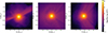 |
Fig. 1. Planar slices of runaway-star density 1000 seconds after explosion. A slight asymmetry and a non-spherical extension of the ejecta are visible outside the inner 0.05 R⊙. |
3. Mapping the hydrodynamical result in the 1D stellar evolution code MESA
To model the long-term evolution of the remnant runaway, we evolved it in MESA. The components of the MESA EOS blend relevant to this work are FreeEOS (Irwin 2004), near the surface of the models, and HELM (Timmes & Swesty 2000) and Skye (Jermyn et al. 2021), for white dwarf cores. MESA uses tabulated radiative opacities primarily from OPAL (Iglesias & Rogers 1993, 1996), with low-temperature data from Ferguson et al. (2005) and the high-temperature, Compton-scattering-dominated regime by Poutanen (2017). The electron conduction opacities are from Cassisi et al. (2007). Nuclear reactions are from JINA REACLIB (Cyburt et al. 2010), NACRE (Angulo et al. 1999), and additional tabulated weak reaction rates (Fuller et al. 1985; Oda et al. 1994; Langanke & Martínez-Pinedo 2000). The screening of reaction rates was included according to the prescription of Chugunov et al. (2007), while thermal neutrino-loss rates are from Itoh et al. (1996). The initial white dwarf models were made with the make_co_wd test suite, with the solar composition of Asplund et al. (2009). The white dwarf masses are then relaxed to the masses of our models using the relax_mass hook (see Table 1).
Runaway composition as function of total mass.
In previous work by Bhat et al. (2025), the change in thermal state of the post-explosion runaway white dwarf donor compared to the pre-explosion donor was used to map the change in entropy that the donor star experiences as a result of interaction with the supernova ejecta. In this study, the final runaway star configuration was not only a result of supernova stripping and shock heating (as was the case in Bhat et al. 2025), it was also affected by the disruption of the secondary white dwarf just before the explosion (as was the case in Glanz et al. 2025). That is, we believe the thermal state of this runaway is also dominated by the hydrodynamics just before the supernova, which are captured in the Arepo model. They are less sensitive to the thermal state of the model prior to interaction with its companion, and we can therefore map the Arepo entropy more directly into MESA, rather than relying on an entropy difference. Furthermore, defining an entropy difference is more complicated for this system since the donor loses more than 75% of its mass. Since MESA is a 1D evolutionary code, we averaged the 3D profiles from AREPO. We employed the averaged profiles directly by repurposing the MESA relaxation test suite relax_composition_j_entropy to initialise a WD model directly to the entropy and composition profile specified by the final state of the AREPO model. Here, the procedure followed is similar to that outlined in Glanz et al. (2025). Since the overall mass loss is too high and the WD is almost completely disrupted, we did not use the heating approach used in Bhat et al. (2025) to generalise the heating for multiple white dwarfs. For this work, we did not use any external opacity tables and relied on the Type II opacities in MESA. We neglect diffusion for now. Since these stars are cooler and have lower surface gravities compared to the new hypervelocity stars discovered by El-Badry et al. (2023), we do not expect diffusion to play a big role for the time that we evolve them.
Since the boundary of the post-explosion runaway is difficult to average (due to the non-spherical nature of the bound object, as shown in Figure 4), we averaged on equipotential surfaces of the gravitational potential. This is different than the spherical averaging employed before by Bhat et al. (2025) and Glanz et al. (2025), and it is preferred because our system is non-spherical. Furthermore, we define four models with different cuts to the outer parts of the profile by the approximate energy regimes, as shown in Figure 4. The first cut is defined by the decay energy of 56Ni being more than twice the gravitational energy. This is 0.154 M⊙. The second cut is defined by the limit that the Arepo model is spherically symmetric, such that the specific radial energy, defined as vr2/2, where vr is the averaged velocity in the radial direction, is less than 1%. This model has a mass of 0.12 M⊙. The third cut is chosen in between the first two masses around 0.14 M⊙, where the gravitational energy dominates but the kinetic and decay energies are still significant. The final cut is a lower limit at 0.10 M⊙. This model has no significant (> 10−5 in mass fraction) supernova pollution. These mass cuts allowed us to evolve multiple stars with different amounts of elements at the surface. Since we skipped the dynamical evolution of the remnant before it reaches full spherical hydrostatic equilibrium due to computational limitations, spherical averaging is only approximate in the outer regions of the remnant. We can therefore capture some uncertainty that is associated with the 3D averaging by making these mass cuts.
From the theory of tides, one would expect the donor white dwarf to rotate extremely fast (∼40 seconds) to come close to the orbital period (Marsh et al. 2004; Fuller & Lai 2012, 2014; Yu et al. 2020). However, due to the tidal distortion pre-supernova and the total disruption by the supernova with the corresponding expansion of the surviving star, the post-supernova runaway shows almost negligible rotation. From Figure 2, assuming angular momentum of ∼1048 g cm2 s−1 and a mass of 0.15 M⊙, the period of rotation for a radius of 0.1 R⊙ is about 10.5 hours. This increases, however, to ∼10 days for a radius of 0.5 R⊙; it is closer to the observed radius for these stars (assuming rigid body rotation). As the star would contract over time, this rotation rate should increase, but it will only become significant once the star is on its cooling track. Much of the angular momentum of the system is lost in the disruption, and all but the very core of the donor white dwarf is stripped. We therefore did not consider any rotation in our models. D6-2 rotates with a period of 15.4 hours (Chandra et al. 2022), but it most likely does not come from this scenario; the other runaways are not yet known to harbour significant rotation. J1637 was confirmed to have an upper limit of 40 km s−1 by Hollands et al. (2025) based on the spectral resolution and stellar-line broadening.
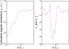 |
Fig. 2. Total angular momentum and rotational velocity of the runaway at around 1000 s after the explosion. The plotted quantities are spherical averages and highlight the differences in the state of the stellar interior. Most of the angular momentum is within 0.1 R⊙. While the external (> 0.1 R⊙) has some residual rotation and radial energy this is only in a small region that forms a stream-like structure. |
For all evolution and relaxation scenarios, we used the approx21_plus_co56 nuclear network. This includes the isotopes 1H, 3, 4He, 12C, 14N, 16O, 20Ne, 24Mg, 28Si, 32S, 36Ar, 40Ca, 44Ti, 48, 56Cr, 52, 54, 56Fe, 56Co, and 56Ni.
4. Long-term evolution
As described in Bhat et al. (2025) and Glanz et al. (2025), we carried out the subsequent evolution after relaxation to a maximum age of 100 Myr. We enabled nuclear burning, convection, and thermohaline mixing (Kippenhahn et al. 1980). Compared to the WDs produced by the D6 scenario in previous works (Pakmor et al. 2022), there is much less radioactive material here. Nevertheless, the atmosphere is still slightly polluted. We also switched on super-Eddington winds for mass loss driven by any 56Ni decay, but found that at no time is this energy enough to unbind any surface layers.
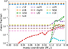 |
Fig. 3. Main elements as function of mass coordinate for runaway 1000 s after the supernova for mass coordinates that remain bound after supernova explosion. Unlike in Bhat et al. (2025), 56Ni does not dominate the mass fraction at the surface of the runaway. 56Fe is present due to the primordial solar abundance assumed. 20Ne and 24Mg are elevated most likely due to carbon burning on the secondary. |
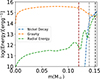 |
Fig. 4. Different energies in runaway WD as function of its mass coordinate. The black line marks the region where nickel decay dominates, the grey line marks the region where gravity dominates over other energies, and the brown line marks the region where gravity is the only relevant energy. Rotational energy is not shown as it is negligible. Radial energy is defined as vr2/2. |
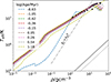 |
Fig. 5. Structural profile of 0.154 M⊙ model as a function of its age. The puffing up and later contraction of the star are seen here. The black circles (black squares) represent 50% (90%) of the stellar mass. The dashed-dotted grey line is the degeneracy limit above which gas pressure dominates. The two grey lines in the bottom right are the crystallisation limit for carbon and oxygen. Dotted regions are convective. |
The evolution of the 0.154 M⊙ model is slightly similar to what was seen for the D6 runaways in Bhat et al. (2025), but in a completely different phase space of the HR-diagram. In particular, our models are close to the boundary of degeneracy, even in the stellar core. For this reason, we do not consider the runaway stars to be white dwarfs at this particular stage of their evolution. The evolution of the ρ − T profile is shown in Figure 5 for this model. As the star was almost completely disrupted, its density is significantly lower than that of the pre-supernova donor. As such, for the early stages of the evolution, almost 50% of the stellar mass is close to the degeneracy limit given by the Fermi energy being equal to the thermal energy, EF = kBT. The outer 10% of the star by mass is non-degenerate. Over the first 105 yr this region of the star expands, while the inner region contracts and becomes hotter. The entirety of the star becomes close to completely degenerate by the time ∼10 Myr has passed. Our models only come close to their corresponding cooling track at the end of our simulations (at 100 Myr). This rho-T space shows the evolution to a configuration similar to the lowest mass models in Shen (2025) for the external 10% of the star. The total initial configuration is different, however, since the models of Shen (2025) are purely convective, have no degenerate material, and are significantly cooler.
While this model does not have significant 56Ni, some decay still occurs and produces iron. For 7 × 10⁻⁵ M⊙ of 56Ni, this amounts to around 1046 erg. Within our models, the highest specific luminosity is ∼108 erg/g/s at the beginning of the evolution. This is enough to heat the runaway star significantly to expand, but, as this drops exponentially, the heating is not sustained long enough to lose any mass due to the Eddington luminosity limit. For our models, this limit is close to  . Such a luminosity is only produced in the first few days of the nickel decay and is not sustained long enough for the star to reach super-Eddington luminosity at the surface. Much of this energy is channelled into the expansion of the star as it thermally re-adjusts. Furthermore, this expansion in the first year following the supernova is sensitive to our choice of the surface cut. Due to issues with numerical convergence, we were not able to evolve the model with the complete amount of 56Ni it captured. It is possible that the total amount is sufficient to launch a wind. This could explain the CaII emission-line velocity of ∼200 km s−1 from a surviving companion reported by Siebert et al. (2023), which is close to the escape velocity:
  km s−1 for 0.154 M⊙ and radius 0.5 R⊙.
Since the MESA thermohaline mixing procedure does not model the impact of the heavier metals in the surface layers where FreeEOS tables are used, we also applied minimal mixing in the outer ∼3% of the mass of the star, similarly to what was done in Bhat et al. (2025). For all the other models where no significant amount of supernova contamination exists due to surface cuts, the evolution of the runaway star is very similar to this model after 1000 yr (that is, after the nickel has decayed). For those models, the nuclear-decay energy is only of the order of 102 − 104 erg/g/s for the first ∼100 days and decays exponentially. The evolution of these models is dominated by thermal adjustment due to tidal heating near disruption and the heat injected by the supernova shock, until the subsequent contraction and cooling towards the white dwarf cooling track.
5. Comparison with observations
The Hertzsprung-Russell (HR) and Kiel diagrams of all the models are shown in Figure 6, with the hypervelocity stars over-plotted. For a discussion on the values of radius, surface temperature, and surface gravity of all except one object (J1637), we refer the reader to Bhat et al. (2025). We omitted the hottest star, J0546, because it is far outside the parameter range of our models; we instead plot the new star J1637 (Hollands et al. 2025), which fits better here. For J1332, we considered the hydrogen-dominated model from Werner et al. (2024). Although the presence of this hydrogen should not be automatically assumed (El-Badry et al. 2023; Glanz et al. 2025), it may be explained by Bondi-Hoyle-Lyttleton accretion of ∼ 10−16 M⊙ hydrogen from the ISM (Werner et al. 2024; Shen 2025). The luminosity was calculated using
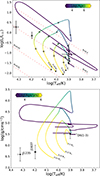 |
Fig. 6. Upper panel: HR diagram for all surface cuts. All observed hypervelocity stars are plotted as black points. Dashed red lines represent lines of constant radii. The colour bar shows the log(age) of the star. Markers show the ages at 104, 105, 106, 107, 108 years. Lower panel: The Kiel diagram for the same model. |
 (2)
(2)
Unlike the models of Bhat et al. (2025), the models here do not have significant radioactive nickel, due to which the stars cool in the beginning with a roughly constant radius. This process is disrupted by the internally deposited heat of the star (and in the case of one model, the nickel decay) making its way to the surface as the runaway star starts to expand and increase its luminosity. The evolutionary tracks of our lower mass models pass through the positions of D6-1 and D6-3, showing for the first time that survivors of violent mergers might be able to explain these stars.
5.1. Radius and Teff
A more precise comparison with the observed values is needed to gauge whether the expansion occurs on a timescale similar to that of the observational timescale of these stars. The evolution of radius, effective temperature, and surface gravity of our models over time is shown in Figure 7. The models puff up at approximately 104 yr for the highest mass model to 106 yr for the lowest mass model. This is seen in the radius and surface gravity plots. The increase in surface temperature corresponds to the contraction after the star has puffed up to its maximum radius. We also over-plot the relevant hypervelocity stars again with their kinematic ages taken from Bhat et al. (2025).
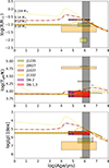 |
Fig. 7. Evolution of radius, effective temperature, and surface gravity of our models. Observed hypervelocity stars are plotted here for the radius. While the radii of D6-1 and D6-3 are similar to those of D6-2, their age estimate is less certain and spans a bigger region. Due to the association of D6-2 with the supernova remnant (SNR) G70.0–21.5, the purple box is the truncated age estimate for D6-2. The grey band is the mid-plane crossing time for D6-1 and D6-3 taken from Bhat et al. (2025), which assumed they were ejected from the disc and is therefore less wide than the red bands. |
To understand the relation of the kinematic age and the expansion of the star, we can look at the relevant timescales. The expansion and heating of the stars is governed by two thermal timescales. The local thermal timescale, according to Zhang et al. (2019), is given as
 (3)
(3)
where H = P/ρg is the local pressure scale height, and Dth = 4acT3/3κρ2cP is the coefficient of thermal diffusion. This timescale is relevant for the local heat transfer within any star and sets the time for the runaway star to transfer the internal heat to the surface, allowing the star to readjust. In comparison, the Kelvin-Helmholtz timescale sets the timescale of runaway-star cooling once this heat has been fully transferred outside. This is given by
 (4)
(4)
The upper panel of Figure 8 shows the initial thermal timescales of the models. The sudden increase of the local thermal timescale in the outer layers is due to the surface contamination. The local pressure scale height and the opacity change the timescale associated with those layers. The middle panel shows an example of the 0.12 M⊙ model with an approximate estimate of local heating as a fraction of the internal energy e, TΔS/e plotted alongside the thermal timescale. Unlike what was the case in Bhat et al. (2025), where the massive white dwarfs were only heated in layers with timescales of a few thousand years, the surface heating here is significant, and the local thermal timescale approximately corresponds to the kinematic ages of the observed runaways. A similar result was found for lower mass stars by Zhang et al. (2019), although they did not start with a 3D simulation. The evolution of the Kelvin-Helmholtz time is shown in the lowest panel. This timescale is lower for the higher mass models, which have a higher luminosity in the beginning. Once all the models have reached thermal equilibrium, this time is of the same order as that at the beginning of the cooling track. This figure therefore shows that for these models the observed kinematic ages match the thermal timescales and can help explain why these stars are slightly inflated over the observed times.
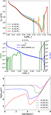 |
Fig. 8. Upper panel: Local thermal timescale as function of mass coordinate for the four models. Middle panel: Heating fraction (green) and thermal timescale (blue) for the 0.12 M⊙ model. Lower panel: Kelvin-Helmholtz timescale of the models as a function of age. |
5.2. Surface abundances
Our lower mass models < 0.15 M⊙ have allowed us to study the heating and expansion of the runaway star due to the supernova shock and stripping in detail. However, the surface abundances of D6-1 and D6-3 show significant Ne, Mg, and Ca, apart from C and O, and cannot be explained by those models. The 0.154 M⊙ model allows these elements to be studied directly. In Figure 9, we show how the surface abundances evolve for our models.
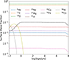 |
Fig. 9. Mass fraction of elements that contribute significantly to the surface composition of the 0.154 M⊙ model. The drop of these fractions in the later ages is due to thermohaline mixing. |
Within the temperature range of our models, iron opacities are of the order of 0.01 − 0.1 cm2/g, and one needs a luminosity close to or higher than the Eddington luminosity for radiative levitation. This is different than the case of the hotter WDs from Bhat et al. (2025) that were hotter than 105 K, where the iron opacity bump decreases this luminosity to 102 − 103 L⊙. Therefore, for our models, thermohaline mixing and convection are the main sources of heat transfer and mixing throughout the star.
5.3. Observations of supernova remnants
One of the key puzzles in the observations of hypervelocity stars from thermonuclear explosions is the lack of any runaways around known Type Ia SNRs (Kerzendorf et al. 2013, 2014, 2018; Shields et al. 2022, 2023). One of the plausible solutions is that most Type Ia supernovae that occur in white dwarf binaries are quadruple detonations. In such a case, the donor white dwarf also explodes due to the compression from the supernova shock igniting helium (Shen et al. 2024; Boos et al. 2024). However, if the violent merger scenario contributes 1 − 2% to this population, then a runaway must exist in 1 − 2% of SNRs.
A second possibility is that a potential runaway was missed because all models have so far predicted stars bigger than a solar radius and/or with surface temperatures greater than 10 000 K. Our model, on the contrary, shows that for the time when the runaway should still be inside the remnant (∼1000 yr), it is actually under-luminous and cool compared to what was shown by other models. Our model-stars are less than one solar radius and < 10 000 K in surface temperature, leading to an average luminosity that is less than solar. In comparison, the models of Bhat et al. (2025) and Glanz et al. (2025) are over-luminous by four orders of magnitude and hot enough to have significant UV emission. While optical and infrared observations might be helpful in the future, these observations could be contaminated by the SNR itself.
We recreated Figure 5 of Shields et al. (2023), which compared the stars within the SNR 0509−67.5 in the LMC with models of Type Ia-surviving donors. The control stars represent the main sequence outside of the central region, while the centre stars were considered as possible runaways since they are close to the centre of the SNR. The models of Bhat et al. (2025) and Glanz et al. (2025) that came after this study would also have been discarded as they were hotter and inflated. The recent models of Wong & Bildsten (2025) could be considered as long as the HeWD is less than 0.3 M⊙. Our new model cannot be discarded right now, as shown in Figure 10, and it therefore provides a new avenue to study this and similar regions again. It was recently shown by Das et al. (2025) that SNR 0509−67.5 was most likely a sub-Chandrasekhar detonation. Their evidence for double shell morphology hints at a double or quadruple detonation, which is also consistent with Prust et al. (2026). A study of the parameter space mentioned here will, however, be another test to confirm this. For the case of SN 1006, where no hypervelocity star was found by Shields et al. (2022), it is possible that no remnant survived, since all proper-motion outliers are in the main sequence, unless the star was ejected in our direction. If a runaway exists, our models suggest that the star would have to be < 0.1 M⊙ to be faint enough not to be found in the extended search regime.
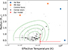 |
Fig. 10. LMC SNR sample from Shields et al. (2023). Overlaid is the radius and effective temperature taking into account all four of our models in red and the other He- and main-sequence-star models (MS) that were discarded by Shields et al. (2023). |
6. The formation of hypervelocity stars from white dwarf binaries
We show that the violent merger scenario is a possible way of producing cooler CO-dominated hypervelocity stars. For the hotter ones, merger-disruptions in HeCO WDs (Glanz et al. 2025) and double detonations through Roche-lobe-filling white dwarf donors (Pakmor et al. 2022) have previously been studied. In Figure 11, all of the known tracks from these three models are plotted to create a unifying picture of the fate of the donor white dwarf in white dwarf binaries. To bridge the gap, we added one track of 0.3 M⊙ taken from the recent work of Shen (2025). Despite not originating from a 3D explosion simulation, the model can be used to estimate the heating of heavier mass remnants from our merger scenario. For the purpose of clarity, we only plot the tracks after the first 1000 years of evolution, which are mainly dominated by super-Eddington expansion for the more massive white dwarfs.
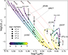 |
Fig. 11. HR diagram for all models. All observed hypervelocity stars are plotted as black points. Dashed red lines represent lines of constant radii. The colour bar shows the log(age) of the star. The middle model going through J1235 is the 0.3 M⊙ model from Shen (2025), plotted with a dotted line to differentiate it from the other models for which a 3D simulation exists. |
The main difference between our work and the models of Shen (2025) is that our 3D model shows that these stars are not completely convective and are partially degenerate. Figure 12 compares the specific entropy of our 0.154 M⊙ model with a 0.154 M⊙ fully convective star similar to those in Shen (2025), but calculated with MESA version 24.08.1 and the Type 2 opacities included with MESA (for a better comparison to the models presented in this work) at three different luminosities. Their models show a near constant inner entropy profile with changes occurring near the surface. Our models have a comparatively lower entropy near the centre, but a higher entropy close to the surface. As such, the local thermal time and not the Kelvin-Helmholtz time determine the inflated radii of the observed stars.
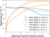 |
Fig. 12. Specific entropy as function of fractional mass below surface for our 0.154 M⊙ model and the 0.154 M⊙ fully convective model similar to the work of Shen (2025). Three surface luminosities are plotted for comparison. |
In terms of the values presented here and assuming that J1332 is a hypervelocity star, J1332 may be explained by the double detonation scenario. No other hypervelocity runaway matches our models from the double-detonation scenario, unless the donors somehow lose more mass and become less massive than 0.5 M⊙ in the supernova that follows. This is highly unlikely, as the simulation of the 0.7 M⊙ white dwarf has previously shown. While the 0.5 M⊙ white dwarf has lower internal pressure, it would be farther away from the accretor, and therefore the shock would not necessarily strip away even more material. Beyond this limit, HeWD donors to massive CO WDs accretors may be able to explain the radius and temperature, but they fail to explain the high speeds of the stars. HeWDs can only reach up to ∼1600 km s−1 (Wong & Bildsten 2025).
The merger-disruption method of Glanz et al. (2025) offers a way to create the hotter runaways with increased speeds that stay expanded for long enough. Including our study, it is likely that these stars represent the runaway distribution from the lower mass end of the initial white dwarfs, whereas CO WD progenitors, as studied here, could represent the higher mass end. Depending on the mass ratio and the amount of helium in the system, mass loss could be significant in bridging the gap between 0.15 and 0.48 M⊙. The new runaway J1637 and J1235 are both examples of systems that might have formed in such mergers. While not matching the kinematic ages exactly, the recent models of Shen (2025) show that is indeed possible.
For the case of merging white dwarfs, the Roche-lobe approximation for orbital velocities used by Bauer et al. (2021) and El-Badry et al. (2023) underestimates their final velocities. This is because those calculations assume a supernova detonation when the donor WD has only just begun to overflow its Roche lobe. In contrast, merging WDs evolve significantly beyond this point, reaching closer to their companions and boosting their velocities further before detonation occurs. A better analytical velocity estimate can therefore be given by the circularisation radius of the disrupted secondary (subscript 2 in the following). Upon Roche-lobe overflow, the separation is given by aRoche. Under the assumption that the angular momentum at this point, dominated by the binary motion, is conserved, the circularisation radius of the disrupted white dwarf is given by (see Eq. (1) of Fernández & Metzger 2013)
 (5)
(5)
Based on this radius, we can calculate an upper bound of the orbital velocity for the donor at the point of explosion as a function of the orbital velocity when the secondary first fills the Roche lobe given in Bauer et al. (2021):
 (6)
(6)
Here, vRoche is defined as the orbital velocity at aRoche of the secondary, given as  . Following Eggleton (1983), we obtain Equation (2) of Bauer et al. (2021):
  . However, a major assumption in the derivation above is that the secondary is completely disrupted to form a torus around the primary. This is obviously not the case in reality, since an explosion happens before such a state can be reached. Therefore, the centre of mass (COM) of the system is still not at the centre of the primary, but close to it. A simple analytical expression to calculate the ejection velocity as the orbital velocity with respect to the COM is therefore given by assuming that the distance of the secondary to the COM is approximately rcirc/(1 + q), leading to
 (7)
(7)
This is equivalent to
![Mathematical equation: $$ \begin{aligned} v_{\rm circ} = \sqrt{\frac{0.49\,q^{2/3}\;GM_1}{R_2 \left[0.6\,q^{2/3} + \ln (1+q^{1/3})\right]}}\cdot \end{aligned} $$](/articles/aa/full_html/2026/02/aa57683-25/aa57683-25-eq12.gif) (8)
(8)
This velocity is plotted in Figure 13 in a similar manner to that in Glanz et al. (2025), although the assumption was that there was tidal disruption and the mass range was relatively smaller. The figure clearly shows that the orbital velocities allowed for merging white dwarfs can be much higher than previously assumed. The slight excess velocity in the simulation is most likely due to the final surviving part of the white dwarf being even closer than this radius as well as the angular-momentum loss, which will result in an even closer object, but is neglected in the analytical calculation. Since the calculation only works for the COM, part of the donor would plunge in faster than this velocity. Furthermore, a kick velocity of ∼400 km s−1 was seen in the simulation that would bring the ejection velocity closer to the calculated orbital velocity by 100 km s−1.
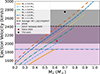 |
Fig. 13. Orbital velocities for multiple primary and secondary masses (the lines correspond to different primaries). The velocity is calculated assuming the circularisation radius is reached before explosion. Two simulation values are plotted as circles. The black region shows min and max ejection velocities for D6-1,3, J1235, and J0927. Cyan and purple lines (and the corresponding shaded regions) show the values for J1637 and J0546, respectively, both matching slightly lower mass white dwarf secondaries. |
The calculation to explain the significant mass loss is not as straightforward but can be motivated by previous studies (Bauer et al. 2019; Wong & Bildsten 2025). The ejecta from the supernova hit the donor (M2) with a ram pressure equal to
 (9)
(9)
Since a (close to disruption) scales inversely with donor mass, massive donors with massive accretors will experience higher ejecta ram pressure. At the separation we calculated above, the ejecta pressure would be (1 + q)3 times more than the pressure when they start to fill their Roche lobes (as was the case for the D6 scenario in Pakmor et al. 2022). A second important quantity is the pressure within the donor, which may be characterised by the central pressure, which scales with M22/R24. A consequence of this is that despite feeling a higher pressure, the corresponding shock strength is lower in more massive CO white dwarfs compared to hot subdwarfs and He white dwarfs (Bauer et al. 2019; Wong & Bildsten 2025). This leads to a lower fraction of mass loss and shock heating in more massive white dwarfs (Bhat et al. 2025). However, white dwarfs close to disruption have significant rotational energy and are tidally heated and significantly distorted. Due to the dynamically unstable nature of mass transfer in white dwarfs, the secondary will also be puffier due to mass loss before the explosion. This can change the central pressure and deviate significantly from the simple polytropic consideration. The inverse dependence of the pressure on R4 also causes this pressure to drop very quickly. This is also clear from Figure 5, where even after a few thousand seconds the runaway star is only partially degenerate. Furthermore, our simulation shows that the centre of the secondary goes from > 108 g/cm3 at the beginning of the simulation to ∼107 g/cm3 before the explosion. A similar drop in central pressure is seen, such that the ejecta pressure is of the same order as the central pressure. If the outer layers of the white dwarfs are close to complete disruption, the mass loss will be set by the ram pressure due to the incoming ejecta, the coupling of this ejecta with the secondary, and how disrupted the secondary white dwarf is at that moment. Therefore, as the donor and accretor masses increase, the donor could in some cases lose significantly more of its mass, and therefore lower mass runaways could be expected to form. This is probably why our system ends up with a lower mass runaway than the one in Glanz et al. (2025). Furthermore, exactly how much mass is lost before the detonation of the primary and how much is lost after is not completely clear due to the complex dynamics involved. Future simulations should help shed more light on these questions.
This work shows the difference that helium-shell masses can make in the final fates of white dwarf binaries. Pakmor et al. (2022) started with a 0.7 + 1.05 M⊙ system. Here, we started with 0.7 + 1.1 M⊙. Despite almost identical mass ratios, the final results are drastically different. If the helium-shell mass on the primary is much lower (0.0003 M⊙ as used here and as calculated by Shen et al. 2024) initially, the double detonation mechanism can be avoided. Then, the mass transfer can proceed until the primary explodes due to carbon ignition and the secondary is significantly disrupted.
7. Conclusions
In this paper, we present results of a 3D simulation and corresponding 1D stellar evolution of a runaway star produced from the violent merger supernova scenario for the first time. In the cases when the primary white dwarf does not undergo double detonation to create a supernova, the secondary white dwarf can continue mass transfer and come closer to the primary. On its last orbit, close to the circularization radius of the system, the secondary is almost completely distorted, and the resulting infall ignites carbon on the primary white dwarf and destroys it. In the aftermath, a relatively low-mass (0.16 M⊙) chunk of the donor flies away at a speed roughly ( ) times the orbital velocity at the beginning of Roche-lobe overflow.
We mapped the simulation results in MESA to evolve heated white dwarfs representing surviving chunks of pre-supernova donors in the mass range of 0.10 M⊙ − 0.156 M⊙. We then evolved these models to 100 Myr after the supernova explosion. Our results match the observed values of the cooler stars quite well. In particular, the thermal times of these models match the kinematic ages of the observed hypervelocity stars. With future studies, the parameter range of the violent merger scenario and the resulting runaway masses must be explored.
Our study reopens the possibility to revisit observations of supernova remnants for hypervelocity elopers. Since these stars are not as hot and contaminated as previously believed, they might be hiding in the surrounding main-sequence population.
Acknowledgments
This project succeeded a project which was originally started as part of the Kavli Summer Program which took place in the Max Planck Institute for Astrophysics in Garching in July 2023, supported by the Kavli Foundation. AB is extremely grateful to Stephen Justham and Selma de Mink for not listening to him back then, and assigning him the runaway project. We would also like to thank the anonymous referee for their helpful report and comments. A.B. was supported by the Deutsche Forschungsgemeinschaft (DFG) through grant GE2506/18-1. K.J.S. was supported by NASA through the Astrophysics Theory Program (80NSSC20K0544) and by NASA/ESA Hubble Space Telescope programs #15871 and #15918. Work by EB was performed under the auspices of the U.S. Department of Energy by Lawrence Livermore National Laboratory under Contract DE-AC52-07NA27344.
References
- Angulo, C., Arnould, M., Rayet, M., et al. 1999, Nucl. Phys. A, 656, 3 [Google Scholar]
- Asplund, M., Grevesse, N., Sauval, A. J., & Scott, P. 2009, ARA&A, 47, 481 [NASA ADS] [CrossRef] [Google Scholar]
- Bauer, E. B., White, C. J., & Bildsten, L. 2019, ApJ, 887, 68 [Google Scholar]
- Bauer, E. B., Chandra, V., Shen, K. J., & Hermes, J. J. 2021, ApJ, 923, L34 [NASA ADS] [CrossRef] [Google Scholar]
- Bhat, A., Bauer, E. B., Pakmor, R., et al. 2025, A&A, 693, A114 [NASA ADS] [CrossRef] [EDP Sciences] [Google Scholar]
- Bondi, H. 1952, MNRAS, 112, 195 [Google Scholar]
- Boos, S. J., Townsley, D. M., Shen, K. J., Caldwell, S., & Miles, B. J. 2021, ApJ, 919, 126 [NASA ADS] [CrossRef] [Google Scholar]
- Boos, S. J., Townsley, D. M., & Shen, K. J. 2024, ApJ, 972, 200 [NASA ADS] [CrossRef] [Google Scholar]
- Cassisi, S., Potekhin, A. Y., Pietrinferni, A., Catelan, M., & Salaris, M. 2007, ApJ, 661, 1094 [NASA ADS] [CrossRef] [Google Scholar]
- Chandra, V., Hwang, H.-C., Zakamska, N. L., et al. 2022, MNRAS, 512, 6122 [CrossRef] [Google Scholar]
- Chugunov, A. I., Dewitt, H. E., & Yakovlev, D. G. 2007, Phys. Rev. D, 76, 025028 [NASA ADS] [CrossRef] [Google Scholar]
- Cyburt, R. H., Amthor, A. M., Ferguson, R., et al. 2010, ApJS, 189, 240 [NASA ADS] [CrossRef] [Google Scholar]
- Dan, M., Rosswog, S., Guillochon, J., & Ramirez-Ruiz, E. 2011, ApJ, 737, 89 [NASA ADS] [CrossRef] [Google Scholar]
- Dan, M., Rosswog, S., Guillochon, J., & Ramirez-Ruiz, E. 2012, MNRAS, 422, 2417 [NASA ADS] [CrossRef] [Google Scholar]
- Das, P., Seitenzahl, I. R., Ruiter, A. J., et al. 2025, Nat. Astron., 9, 1356 [Google Scholar]
- Eggleton, P. P. 1983, ApJ, 268, 368 [Google Scholar]
- El-Badry, K., Shen, K. J., Chandra, V., et al. 2023, Open J. Astrophys., 6, 28 [CrossRef] [Google Scholar]
- Ferguson, J. W., Alexander, D. R., Allard, F., et al. 2005, ApJ, 623, 585 [Google Scholar]
- Fernández, R., & Metzger, B. D. 2013, ApJ, 763, 108 [CrossRef] [Google Scholar]
- Fink, M., Hillebrandt, W., & Röpke, F. K. 2007, A&A, 476, 1133 [NASA ADS] [CrossRef] [EDP Sciences] [Google Scholar]
- Fuller, J., & Lai, D. 2012, MNRAS, 421, 426 [NASA ADS] [Google Scholar]
- Fuller, J., & Lai, D. 2014, MNRAS, 444, 3488 [NASA ADS] [CrossRef] [Google Scholar]
- Fuller, G. M., Fowler, W. A., & Newman, M. J. 1985, ApJ, 293, 1 [NASA ADS] [CrossRef] [Google Scholar]
- Glanz, H., Perets, H. B., Bhat, A., & Pakmor, R. 2025, Nat. Astron., 9, 1523 [Google Scholar]
- Guillochon, J., Dan, M., Ramirez-Ruiz, E., & Rosswog, S. 2010, ApJ, 709, L64 [Google Scholar]
- Hollands, M. A., Shen, K. J., Raddi, R., et al. 2025, MNRAS, 541, 2231 [Google Scholar]
- Hoyle, F., & Lyttleton, R. A. 1939, Proc. Camb. Philos. Soc., 35, 405 [CrossRef] [Google Scholar]
- Iglesias, C. A., & Rogers, F. J. 1993, ApJ, 412, 752 [Google Scholar]
- Iglesias, C. A., & Rogers, F. J. 1996, ApJ, 464, 943 [NASA ADS] [CrossRef] [Google Scholar]
- Irwin, A. W. 2004, Astrophysics Source Code Library [record ascl:1211.002] [Google Scholar]
- Itoh, N., Hayashi, H., Nishikawa, A., & Kohyama, Y. 1996, ApJS, 102, 411 [NASA ADS] [CrossRef] [Google Scholar]
- Jermyn, A. S., Schwab, J., Bauer, E., Timmes, F. X., & Potekhin, A. Y. 2021, ApJ, 913, 72 [NASA ADS] [CrossRef] [Google Scholar]
- Jermyn, A. S., Bauer, E. B., Schwab, J., et al. 2023, ApJS, 265, 15 [NASA ADS] [CrossRef] [Google Scholar]
- Kerzendorf, W. E., Yong, D., Schmidt, B. P., et al. 2013, ApJ, 774, 99 [NASA ADS] [CrossRef] [Google Scholar]
- Kerzendorf, W. E., Childress, M., Scharwächter, J., Do, T., & Schmidt, B. P. 2014, ApJ, 782, 27 [NASA ADS] [CrossRef] [Google Scholar]
- Kerzendorf, W. E., Strampelli, G., Shen, K. J., et al. 2018, MNRAS, 479, 192 [NASA ADS] [CrossRef] [Google Scholar]
- Kippenhahn, R., Ruschenplatt, G., & Thomas, H. C. 1980, A&A, 91, 175 [Google Scholar]
- Kromer, M., Sim, S. A., Fink, M., et al. 2010, ApJ, 719, 1067 [Google Scholar]
- Langanke, K., & Martínez-Pinedo, G. 2000, Nucl. Phys. A, 673, 481 [NASA ADS] [CrossRef] [Google Scholar]
- Marsh, T. R., Nelemans, G., & Steeghs, D. 2004, MNRAS, 350, 113 [NASA ADS] [CrossRef] [Google Scholar]
- Moll, R., & Woosley, S. E. 2013, ApJ, 774, 137 [NASA ADS] [CrossRef] [Google Scholar]
- Oda, T., Hino, M., Muto, K., Takahara, M., & Sato, K. 1994, At. Data Nucl. Data Tab., 56, 231 [NASA ADS] [CrossRef] [Google Scholar]
- Pakmor, R., Kromer, M., Röpke, F. K., et al. 2010, Nature, 463, 61 [Google Scholar]
- Pakmor, R., Kromer, M., Taubenberger, S., et al. 2012, ApJ, 747, L10 [NASA ADS] [CrossRef] [Google Scholar]
- Pakmor, R., Kromer, M., Taubenberger, S., & Springel, V. 2013, ApJ, 770, L8 [Google Scholar]
- Pakmor, R., Springel, V., Bauer, A., et al. 2016, MNRAS, 455, 1134 [Google Scholar]
- Pakmor, R., Callan, F. P., Collins, C. E., et al. 2022, MNRAS, 517, 5260 [NASA ADS] [CrossRef] [Google Scholar]
- Pakmor, R., Shen, K. J., Bhat, A., et al. 2025, ArXiv e-prints [arXiv:2510.11781] [Google Scholar]
- Paxton, B., Bildsten, L., Dotter, A., et al. 2011, ApJS, 192, 3 [Google Scholar]
- Paxton, B., Cantiello, M., Arras, P., et al. 2013, ApJS, 208, 4 [Google Scholar]
- Paxton, B., Marchant, P., Schwab, J., et al. 2015, ApJS, 220, 15 [Google Scholar]
- Paxton, B., Schwab, J., Bauer, E. B., et al. 2018, ApJS, 234, 34 [NASA ADS] [CrossRef] [Google Scholar]
- Paxton, B., Smolec, R., Schwab, J., et al. 2019, ApJS, 243, 10 [Google Scholar]
- Poutanen, J. 2017, ApJ, 835, 119 [NASA ADS] [CrossRef] [Google Scholar]
- Prust, L. J., Bildsten, L., & Boos, S. J. 2026, ApJ, 997, 17 [Google Scholar]
- Sato, Y., Nakasato, N., Tanikawa, A., et al. 2015, ApJ, 807, 105 [NASA ADS] [CrossRef] [Google Scholar]
- Shen, K. J. 2025, ApJ, 982, 6 [Google Scholar]
- Shen, K. J., Boubert, D., Gänsicke, B. T., et al. 2018a, ApJ, 865, 15 [Google Scholar]
- Shen, K. J., Kasen, D., Miles, B. J., & Townsley, D. M. 2018b, ApJ, 854, 52 [Google Scholar]
- Shen, K. J., Boos, S. J., & Townsley, D. M. 2024, ApJ, 975, 127 [NASA ADS] [CrossRef] [Google Scholar]
- Shields, J. V., Kerzendorf, W., Hosek, M. W., et al. 2022, ApJ, 933, L31 [NASA ADS] [CrossRef] [Google Scholar]
- Shields, J. V., Arunachalam, P., Kerzendorf, W., et al. 2023, ApJ, 950, L10 [NASA ADS] [CrossRef] [Google Scholar]
- Siebert, M. R., Foley, R. J., Zenati, Y., et al. 2023, ApJ, 958, 173 [NASA ADS] [CrossRef] [Google Scholar]
- Springel, V. 2010, MNRAS, 401, 791 [Google Scholar]
- Timmes, F. X., & Swesty, F. D. 2000, ApJS, 126, 501 [NASA ADS] [CrossRef] [Google Scholar]
- Weinberger, R., Springel, V., & Pakmor, R. 2020, ApJS, 248, 32 [Google Scholar]
- Werner, K., Reindl, N., Rauch, T., El-Badry, K., & Bédard, A. 2024, A&A, 682, A42 [NASA ADS] [CrossRef] [EDP Sciences] [Google Scholar]
- Wong, T. L. S., & Bildsten, L. 2025, ApJ, 992, 108 [Google Scholar]
- Wong, T. L. S., White, C. J., & Bildsten, L. 2024, ApJ, 973, 65 [NASA ADS] [CrossRef] [Google Scholar]
- Yu, H., Weinberg, N. N., & Fuller, J. 2020, MNRAS, 496, 5482 [NASA ADS] [CrossRef] [Google Scholar]
- Zhang, M., Fuller, J., Schwab, J., & Foley, R. J. 2019, ApJ, 872, 29 [Google Scholar]
All Tables
All Figures
|
Fig. 1. Planar slices of runaway-star density 1000 seconds after explosion. A slight asymmetry and a non-spherical extension of the ejecta are visible outside the inner 0.05 R⊙. |
| In the text | |
|
Fig. 2. Total angular momentum and rotational velocity of the runaway at around 1000 s after the explosion. The plotted quantities are spherical averages and highlight the differences in the state of the stellar interior. Most of the angular momentum is within 0.1 R⊙. While the external (> 0.1 R⊙) has some residual rotation and radial energy this is only in a small region that forms a stream-like structure. |
| In the text | |
|
Fig. 3. Main elements as function of mass coordinate for runaway 1000 s after the supernova for mass coordinates that remain bound after supernova explosion. Unlike in Bhat et al. (2025), 56Ni does not dominate the mass fraction at the surface of the runaway. 56Fe is present due to the primordial solar abundance assumed. 20Ne and 24Mg are elevated most likely due to carbon burning on the secondary. |
| In the text | |
|
Fig. 4. Different energies in runaway WD as function of its mass coordinate. The black line marks the region where nickel decay dominates, the grey line marks the region where gravity dominates over other energies, and the brown line marks the region where gravity is the only relevant energy. Rotational energy is not shown as it is negligible. Radial energy is defined as vr2/2. |
| In the text | |
|
Fig. 5. Structural profile of 0.154 M⊙ model as a function of its age. The puffing up and later contraction of the star are seen here. The black circles (black squares) represent 50% (90%) of the stellar mass. The dashed-dotted grey line is the degeneracy limit above which gas pressure dominates. The two grey lines in the bottom right are the crystallisation limit for carbon and oxygen. Dotted regions are convective. |
| In the text | |
|
Fig. 6. Upper panel: HR diagram for all surface cuts. All observed hypervelocity stars are plotted as black points. Dashed red lines represent lines of constant radii. The colour bar shows the log(age) of the star. Markers show the ages at 104, 105, 106, 107, 108 years. Lower panel: The Kiel diagram for the same model. |
| In the text | |
|
Fig. 7. Evolution of radius, effective temperature, and surface gravity of our models. Observed hypervelocity stars are plotted here for the radius. While the radii of D6-1 and D6-3 are similar to those of D6-2, their age estimate is less certain and spans a bigger region. Due to the association of D6-2 with the supernova remnant (SNR) G70.0–21.5, the purple box is the truncated age estimate for D6-2. The grey band is the mid-plane crossing time for D6-1 and D6-3 taken from Bhat et al. (2025), which assumed they were ejected from the disc and is therefore less wide than the red bands. |
| In the text | |
|
Fig. 8. Upper panel: Local thermal timescale as function of mass coordinate for the four models. Middle panel: Heating fraction (green) and thermal timescale (blue) for the 0.12 M⊙ model. Lower panel: Kelvin-Helmholtz timescale of the models as a function of age. |
| In the text | |
|
Fig. 9. Mass fraction of elements that contribute significantly to the surface composition of the 0.154 M⊙ model. The drop of these fractions in the later ages is due to thermohaline mixing. |
| In the text | |
|
Fig. 10. LMC SNR sample from Shields et al. (2023). Overlaid is the radius and effective temperature taking into account all four of our models in red and the other He- and main-sequence-star models (MS) that were discarded by Shields et al. (2023). |
| In the text | |
|
Fig. 11. HR diagram for all models. All observed hypervelocity stars are plotted as black points. Dashed red lines represent lines of constant radii. The colour bar shows the log(age) of the star. The middle model going through J1235 is the 0.3 M⊙ model from Shen (2025), plotted with a dotted line to differentiate it from the other models for which a 3D simulation exists. |
| In the text | |
|
Fig. 12. Specific entropy as function of fractional mass below surface for our 0.154 M⊙ model and the 0.154 M⊙ fully convective model similar to the work of Shen (2025). Three surface luminosities are plotted for comparison. |
| In the text | |
|
Fig. 13. Orbital velocities for multiple primary and secondary masses (the lines correspond to different primaries). The velocity is calculated assuming the circularisation radius is reached before explosion. Two simulation values are plotted as circles. The black region shows min and max ejection velocities for D6-1,3, J1235, and J0927. Cyan and purple lines (and the corresponding shaded regions) show the values for J1637 and J0546, respectively, both matching slightly lower mass white dwarf secondaries. |
| In the text | |
Current usage metrics show cumulative count of Article Views (full-text article views including HTML views, PDF and ePub downloads, according to the available data) and Abstracts Views on Vision4Press platform.
Data correspond to usage on the plateform after 2015. The current usage metrics is available 48-96 hours after online publication and is updated daily on week days.
Initial download of the metrics may take a while.