| Issue |
A&A
Volume 706, February 2026
|
|
|---|---|---|
| Article Number | A290 | |
| Number of page(s) | 15 | |
| Section | Galactic structure, stellar clusters and populations | |
| DOI | https://doi.org/10.1051/0004-6361/202557891 | |
| Published online | 20 February 2026 | |
The chemical DNA of the Magellanic Clouds
V. The r-process dominates neutron-capture elements production in the oldest SMC stars★
1
Dipartimento di Fisica e Astronomia “Augusto Righi”, Alma Mater Studiorum, Università di Bologna,
Via Gobetti 93/2,
40129
Bologna,
Italy
2
INAF – Osservatorio di Astrofisica e Scienza dello Spazio,
Via Gobetti 93/3,
40129
Bologna,
Italy
3
INAF – Osservatorio Astrofisico di Arcetri,
Largo E. Fermi 5,
50125
Firenze,
Italy
4
Universidad Andres Bello, Facultad de Ciencias Exactas, Departamento de Física y Astronomía – Instituto de Astrofísica, Autopista Concepción-Talcahuano
7100,
Talcahuano,
Chile
5
INAF-OATs,
Via G.B. Tiepolo 11,
Trieste
34143,
Italy
★★ Corresponding author: This email address is being protected from spambots. You need JavaScript enabled to view it.
Received:
29
October
2025
Accepted:
12
December
2025
Abstract
We present the chemical abundances of Fe, α-, and neutron-capture elements in 12 metal-poor Small Magellanic Cloud (SMC) giant stars, observed with the high-resolution spectrographs UVES/VLT and MIKE/Magellan. These stars are characterised by [Fe/H] between −2.3 and −1.4 dex, with ten of them with [Fe/H] < −1.8 dex. According to theoretical age-metallicity relations for this galaxy, these stars were formed in the first Gyr of life of the SMC and represent the oldest SMC stars known so far. The [α/Fe] abundance ratios are enhanced but at a lower level than MW metal-poor stars, as expected according to the slow star formation rate (SFR) of the SMC. The sample exhibits a large star-to-star scatter in all the neutron-capture elements. The two r-process elements measured in this work (Eu and Sm) have abundance ratios from solar up to +1 dex, three of them with [Eu/Fe] > +0.7 dex and labelled as r-II stars. This [r/Fe] distribution indicates that the r-process in the SMC can be extremely efficient but is still largely affected by the stochastic nature of the main sites of production and the inefficient gas mixing in the early SMC evolution. A similar scatter is observable also for the s-process elements (Y, Ba, La, Ce, and Nd), with the stars richest in Eu also being rich in these s-elements. Also, all the stars exhibit sub-solar [s/Eu] abundance ratios. At the metallicities of these stars, the production of neutron-capture elements is driven by the r-process because the low-mass AGB stars have not yet evolved and left their s-process signature in the interstellar medium (ISM). In this work, we also present a set of stochastic chemical evolution models tailored for the SMC to validate this scenario.
Key words: techniques: spectroscopic / stars: abundances / galaxies: evolution / Magellanic Clouds
Based on observations collected at the ESO-VLT under the program 111.24Z9 and at Las Campanas Observatory under the programs CN2023A-37, CN2023B-37.
© The Authors 2026
 Open Access article, published by EDP Sciences, under the terms of the Creative Commons Attribution License (https://creativecommons.org/licenses/by/4.0), which permits unrestricted use, distribution, and reproduction in any medium, provided the original work is properly cited.
This article is published in open access under the Subscribe to Open model. This email address is being protected from spambots. You need JavaScript enabled to view it. to support open access publication.
1 Introduction
Metal-poor stars provide unique insights into the earliest phases of chemical enrichment in the Universe (see Bonifacio et al. 2025, and references therein). They are the oldest stars we can reach, preserving in their photosphere the nucleosynthetic signatures of the first generations of massive stars and supernovae (SNe). In particular, the abundances of elements heavier than the iron-peak offer a powerful diagnostic of the astrophysical sites and the timescales of the neutron-capture processes, in which these elements formed from seed nuclei. Neutron-capture processes are generally subdivided in slow (s) or rapid (r) processes1, depending on the timescale of neutron captures with respect to that of β-decays, an interplay that in turn depends on the density of the physical source of neutrons and on the neutron flux that becomes available as a result (Burbidge et al. 1957; Cameron 1957; Clayton 1968).
The slow neutron-capture process occurs at intermediate neutron densities (∼107−12 neutrons · cm−3) when each neutron capture is followed by a β-decay (Burbidge et al. 1957; Käppeler et al. 2011). Low-mass asymptotic giant branch (AGB) stars are the main sites of production of s-process elements (e.g., Ulrich 1973; Iben & Renzini 1983; Straniero et al. 2006; Karakas & Lattanzio 2014). However, a non-negligible contribution is also provided by rotating massive stars (Limongi & Chieffi 2018), particularly for first peak of s-process elements (e.g. Sr, Y, and Zr) as well as marginally for second peak of s-process elements (e.g. Ba, La, Ce, and Nd).
The rapid neutron-capture process takes place when extreme neutron fluxes (>1020 neutrons · cm−3) determine multiple neutron captures on a timescale much shorter than the β-decays, which only occur afterwards and bring the nuclei back towards the valley of stability (Cowan et al. 2021). In the case of r-process, the main sites of production are still debated. The current view is that two competitive sources of production, a prompt and a delayed source, contribute on different timescales. The prompt source should include the contribution by peculiar core-collapse SNe (CC-SNe), such as magneto-rotationally driven SNe (MRD-SNe)/collapsars (Nishimura et al. 2017; Siegel et al. 2019), protomagnetars (Nishimura et al. 2015) and common-envelope jets SNe (Grichener & Soker 2019). The delayed source, occurring on timescales larger than that of the CC-SNe, is identified with merging of compact objects (neutron star-neutron star or neutron star-black hole; hereafter, simply referred to as NSM, Lattimer & Schramm 1974; Argast et al. 2004). Both sources of the r-process need to be included in the chemical evolution models for the Milky Way (MW) to reproduce the observed patterns for r-process elements (e.g. Molero et al. 2021).
Metal-poor MW stars exhibit the presence of neutron-capture elements formed mostly by the r-process or the weak s-process, coupled with significant star-to-star scatter that likely reflects the stochastic nature of the rare events producing these elements (i.e. the r-process in particular) and inhomogeneous interstellar medium (ISM) mixing in the early Galaxy. On the other hand, the study of neutron-capture elements in metal-poor stars of external galaxies is still an unexplored field. Stars with [Fe/H] between −3.5 and −2.5 dex have been discovered in irregular, dwarf, and ultra-faint dwarf galaxies (Tafelmeyer et al. 2010; Frebel et al. 2016; Simon et al. 2019), expanding our understanding of the early chemical enrichment of the Universe and opening up a new field of study in astrophysics. However, despite their proximity, the investigation of metal-poor stars in the Large and Small Magellanic Cloud (LMC and SMC, respectively) has received limited (and only recent) attention (see e.g. Reggiani et al. 2021; Chiti et al. 2024; Oh et al. 2024).
Unlike the LMC, where the oldest stellar populations can be investigated through a populous family of 15 old globular clusters (GCs) with ages, masses, and properties similar to those of the Galactic halo clusters (Johnson et al. 2006; Mucciarelli et al. 2010, 2021b), the earliest generations in the SMC cannot be studied with these diagnostics. In fact, the oldest SMC GC, named NGC 121, has an age of 10.5±0.5 Gyr (Glatt et al. 2008), with [Fe/H] = −1.18 ± 0.02 dex and almost solar [α/Fe] (Mucciarelli et al. 2023b, Paper II, hereafter), indicating that the enrichment at this age is already dominated by SNe Ia. According to the age-metallicity relation by Pagel & Tautvaisiene (1998), to study SMC stars older than 12 Gyr we need to identify field stars with [Fe/H] ≲ −1.6, which represent a small fraction of the total stellar content in this galaxy (Carrera et al. 2008; Nidever et al. 2020; Mucciarelli et al. 2023a).
Chemical abundances for SMC field stars with [Fe/H] ≲ −1.6 dex, likely corresponding to the oldest populations in this galaxy, are still restricted to small samples with incomplete information. The APOGEE survey has observed a large number of red giant branch (RGB) stars across the entire extensions of the Clouds, providing abundance for Fe, α, and some key iron-peak elements (Nidever et al. 2020; Hasselquist et al. 2021). However, the sample of SMC stars selected by Hasselquist et al. (2021) includes 55 stars with [Fe/H] < −1.6 dex; among them, only nine have [Fe/H] < −2.0 dex. Also, the H-band spectroscopy is not suitable to study neutron-capture elements (see e.g. Manea et al. 2025), especially those produced through the r-process, such as Eu. As explained by Smith et al. (2021), only a few lines of the s-process elements Ce II and Nd II were detectable in the H-band, while the only r-process-dominated feature is a weak absorption line of Yb II.
Reggiani et al. (2021, R21, hereafter) carried out high-resolution spectroscopic observations of nine LMC and four SMC candidate metal-poor stars. The four SMC giants have metallicities of −2.6 ≲[Fe/H] ≲ − 2.0, exhibiting chemical patterns analogous to those observed in MW stars of a similar [Fe/H]. However, the only two with available Eu abundances in their SMC sample exhibit a highly significant enhancement in this r-process element, with [Eu/Fe] = +0.85 and +1.00 dex; the offset is even more remarkable for LMC stars and for the whole MCs sample. This higher abundance of Eu at lower metallici-ties was interpreted as the result of the Clouds isolated chemical evolution and long history of gas accretion from the cosmic web, combined with r-process nucleosynthesis on a timescale longer than that of CC-SNe, but shorter or comparable to that of SNe Ia.
In the first paper of this series, Mucciarelli et al. (2023a, Paper I, hereafter), we presented the chemical composition of 206 RGB SMC stars observed with FLAMES-GIRAFFE optical spectrograph at the Very Large Telescope (VLT) and some tens of metal-poor ([Fe/H] ≲ −1.6 dex) stars were identified. For these metal-poor stars, a significant abundance scatter in the s-process element Ba was found. Anoardo et al. (2026, hereafter Paper IV) performed a spectroscopic follow-up of the sample of Paper I devoted at measuring [Eu/Fe] that had not been measurable with the spectral dataset adopted in Paper I. The SMC stars were shown to be characterised by a strong enhancement of [Eu/Fe] at any metallicity, with a clear decreasing run by increasing [Fe/H], reflecting the contribution by SNe Ia. The few metal-poor stars analysed in Paper IV suggest a significant star-to-star scatter in the r-process element Eu.
In the light of the above findings, this work is aimed at a delving deeper into the abundances of metal-poor stars in the SMC. Thanks to new follow-up observations of SMC metal-poor stars by means of high-resolution spectrographs, access to an extended (from oxygen to europium) and dense (e.g. seven neutron-capture elements analysed) chemical inventory is possible, enabling a detailed discussion on the origin and the correlations between different neutron-capture elements in this galaxy.
This work is organised as follows. In Sect. 2, we present the spectroscopic dataset. In Sect. 3, we describe the spectral analysis. In Sects. 4 and 5, we present the derived chemical abundances. In Sects. 6 and 7, we provide an interpretation of the measured abundance patterns within the framework of the chemical enrichment history of the SMC, using a new stochastic chemical evolution model. Finally, in Sect. 8, we draw our conclusions.
2 Spectroscopic dataset
The dataset discussed here consists of optical spectra for 12 metal-poor RGB stars of the SMC, whose IDs and main information are summarised in Table 1. Seven stars were selected from the sample of SMC field stars by Paper I. They were observed with the Ultraviolet and Visual Echelle Spectrograph (UVES, Dekker et al. 2000) at the VLT (programme ID: 111.24Z9, PI: Mucciarelli), adopting a 1′′ slit (R∼40 000). With the dichroic mode, both the Blue Arm CD2 390 and the Red Arm CD3 580 settings were observed simultaneously, providing spectra for each target in the ranges of 3260–4520 Å, 4780–5760 Å, and 5830–6800 Å. The exposure times were 5×3000s for 1, UVES-6, 3×3000s UVES-for UVES-2, UVES-3, and UVES-5, and 4×3000s for UVES-4 and UVES-7. The signal-to-noise ratio (S/N) per pixel of the combined spectra is ∼50 at 5300 Å and ∼60 at 6300 Å.
Other five targets were selected among the most metal-poor SMC stars from the Data Release 17 of the APOGEE survey (Abdurro’uf et al. 2022) and according to the selection by Hasselquist et al. (2021). These targets were observed with the Magellan Inamori Kyocera Echelle (MIKE, Bernstein et al. 2003; Shectman & Johns 2003) spectrograph on the Magellan Clay Telescope using in the 0.7′′ slit blue and red standard configurations (programme IDs: CN2023A-37, CN2023B-37, PI: Monaco). This MIKE setting yields a spectral resolution of ∼42 000 in the blue configuration and ∼32 000 in the red one, together with a spectral coverage between 3350 Å and 9500 Å. Exposure times are 3×2400s for MIKE-1 and MIKE-2, 3600s for MIKE-3, and 2700s for MIKE-4 and MIKE-5. The S/N of the combined spectra is ∼25 at 4500 Å and ∼40 at 6300 Å. The spectra were reduced using the ESO pipeline2 for the UVES targets and the CarPy pipeline (Kelson 2003) for the MIKE targets. All the spectra were bias-subtracted, flat-fielded, wavelength-calibrated and sky-subtracted. For the UVES targets, the individual exposures were co-added together after being corrected for the appropriate heliocentric correction. Figure 1 shows an example of UVES and MIKE spectra used in the analysis.
Key information on the spectroscopic targets.
3 Spectral analysis
3.1 Line selection
The lines to be analysed were selected using synthetic spectra representative of each star, taking into account the appropriate stellar parameters and chemical composition to identify lines with a negligible or null level of contamination from other features.
The synthetic spectra were computed by means of the code SYNTHE (Sbordone et al. 2004; Kurucz 2005). The adopted model atmospheres were calculated with ATLAS9 (Castelli & Kurucz 2003) using new grids of opacity distribution functions of the KOALA database (Mucciarelli et al. 2026). The synthetic spectra include all the atomic and molecular transitions from Kurucz/Castelli linelist, with some additional updates including the most recent laboratory measurements of log g f available in the literature (see Appendix A). The synthetic spectra were convolved with a Gaussian profile to reproduce the observed broadening. The latter was estimated using DAOSPEC (Stetson & Pancino 2008) and 4DAO (Mucciarelli 2013). The instrumental profile was not able to reproduce the observed broadening that results due to macroturbulent velocity. We estimated an additional macroturbulent velocity field of ∼5–6 km s−1, in line with typical values for giants stars (see e.g. Gray 2005).
We adopted the iterative scheme for the line selection described in Paper I. A first linelist was selected using synthetic spectra computed adopting the abundances of the elements measured in Paper I. A solar-scaled pattern was adopted for all the other elements apart from C and N, for which we estimated the abundances from CH and CN molecular bands, respectively (see Sect. 5.1). This initial linelist was analysed with GALA (Mucciarelli et al. 2013) to obtain a first estimate of the chemical abundances of each star of the sample. Finally, a new set of synthetic spectra were computed with the entire array of abundances and then used to select a set of lines that more closely resembled the chemical pattern of our targets. This procedure is especially critical for some targets with strong enhancements in neutron-capture elements, as it ensures that the specific chemical pattern is considered and prevents the inclusion of contaminated lines that would otherwise be included into the analysis if solar-scaled synthetic spectra were adopted.
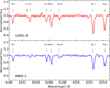 |
Fig. 1 Comparison between UVES-3 and MIKE-2 spectra after reduction, normalisation, radial velocity, and heliocentric corrections. The two stars share similar atmospheric parameters and iron abundances. Black ticks mark the position of observable lines. |
RV and atmospheric parameters of the observed SMC targets.
3.2 Atmospheric parameters
We computed the atmospheric parameters for the target stars from photometry (Table 2). Effective temperatures (Teff) were obtained from the broad-band colour (G−Ks)0, adopting the (G−Ks)0 − Teff transformation from Mucciarelli et al. (2021a), exploiting Gaia DR3 G magnitudes (Gaia Collaboration 2018), 2MASS Ks magnitudes (Skrutskie et al. 2006) and colour excess values E(B − V) from infrared dust maps (Schlafly & Finkbeiner 2011). The effective temperatures are characterised by uncertainties of ∼50 K, including the uncertainty of the calibration itself (the dominant source of error) and the errors in the G−Ks colour and in the colour excess.
The surface gravities (log g) were derived through the Stefan-Boltzmann relation, using the Teff values, a true distance modulus (m − M)0 = 18.965 ± 0.025 (Graczyk et al. 2014), bolometric corrections according to Andrae et al. (2018), and stellar masses of 0.75 ± 0.10 M⊙. The typical log g errors are of the order of 0.1.
Microturbulent velocities (vt) were computed using log g– vt relations from Mucciarelli & Bonifacio (2020), consistently with Paper I. The error associated to vt is about 0.2 km s−1, considering the quadrature sum of the uncertainties of the log g–vt relation and of log g itself. Paper I did not determine the vt values spectroscopically, in order to avoid large fluctuations, potentially caused by the small number of Fe I lines and weak lines of their GIRAFFE spectra. The new dataset of UVES and MIKE spectra allowed us to spectroscopically measure vt thanks to the large number (∼120 − 170) of available Fe I lines. The new values are fully consistent within the uncertainties with those derived from the log g–vt relations used above.
3.3 Radial velocities
We measured the radial velocities (RV) using the cross correlation function (CCF) technique (see e.g. Tonry & Davis 1979) as implemented in the PyAstronomy package. Templates are synthetic spectra calculated with SYNTHE (Sect. 3.1). The RV errors associated to this CCF measurements are of ∼0.02 km s−1 and were computed by means of MonteCarlo simulations. For each target, we added Poissonian noise to the appropriate synthetic spectrum, in order to simulate the S/N of our UVES/MIKE spectra, and then Gaussian fitted the main peak of the CCF resulting from the comparison between the observed and Poissonian noise synthetic spectra, and repeated this process 200 times. The standard deviation resulting from each set of RV values was used to derive the error on the RV measure procedure. However, the total error associated to our RV measurements was dominated by uncertainties of ∼0.5 km s−1 related to the stability of UVES/MIKE and their set-ups. We checked the wavelength calibration accuracy of UVES/MIKE spectra by measuring the position of 5577.3 Å and 6300.3 Å O I sky emission lines, finding shifts that were compatible with a zero velocity and ruling out significant systematics in the zero-points of the wavelength scale.
When compared against Paper I GIRAFFE measurements, the RV of our UVES targets show an average difference of −1.1±0.5 km s−1. MIKE targets RV show a much better agreement with their APOGEE DR17 (Abdurro’uf et al. 2022) RV measurements, with an average difference of 0.0 ± 0.5 km s−1. Looking at single targets, four of them from both sub-samples display absolute RV discrepancies larger than 1.5 km s−1 with respect to currently available RV estimates: atmospheric jitter caused by the extended convective structure and other instabilities in the observed RGB stars can account for such discrepancies.
3.4 Chemical abundances
The computation of chemical abundances for all absorption lines was done using the SALVADOR code (Alvarez Garay et al., in prep.), which performs a χ2-minimisation between an observed spectrum and a grid of synthetic spectra computed on the fly with the SYNTHE code around each absorption line. For the computation of C and N abundances for the targets observed with UVES, wider regions than the ones for single absorption lines from Blue Arm setting spectra were used, in order to correctly analyse the molecular absorption bands of CH and CN. Chemical abundances where computed using solar reference abundances from Grevesse & Sauval (1998), except for oxygen, for which we adopted the value by Caffau et al. (2011). NLTE corrections are often required for chemical abundances of some elements, especially in the case of metal-poor stars (Asplund 2005). In our analysis, we applied NLTE corrections by Mashonkina (2013) for Mg I lines, by Mashonkina et al. (2017) for Ca I lines, by Mashonkina et al. (2011) for Fe I lines, by Mashonkina & Belyaev (2019) for Ba II lines, and by Mashonkina & Gehren (2000) for Eu II lines. All corrections were applied using the database from Mashonkina et al. (2023).
Uncertainties in the computation of chemical abundances are caused by measurement errors and uncertainties from atmospheric parameters. The average abundance value from multiple absorption lines of the same element in a given star comes with a measurement error (i.e. the standard deviation of the mean abundance). These errors arise from the spectral fitting procedure and from the log g f values assumed for each absorption feature. In the case only one absorption feature of an element is available, its abundance measurement error was measured by running a Monte Carlo simulation of 200 synthetic spectra with the addition of Poissonian noise to reproduce the observed S/N. The single feature was analysed in each of these spectra with SALVADOR, and the standard deviation of the derived abundance distribution is assumed as the measurement error.
The uncertainties arising from atmospheric parameters were computed with additional analyses where the atmospheric parameters were changed, according to their 1σ errors (50 K for Teff, 0.1 for log g, 0.2 km s−1 for vt), one at a time, to evaluate the effect of each parameter uncertainty on the abundance computation.
These two sources of uncertainties were summed in quadrature to obtain the actual uncertainties associated to the measured abundances: this was done because we computed the covariance terms arising from Teff–log g (and, consequently, Teff–vt) and log g–vt relations, and we observed that they impact for <0.01 dex on the final error of our abundances. Uncertainties in the measured iron abundances are therefore given by the quadrature sum,
![Mathematical equation: ${\sigma _{[{\rm{Fe}}/{\rm{H}}]}} = \sqrt {{{\sigma _{{\rm{Fe}}}^2} \over {{N_{{\rm{Fe}}}}}} + {{\left( {\delta _{{\rm{Fe}}}^{{T_{{\rm{Fe}}}}}} \right)}^2} + {{\left( {\delta _{{\rm{Fe}}}^{\log g}} \right)}^2} + {{\left( {\delta _{{\rm{Fe}}}^{{v_{\rm{f}}}}} \right)}^2}} .$](/articles/aa/full_html/2026/02/aa57891-25/aa57891-25-eq1.png) (1)
(1)
For all the other elements, since their abundances are in the form [X/Fe], their uncertainties were consequently computed as
![Mathematical equation: $\eqalign{& {\sigma _{[{\rm{X}}/{\rm{Fe}}]}} = \cr & \sqrt {{{\sigma _{\rm{X}}^2} \over {{N_{\rm{X}}}}} + {{\sigma _{{\rm{Fe}}}^2} \over {{N_{{\rm{Fe}}}}}} + {{\left( {\delta _{\rm{X}}^{{T_{{\rm{eff}}}}} - \delta _{{\rm{Fe}}}^{{T_{{\rm{eff}}}}}} \right)}^2} + {{\left( {\delta _{\rm{X}}^{\log g} - \delta _{{\rm{Fe}}}^{\log g}} \right)}^2} + {{\left( {\delta _{\rm{X}}^{{v_t}} - \delta _{{\rm{Fe}}}^{{v_t}}} \right)}^2}} . \cr} $](/articles/aa/full_html/2026/02/aa57891-25/aa57891-25-eq2.png) (2)
(2)
In the two above formulas, σFe and σX are the standard deviations of Fe and X element abundances, respectively; NX and NFe are the number of fitted absorption lines used in the abundance measurement of Fe and the X element, respectively;  , Fe are the abundance variations caused by the variation of the atmospheric parameter, p.
4 Iron abundances
The iron abundances of the 12 SMC stars were derived from ∼150–170 Fe I lines. We also measured 15–20 Fe II lines, but in two metal-poor MIKE targets only 5 Fe II lines are available. Table 3 lists the average LTE and NLTE Fe abundances derived from neutral lines, along with the LTE abundance from single ionised lines (for the latter the NLTE effects are negligible because Fe II is the dominant ionisation stage). Because of the excellent agreement between the abundances from Fe I and Fe II lines and the higher precision of the [Fe/H] derived from the neutral lines (due to the huge number of used lines), we refer only to the NLTE [Fe/H] from Fe I lines in this work.
Our sample of SMC stars has −2.3 < [Fe/H] <−1.4 dex, with 10 out of 12 stars with [Fe/H] < −1.8 dex. The agemetallicity relation (AMR) from Pagel & Tautvaisiene (1998) allows us to provide an estimate of the age of these stars (see Fig. 2). In fact, according to this AMR, all our targets should be older than ∼11 Gyr. In particular, the two metal-rich targets should have an age between 11 and 12 Gyr, while the other ten stars should be formed in the first 1.5 Gyr of life of the galaxy. As a reference, we recall that the oldest SMC GC, NGC 121, has an age of 10.5±0.5 Gyr (Glatt et al. 2008), with [Fe/H] = −1.18 ± 0.02 dex (Paper II). Moreover, since all our targets show [Fe/H] < −1.4 dex, their formation should have occurred before the SMC quiescent phase, where a wide spread in ages (from 11 to 4 Gyr) corresponds to a rather small variation of iron, −1.3 < [Fe/H] < −1.2 dex. This occurs as a consequence of a low SFR, while this galaxy was also characterised by an inhomogeneous evolution.
The four SMC metal-poor stars analysed by R21 are in common with our sample (see Table 1). We compare our atmospheric parameters and [Fe/H] with those by R21. In their work, R21 determined both Teff and vt of their targets spectroscopically, while log g were derived using isochrones. The average differences are (< Teff − Teff, R21 >= −130 ± 60 K), (< log g − log gR21 >= −0.10 ± 0.06 in cgs units), and (< vt − vt, R21 >= −0.99 ± 0.18 km s−1). The latter difference is particularly significative and we attribute their large values of vt (3.0 km s−1 on average, which is unlikely for low-mass giant stars) to the spectroscopical determination of this parameter that is based on the balance of the abundances from weak and strong lines. The MIKE spectra analysed by R21 have relatively low S/N (∼45 at 6500 Å, ∼20 at 4500 Å, on average), thus introducing a bias against the weak lines that leads to spurious vt.
There is a significant offset of < [Fe/H] − [Fe/H]R21 >= +0.25 ± 0.06 dex between the two sets of abundances. Given the magnitude of NLTE corrections on Fe I lines, R21 preferred to use abundances from Fe II lines as their final [Fe/H] measurements. Even considering their [Fe/H] from Fe I lines, we still get a significant offset of < [Fe/H]−[Fe/H]R21 >= +0.26±0.08 dex; however, in this case, we are comparing our set of NLTE Fe I abundances with a LTE one. If we compare the two sets of LTE Fe I abundances, then the offset actually reduces to < [Fe/H]LTE−[Fe/H]R21 >= +0.18 ± 0.08 dex. We attribute this difference to the differences in vt and Teff.
The iron abundances we measured for UVES targets are compatible with their previous GIRAFFE measurements (Paper I), with an average difference < [Fe/H]UVES−[Fe/H]GIRAFFE >= 0.10 ± 0.08 dex. UVES-6 is the only target showing a significant difference ([Fe/H]UVES−[Fe/H]GIRAFFE = 0.55 ± 0.15 dex), likely due to the low spectral quality of the GIRAFFE spectra for this star. Finally, we compared [Fe/H] for MIKE targets with the values available in APOGEE DR17, finding an excellent agreement, with an average difference of < [Fe/H]MIKE−[Fe/H]APOGEE >= +0.04 ± 0.07 dex.
Fe I LTE, Fe I NLTE, and Fe II.
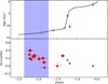 |
Fig. 2 Upper panel: theoretical AMR of the SMC (black line, Pagel & Tautvaisiene 1998), superimposed with the SMC GCs (Paper II, green circles). The white dots mark the position on the theoretical AMR of ages 11, 12 and 13 Gyr. Lower panel: average Si and Ca abundances as a function of [Fe/H] for SMC stars of this work observed with UVES (red squares) and MIKE (red triangles). The blue shaded area highlights the [Fe/H] region of the stars of our sample with −2.2 < [Fe/H] < −1.8 dex. |
5 Chemical abundance ratios
Here, we present chemical abundances for C, N, α-elements (O, Mg, Si, Ca), and neutron-capture elements (Y, Ba, La, Ce, Nd, Sm, Eu). For the latter, Ba and La were already measured in Paper I for the UVES targets, while no abundances are available from APOGEE for the MIKE targets. We show the abundances of the targets in a series of [X/Fe]-[Fe/H] abundance diagrams (Figs. 3–10), in comparison with the abundances of the SMC field stars (Paper I) and of the SMC globular clusters (Paper II). Additionally, we show abundance ratios for MW field stars from SAGA database (Suda et al. 2008). Since this database compiles results from different analyses, it is not fully homogeneous and should be considered in a statistical sense. Nevertheless, the overall trends of MW stars are a useful reference for a comparison with the SMC stars, despite the fact that this comparison can be affected by the systematics among the different analyses (in terms of model atmospheres, solar abundance values, NLTE corrections, line lists, and use of dwarf and giant stars).
5.1 Carbon and nitrogen
For cool stars such as the targets analysed here, the spectrum can be contaminated by several CN or CH molecular features; therefore, the use of appropriate C and N abundances is necessary in the evaluation of the level of blending of each feature. For the UVES targets only we measured C abundances from the CH G-band at 4300 Å and N abundances from the CN molecular band at 3880 Å. For the MIKE targets, the S/N at the wavelengths of the CH and CN molecular bands is too low to allow us a reliable measure; hence, we adopted [C/Fe] and [N/Fe] average values measured in the UVES targets for the spectral synthesis of the other elements. Since the main focus of this analysis is on α and neutron-capture elements, we provide more details about C and N abundances of our targets in Appendix B.
5.2 α-elements
We measured abundances for the α-elements O, Mg, Si, and Ca. Oxygen abundances were computed from the forbidden line at 6300.3 Å, cleaned from possible telluric contamination using appropriate synthetic spectra of the Earth atmosphere calculated with the tool TAPAS (Bertaux et al. 2014). Magnesium abundances were obtained from the Mg lines at 4167.3 Å and 5711.1 Å. Silicon abundances were based on the absorption features at 5948.5 Å and 6155.1 Å . Calcium abundances were derived from ∼15 Ca I lines. Figure 3 displays the run of the above mentioned [α/Fe] abundance ratios as a function of [Fe/H]. All the targets exhibit mildly enhanced [α/Fe] abundance ratios, about ∼+0.2 dex, apart from [O/Fe] that generally show higher values. In general, the SMC stars at these [Fe/H] have lower [α/Fe] than those measured in MW stars of similar [Fe/H], as found both from optical (Paper I) and near-infrared analyses (Nidever et al. 2020; Hasselquist et al. 2021, 2024).
5.3 r-process elements
We measured two neutron-capture elements mainly formed by the r-process, namely, europium (Eu, one of the purest r-process elements) and samarium (Sm), produced by the r-process at ≃65 % in the Solar System (Sneden et al. 2008).
We computed the Eu abundances from the Eu II line at 6645.1 Å (and from 6437.6 Å when visible). As shown in Fig. 4, our [Eu/Fe] abundances are indeed comparable with MW stars Eu content. The SMC targets also exhibit a large star-to-star scatter in [Eu/Fe], spanning ∼1 dex and larger than their uncertainties, which indicates an intrinsic scatter among our stars, in line with the first claim provided in Paper IV.
All [Eu/Fe] abundance ratios are supersolar, with the three highest [Eu/Fe] stars (UVES-1, UVES-6, MIKE-1) that can be classified as r-II stars (i.e. with [Eu/Fe] > +0.7, Holmbeck et al. 2020). These three r-II stars confirm that r-process synthesis can be extremely efficient in a galaxy such as the SMC, as already suggested by R21. Finally, we compared our [Eu/Fe] with those by R21 for the stars UVES-1 and UVES-5, finding an average difference <[Eu/Fe]−[Eu/Fe]R21 >= −0.23 ± 0.15 dex.
As for Sm, we identified few lines, always bluewards of 4950 Å. The [Sm/Fe] abundances we measured (Fig. 5) display a ∼1 dex wide star-to-star scatter as observed for [Eu/Fe]. In particular, four stars have high [Sm/Fe] (the same stars are also among the most Eu-rich targets), while the other stars shows a mild decrease of [Sm/Fe] by increasing [Fe/H]. As expected due to the common r-process origin, we find correspondence between Sm and Eu contents: the stars with the highest (lowest) [Sm/Fe] abundances are those with the highest (lowest) [Eu/Fe].
5.4 s-process elements
We measured a number of neutron-capture elements that are primarily formed through the s-process at solar metallicity, namely, Y (belonging to the first peak of s-process), as well as Ba, La, Ce, and Nd (belonging to the second peak).
As for the Y abundances, they were based on 4–12 Y II lines, depending on the target. Figure 6 shows the SMC stars [Y/Fe] abundances that appear to be, on average, lower than the MW stars of similar [Fe/H].
Barium is a second-peak s-process element, mainly produced in AGB stars generally below 4 M⊙ (Gallino et al. 1998), with yields highly dependent on metallicities and only in minor amount in fast-rotating massive stars. We measured [Ba/Fe] from Ba II lines at 4934.1 Å, 5853.7 Å, 6141.7 Å, 6496.9 Å. Since some of these features are often saturated, the abundances obtained from their profiles should be handled with care and their uncertainties are more sensitive to the adopted values, in particular of microturbulence, in model atmosphere. Figure 7 highlights that our [Ba/Fe] are indeed comparable with Galactic values. However, two stars (UVES-1 and MIKE-1) stand out from other SMC metal-poor stars, at clearly higher [Ba/Fe]: we point out how UVES-1 and MIKE-1 also are the two stars with the highest [Eu/Fe].
We measured the La abundances relying on ∼10 La II lines in UVES spectra and only few lines in MIKE spectra. Contrarily to barium, nearly half of the sample is depleted in [La/Fe] with respect to Galactic values (Fig. 8). Five out of the six stars with the highest (supersolar) [La/Fe] have [Eu/Fe] > +0.5: the stars with the highest [La/Fe] are indeed the stars with the highest [Eu/Fe].
With respect to Ce, only a few Ce II lines are visible, mainly in regions bluewards of 4650 Å. The [Ce/Fe] abundances of 8 out of 12 metal-poor SMC stars are depleted with respect to MW stars at similar [Fe/H] (Fig. 9). Most of our targets have sub-solar [Ce/Fe] values, comparable with APOGEE [Ce/Fe] abundances (Hasselquist et al. 2021). Once again, the three stars with super-solar and highest [Ce/Fe] of our sample (UVES-1, UVES-6, MIKE-1) are indeed the three r-II stars we mentioned previously.
We determined the Nd abundances from ∼15 Nd II lines per UVES spectra and only few per MIKE spectra. The obtained [Nd/Fe] abundances are generally solar or sub-solar and slightly lower than Galactic stars of similar [Fe/H] (Fig. 10). Again, the four stars (UVES-1, UVES-6, MIKE-1, MIKE-5) with the highest [Nd/Fe] all have [Eu/Fe] >+0.6; whereas the three stars (UVES-4, UVES-7, MIKE-4) with the lowest [Nd/Fe] are indeed the stars with the lowest [Eu/Fe] of the entire SMC sample.
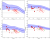 |
Fig. 3 α-elements patterns: [O/Fe], [Mg/Fe], [Si/Fe], and [Ca/Fe] abundances as a function of [Fe/H] for SMC stars of this work observed with UVES (red squares) and MIKE (red triangles), together with the SMC field stars (Paper I, red small circles) and the SMC GCs (Paper II, green circles). Error bars are shown for UVES and MIKE abundances. As a reference, Gaussian KDE regressions of MW abundances built from SAGA database (Suda et al. 2008) (blue line) are reported, together with their 1σ confidence interval (blue shaded area), in the background. |
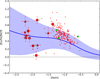 |
Fig. 4 [Eu/Fe] abundances as a function of [Fe/H]. Same symbols as in Fig. 3, but the red small circles are SMC field stars observed with GIRAFFE from Paper IV. |
6 The early chemical enrichment of the SMC
As pointed out in Sect. 4, the [Fe/H] results suggest most of the observed stars are likely >12 Gyr old according to the SMC AMR models. In particular, stars with [Fe/H] < −1.8 stars must have formed in the first Gyr of life of the SMC. These stars show mildly enhanced [α/Fe] ratios indicating a major contribution by CC-SNe. In fact, the main site of production of α-elements are massive stars ending their evolution after few tens million years with CC-SNe explosion, while there is just a marginal contribution from SNe Ia explosions. The delay between the enrichment timescales of CC-SNe and SNe Ia explains the behaviour of [α/Fe] as a function of [Fe/H] (Tinsley 1979; Matteucci & Greggio 1986). However, the values of [α/Fe] in these stars are on average lower than those usually measured in MW stars of similar [Fe/H], as already pointed out by Nidever et al. (2020), Hasselquist et al. (2021) and Paper I. This suggests a lower contribution to the early chemical enrichment of the SMC by massive stars and likely a α-knee occurring at lower metallicities. This finding is in line with the lower SFR of the SMC with respect to the MW (Cignoni et al. 2012, 2013; Rubele et al. 2018; Massana et al. 2022).
By that time (in the first Gyr of the SMC life), most low-mass stars could not have evolved up to AGB phase and could not have already enriched the SMC gas with their s-process signature. In contrast to what happens at higher metallicities, namely, at later times in the chemical evolution of a galaxy, the so called s-process elements actually lack their main channel of formation down to [Fe/H] ∼ − 2.0 (while also considering that even the few AGB stars have metallicity values for which s-process nucle-osynthesis is disfavoured). Within this scenario, the r-process eventually become the main channel of nucleosynthesis for all neutron-capture elements (Truran 1981) and we expect to see the patterns and features of r-process elements (Eu, Sm) in the ‘s-process’ elements (Y, Ba, La, Ce, and Nd) as well.
Indeed, if we compare the abundances of [Eu/Fe] or [Sm/Fe] (Figs. 4 and 5) with any of the observed s-process elements (Figs. 6–10), we note that all these abundances share a similar ∼1 dex wide scatter in [X/Fe]. The large star-to-star [Eu/Fe] scatter among metal-poor Galactic stars (and in a similar way in the SMC) is caused by the rarity of events like NSM producing r-process elements. On the other hand, the metal-richer decrease of [Eu/Fe] is the result of the same delayed chemical contribution from SNe Ia at the basis of the decline of [α/Fe]: in fact, SNe Ia are not expected to produce r-process elements, while they mainly inject iron-peak elements in the gas.
Moreover, as highlighted for multiple elements in Sect. 5.4, whenever a star has high [Eu/Fe] (or also [Sm/Fe]), it also shows high values of [s/Fe]. A comparison between [s/Eu] and [Fe/H] better represents the previous statement. In Fig. 11, it is possible to see that, independently of the metallicity of our metal-poor stars, [s/Eu] abundances stand at a fairly constant level despite their scatter, very similarly to [Sm/Eu]. We see that s-elements in the SMC have been produced at a constant ratio with Eu/r-process elements throughout the −2.3 < [Fe/H] < −1.4 range and they show consistently (and often markedly) sub-solar values. These two features are clearly showing the r-processes are driving the nucleosynthesis of all the analysed neutron-capture elements, while suggesting no relevant s-process acting at this metallicities, with only possible small s-process contribution from rotating massive stars.
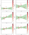 |
Fig. 11 [Y/Eu], [Ba/Eu], [La/Eu], [Ce/Eu], [Nd/Eu] and [Sm/Eu] abundances as a function of [Fe/H] for SMC stars observed with UVES (squares) and MIKE (triangles). Points are coloured according to their [Eu/Fe] abundances. Lower limits are reported with arrows. In each plot, the linear regression of the measured abundances and their 95% confidence intervals are shown with a green dashed line and green shaded area, respectively. |
7 Comparison with a stochastic chemical evolution model for the SMC
To test our claims on more theoretical grounds, we adopted a stochastic chemical evolution model to describe the early chemical evolution in the SMC, as detailed in this section. The model resembles the scheme adopted in the stochastic models presented in Cescutti (2008); Cescutti & Chiappini (2010) and later adopted in other works to model the early evolution of the Galactic halo. Stochasticity is introduced by dividing the galaxy into isolated cubic regions, each containing the typical mass of gas swept by a CC-SNe (see Cescutti 2008). Within each cubic region, the model considers at each step gas inflow and outflow, gas recycling due to evolving stars and star formation. For the latter, masses of the stars formed are randomly extracted weighting them according to the initial mass function (here Scalo 1986). More details on the physical prescriptions adopted in the model are given in Appendix C.1. However, it is worth to point out that to model the chemical evolution of the SMC, we adopted a smaller value of the star formation efficiency (SFE) to what is routinely adopted for the MW halo (i.e. ν = 0.25 Gyr−1). The latter value is in line with values usually adopted to model the evolution of the MCs (see, e.g. Vasini et al. 2023). Adopting this prescription for the SF, we sampled a number of 100 volumes, which resulted in a summed total mass at the end of the run (of 1.5 Gyr) of ∼2 × 10⁷ M⊙, similar to the stellar mass inferred from CMD fitting in the same age range by Massana et al. (2022, ∼5 × 10⁷ M⊙).
To trace the evolution of neutron-capture elements, the model includes different sources for both s-process and r-process synthesis. The s-process is synthesised in rotating massive stars and AGB stars, for which we adopted the stellar yields by Limongi & Chieffi (2018, adopting the rotational velocity distribution by Rizzuti et al. 2021) and the FRUITY database (e.g. Cristallo et al. 2011), respectively. The r-process is instead competitively produced in MRD-SNe and NSM in the model. For MRD-SNe, we adopted the yields of Nishimura et al. (2017) and a fraction in the progenitor mass range of 0.1. For NSM, we adopt the same yields as in Molero et al. (2023, derived from Sr measurement in the Kilonova AT2017gfo, Watson et al. 2019), a binary fraction in the progenitor range of 0.08 (as derived in Palla et al. 2025) and a fixed coalescence timescale of 100 Myr. This timescale is set to distinguish clearly the effect between the prompt (MRD-SNe) and the delayed (NSM) source of r-process production. For further details on the nucleosynthesis prescriptions, we refer to Appendix C.1.
In Fig. 12, we show the output of our fiducial stochastic chemical evolution model with the [Eu/Fe] abundances derived for metal-poor SMC stars. The observations are aptly reproduced by the stochastic model, which also reflects the abundance spread observed in stars in our sample. In turn, this confirm our indication that such a spread of ∼1 dex in [Eu/Fe] is a consequence of inhomogeneous mixing in the early evolution of the SMC, analogously to what is observed in the MW at similar metallicities (see Fig. 4). However, to achieve the result in Fig. 12, in the SMC model we have to increase significantly the fraction of system originating NSM relative to Galactic studies. Indeed the adopted fraction for the MW spans a range between 2 × 10⁻³ and 0.02 (e.g. Molero et al. 2021, 2023; Cavallo et al. 2021), whereas here we adopted 0.08, according to the hypothesis by Palla et al. (2025) of a larger fraction of NSM progenitor to reproduce MW satellite europium patterns at low metallicity. It is worth noting that to probe the effect of NSM progenitor fraction in the early SMC evolution, we run an additional model with lower fraction of NSM progenitor (6 × 10⁻³, in the range of values adopted for the MW). The comparison between the two models is shown in Fig. C.2 and shows clearly the need for a large fraction of NSM at low-metallicity to reproduce the upper envelope of [Eu/Fe] abundances, indicating a higher relative rate of r-process events in the Cloud.
In Fig. 13, we show instead the comparison between our fiducial stochastic chemical evolution model and SMC stars for [Ba/Fe], being Ba a typical s-process element. In particular, Fig. 13 left panel shows the predicted density of long-lived stars, while right panel displays the fraction of Ba abundance produced by the s-process (both from AGBs and rotating massive stars). The two panels show clearly that in order reproduce the pattern and spread of SMC metal-poor stars we need that the majority of Ba production comes from the r-process: low-mass AGB stars do not have sufficient time to pollute the ISM at these early stages of evolution, while rotating massive stars are responsible of the low-metallicity, [Ba/Fe]-poor end of the predictions, where no data were found. This strikingly highlights the claim of r-process driven production for neutron-capture elements in the SMC brought out in Sect. 6. Moreover, further tests on enhanced and more significant s-process production from rotating massive stars reveal this scenario to be unlikely. Indeed, adopting a rotational velocity distribution more in favour of rapidly rotating stars relative to the fiducial one (see Figure C.3) leads to an extreme enhancement in Ba (≳0.5 dex at [Fe/H] ∼ −1.5 dex), which is not followed by the data trend.
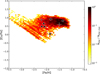 |
Fig. 12 [Eu/Fe] abundances as a function of [Fe/H] as predicted by our adopted stochastic chemical evolution model. The colormap displays the number density of predicted long-lived stars by the model on a logarithmic scale. Observed SMC abundances with relative errorbar are represented with black symbols (squares: UVES observations, triangles: MIKE observations). |
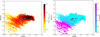 |
Fig. 13 [Ba/Fe] abundances as a function of [Fe/H] as predicted by our adopted stochastic chemical evolution model. On the left panel, the colormap displays the number density of predicted long-lived stars by the model on a logarithmic scale. On the right panel, the colormap displays the fraction of element abundance produced by s-process over total. Black symbols are as in Fig. 12. |
8 Conclusions
We analysed high-resolution UVES and MIKE spectra for 12 metal-poor SMC RGB stars focussing on their abundances of neutron-capture elements (in particular the pure r-process elements Eu and Sm). The main results emerging from this chemical analysis are summarised in the following:
The targets are characterised by [Fe/H] values between −2.3 and −1.4 dex, 10 out 12 with [Fe/H] <−1.8 dex. According to the theoretical AMR from Pagel & Tautvaisiene (1998), these stars formed in the first Gyr of life of the SMC;
The α-elements are enhanced in metal-poor SMC stars, but at a lower level with respect to MW stars of similar [Fe/H]. This lower [α/Fe] enhancement and a mild decrease of [α/Fe] for increasing metallicity are consistent with the SFR of the SMC, less efficient than that of the MW. This dataset suggests that the α-knee occurs at lower [Fe/H] than in the MW, but it is not yet possible to properly identify it. This is visible in Fig. 3: metal-poor SMC stars draw a decreasing trend reaching solar or occasionally mildly sub-solar [α/Fe] both in hydrostatic (Mg and O) and in explosive (Si and Ca) α-elements;
The targets cover a large range of [Eu/Fe], from solar values up to ∼+1 dex, with three stars showing [Eu/Fe] > +0.7. This large star-to-star scatter, not explicable within the uncertainties, is similar to that observed in metal-poor MW stars. Analogue pattern is observed for [Sm/Fe]. Such pattern indicates that the r-process in the SMC can be extremely efficient (as claimed in R21), but still largely affected by the stochastic nature of the main sites of production and inefficient gas mixing in the early SMC evolution. These findings are in line with predictions from a stochastic chemical evolution model simulating the early evolution of the SMC;
In addition, the s-process elements show large star-to-star scatter not compatible within the uncertainties. Whenever a star has high [Eu/Fe], it also shows high [s/Fe]. Moreover, we observe all stars have markedly sub-solar [s/Eu]. At these metallicities, the nucleosynthesis of the neutron-capture elements is driven by r-processes, since the low-mass AGB stars have not yet evolved and left their s-process signature in the ISM. This interpretation is confirmed by results of the stochastic chemical evolution model, also suggesting that s-process production in rotating massive stars can only account for a very minor fraction of the abundance in the observed stars.
In summary, the SMC metal-poor stars display distinct [α/Fe] with respect to MW metal-poor stars. Indeed, the α patterns suggest the SMC has a lower SFR than the MW, leading to a lower contribution by massive stars to the overall chemical enrichment of the galaxy (Matteucci 2012). On the other hand, all neutron-capture elements, including those usually identified as s-process, are mostly driven by r-process production, exhibiting the typical characteristics (i.e. scatter and relative abundances) of r-process nucleosynthesis.
Acknowledgements
A.M., M.P. and D.R. acknowledge support from the project “LEGO – Reconstructing the building blocks of the Galaxy by chemical tagging” (P.I. A. Mucciarelli) granted by the Italian MUR through contract PRIN 2022LLP8TK_001. L.M. gratefully acknowledges support from ANID-FONDECYT Regular Project no. 1251809. D.A.A.G. acknowledges funding from the European Union under the grant ERC-2022-AdG, ‘StarDance: the non-canonical evolution of stars in clusters’, Grant Agreement 101093572, PI: E. Pancino.
References
- Abdurro’uf, Accetta, K., Aerts, C., et al. 2022, ApJS, 259, 35 [NASA ADS] [CrossRef] [Google Scholar]
- Andrae, R., Fouesneau, M., Creevey, O., et al. 2018, A&A, 616, A8 [NASA ADS] [CrossRef] [EDP Sciences] [Google Scholar]
- Anoardo, S., Mucciarelli, A., Palla, M., et al. 2026, A&A, 705, A31 [NASA ADS] [CrossRef] [EDP Sciences] [Google Scholar]
- Argast, D., Samland, M., Thielemann, F. K., & Qian, Y. Z. 2004, A&A, 416, 997 [NASA ADS] [CrossRef] [EDP Sciences] [Google Scholar]
- Asplund, M. 2005, ARA&A, 43, 481 [Google Scholar]
- Bernstein, R., Shectman, S. A., Gunnels, S. M., Mochnacki, S., & Athey, A. E. 2003, SPIE, 4841, 1694 [NASA ADS] [Google Scholar]
- Bertaux, J. L., Lallement, R., Ferron, S., Boonne, C., & Bodichon, R. 2014, A&A, 564, A46 [NASA ADS] [CrossRef] [EDP Sciences] [Google Scholar]
- Biémont, É., Blagoev, K., Engström, L., et al. 2011, MNRAS, 414, 3350 [Google Scholar]
- Bonifacio, P., Caffau, E., François, P., & Spite, M. 2025, A&A Rev., 33, 2 [Google Scholar]
- Burbidge, E. M., Burbidge, G. R., Fowler, W. A., & Hoyle, F. 1957, Rev. Mod. Phys., 29, 547 [NASA ADS] [CrossRef] [Google Scholar]
- Caffau, E., Ludwig, H. G., Steffen, M., Freytag, B., & Bonifacio, P. 2011, Sol. Phys., 268, 255 [Google Scholar]
- Cameron, A. G. W. 1957, PASP, 69, 201 [NASA ADS] [CrossRef] [Google Scholar]
- Carrera, R., Gallart, C., Aparicio, A., et al. 2008, AJ, 136, 1039 [Google Scholar]
- Castelli, F., & Kurucz, R. L. 2003, 210, IAU Symp., 210, A20 [Google Scholar]
- Cavallo, L., Cescutti, G., & Matteucci, F. 2021, MNRAS, 503, 1 [CrossRef] [Google Scholar]
- Cescutti, G. 2008, A&A, 481, 691 [NASA ADS] [CrossRef] [EDP Sciences] [Google Scholar]
- Cescutti, G., & Chiappini, C. 2010, A&A, 515, A102 [NASA ADS] [CrossRef] [EDP Sciences] [Google Scholar]
- Chiti, A., Mardini, M., Limberg, G., et al. 2024, Nat. Astron., 8, 637 [NASA ADS] [CrossRef] [Google Scholar]
- Cignoni, M., Cole, A. A., Tosi, M., et al. 2012, ApJ, 754, 130 [NASA ADS] [CrossRef] [Google Scholar]
- Cignoni, M., Cole, A. A., Tosi, M., et al. 2013, ApJ, 775, 83 [Google Scholar]
- Clayton, D. D. 1968, Principles of Stellar Evolution and Nucleosynthesis (McGraw-Hill) [Google Scholar]
- Cowan, J. J., & Rose, W. K. 1977, ApJ, 212, 149 [Google Scholar]
- Cowan, J. J., Sneden, C., Lawler, J. E., et al. 2021, Rev. Mod. Phys., 93, 015002 [Google Scholar]
- Cristallo, S., Piersanti, L., Straniero, O., et al. 2011, ApJS, 197, 17 [NASA ADS] [CrossRef] [Google Scholar]
- Dekker, H., D’Odorico, S., Kaufer, A., Delabre, B., & Kotzlowski, H. 2000, SPIE, 4008, 534 [Google Scholar]
- Den Hartog, E. A., Lawler, J. E., Sneden, C., & Cowan, J. J. 2003, ApJS, 148, 543 [Google Scholar]
- Den Hartog, E. A., Ruffoni, M. P., Lawler, J. E., et al. 2014, ApJS, 215, 23 [NASA ADS] [CrossRef] [Google Scholar]
- Den Hartog, E. A., Lawler, J. E., Sneden, C., et al. 2021, ApJS, 255, 27 [NASA ADS] [CrossRef] [Google Scholar]
- Den Hartog, E. A., Lawler, J. E., Sneden, C., Roederer, I. U., & Cowan, J. J. 2023, ApJS, 265, 42 [Google Scholar]
- Frebel, A., Norris, J. E., Gilmore, G., & Wyse, R. F. G. 2016, ApJ, 826, 110 [NASA ADS] [CrossRef] [Google Scholar]
- Fuhr, J. R., & Wiese, W. L. 2006, J. Phys. Chem. Ref. Data, 35, 1669 [CrossRef] [Google Scholar]
- Fuhr, J. R., Martin, G. A., & Wiese, W. L. 1988, J. Phys. Chem. Ref. Data, 17 [Google Scholar]
- Gaia Collaboration (Babusiaux, C., et al.) 2018, A&A, 616, A10 [NASA ADS] [CrossRef] [EDP Sciences] [Google Scholar]
- Gallino, R., Arlandini, C., Busso, M., et al. 1998, ApJ, 497, 388 [Google Scholar]
- Gibson, B. K. 1997, MNRAS, 290, 471 [NASA ADS] [Google Scholar]
- Glatt, K., Gallagher, J. S. III, Grebel, E. K., et al. 2008, AJ, 135, 1106 [NASA ADS] [CrossRef] [Google Scholar]
- Graczyk, D., Pietrzyński, G., Thompson, I. B., et al. 2014, ApJ, 780, 59 [Google Scholar]
- Gratton, R. G., Sneden, C., Carretta, E., & Bragaglia, A. 2000, A&A, 354, 169 [NASA ADS] [Google Scholar]
- Gray, D. F. 2005, The Observation and Analysis of Stellar Photospheres (Cambridge University Press) [Google Scholar]
- Grevesse, N., & Sauval, A. J. 1998, Space Sci. Rev., 85, 161 [Google Scholar]
- Grichener, A., & Soker, N. 2019, ApJ, 878, 24 [Google Scholar]
- Hasselquist, S., Hayes, C. R., Lian, J., et al. 2021, ApJ, 923, 172 [NASA ADS] [CrossRef] [Google Scholar]
- Hasselquist, S., Hayes, C. R., Griffith, E. J., et al. 2024, ApJ, 974, 227 [Google Scholar]
- Holmbeck, E. M., Hansen, T. T., Beers, T. C., et al. 2020, ApJS, 249, 30 [NASA ADS] [CrossRef] [Google Scholar]
- Iben, I. Jr., & Renzini, A. 1983, ARA&A, 21, 271 [Google Scholar]
- Iwamoto, K., Brachwitz, F., Nomoto, K., et al. 1999, ApJS, 125, 439 [NASA ADS] [CrossRef] [Google Scholar]
- Johnson, J. A., Ivans, I. I., & Stetson, P. B. 2006, ApJ, 640, 801 [NASA ADS] [CrossRef] [Google Scholar]
- Käppeler, F., Gallino, R., Bisterzo, S., & Aoki, W. 2011, Rev. Mod. Phys., 83, 157 [Google Scholar]
- Karakas, A. I., & Lattanzio, J. C. 2014, PASA, 31, e030 [NASA ADS] [CrossRef] [Google Scholar]
- Kelson, D. D. 2003, PASP, 115, 688 [NASA ADS] [CrossRef] [Google Scholar]
- Kennicutt, Robert C.J., 1998, ApJ, 498, 541 [NASA ADS] [CrossRef] [Google Scholar]
- Klose, J. Z., Fuhr, J. R., & Wiese, W. L. 2002, J. Phys. Chem. Ref. Data, 31, 217 [Google Scholar]
- Kobayashi, C., Karakas, A. I., & Lugaro, M. 2020, ApJ, 900, 179 [Google Scholar]
- Kurucz, R. L. 2005, Mem. Soc. Astron. Ital. Suppl., 8, 14 [Google Scholar]
- Lagarde, N., Decressin, T., Charbonnel, C., et al. 2012, A&A, 543, A108 [NASA ADS] [CrossRef] [EDP Sciences] [Google Scholar]
- Lattimer, J. M., & Schramm, D. N. 1974, ApJ, 192, L145 [NASA ADS] [CrossRef] [Google Scholar]
- Lawler, J. E., Bonvallet, G., & Sneden, C. 2001a, ApJ, 556, 452 [NASA ADS] [CrossRef] [Google Scholar]
- Lawler, J. E., Wickliffe, M. E., den Hartog, E. A., & Sneden, C. 2001b, ApJ, 563, 1075 [CrossRef] [Google Scholar]
- Lawler, J. E., Den Hartog, E. A., Sneden, C., & Cowan, J. J. 2006, ApJS, 162, 227 [Google Scholar]
- Lawler, J., Sneden, C., Cowan, J. J., Ivans, I. I., & Den Hartog, E. A. 2009, in American Astronomical Society Meeting Abstracts, 213, 407.07 [Google Scholar]
- Limongi, M., & Chieffi, A. 2018, ApJS, 237, 13 [NASA ADS] [CrossRef] [Google Scholar]
- Manea, C., Ness, M., Hawkins, K., et al. 2025, ApJ, 993, 45 [Google Scholar]
- Mashonkina, L. 2013, A&A, 550, A28 [NASA ADS] [CrossRef] [EDP Sciences] [Google Scholar]
- Mashonkina, L. I., & Belyaev, A. K. 2019, Astron. Lett., 45, 341 [NASA ADS] [CrossRef] [Google Scholar]
- Mashonkina, L., & Gehren, T. 2000, A&A, 364, 249 [NASA ADS] [Google Scholar]
- Mashonkina, L., Gehren, T., Shi, J. R., Korn, A. J., & Grupp, F. 2011, A&A, 528, A87 [NASA ADS] [CrossRef] [EDP Sciences] [Google Scholar]
- Mashonkina, L., Sitnova, T., & Belyaev, A. K. 2017, A&A, 605, A53 [NASA ADS] [CrossRef] [EDP Sciences] [Google Scholar]
- Mashonkina, L., Pakhomov, Y., Sitnova, T., et al. 2023, MNRAS, 524, 3526 [Google Scholar]
- Massana, P., Ruiz-Lara, T., Noël, N. E. D., et al. 2022, MNRAS, 513, L40 [CrossRef] [Google Scholar]
- Matteucci, F. 2012, Chemical Evolution of Galaxies (Springer-Verlag) [Google Scholar]
- Matteucci, F., & Greggio, L. 1986, A&A, 154, 279 [NASA ADS] [Google Scholar]
- Matteucci, F., & Recchi, S. 2001, ApJ, 558, 351 [NASA ADS] [CrossRef] [Google Scholar]
- Meléndez, J., & Barbuy, B. 2009, A&A, 497, 611 [NASA ADS] [CrossRef] [EDP Sciences] [Google Scholar]
- Molero, M., Simonetti, P., Matteucci, F., & della Valle, M. 2021, MNRAS, 500, 1071 [Google Scholar]
- Molero, M., Magrini, L., Matteucci, F., et al. 2023, MNRAS, 523, 2974 [NASA ADS] [CrossRef] [Google Scholar]
- Mucciarelli, A. 2013, arXiv e-prints [arXiv:1311.1403] [Google Scholar]
- Mucciarelli, A., & Bonifacio, P. 2020, A&A, 640, A87 [NASA ADS] [CrossRef] [EDP Sciences] [Google Scholar]
- Mucciarelli, A., Origlia, L., & Ferraro, F. R. 2010, ApJ, 717, 277 [NASA ADS] [CrossRef] [Google Scholar]
- Mucciarelli, A., Pancino, E., Lovisi, L., Ferraro, F. R., & Lapenna, E. 2013, ApJ, 766, 78 [NASA ADS] [CrossRef] [Google Scholar]
- Mucciarelli, A., Bellazzini, M., & Massari, D. 2021a, A&A, 653, A90 [NASA ADS] [CrossRef] [EDP Sciences] [Google Scholar]
- Mucciarelli, A., Massari, D., Minelli, A., et al. 2021b, Nat. Astron., 5, 1247 [NASA ADS] [CrossRef] [Google Scholar]
- Mucciarelli, A., Minelli, A., Bellazzini, M., et al. 2023a, A&A, 671, A124 [NASA ADS] [CrossRef] [EDP Sciences] [Google Scholar]
- Mucciarelli, A., Minelli, A., Lardo, C., et al. 2023b, A&A, 677, A61 [NASA ADS] [CrossRef] [EDP Sciences] [Google Scholar]
- Mucciarelli, A., Bonifacio, P., & Lardo, C. 2026, A&A, 705, A134 [NASA ADS] [CrossRef] [EDP Sciences] [Google Scholar]
- Nidever, D. L., Hasselquist, S., Hayes, C. R., et al. 2020, ApJ, 895, 88 [Google Scholar]
- Nishimura, N., Sawai, H., Takiwaki, T., Yamada, S., & Thielemann, F. K. 2017, ApJ, 836, L21 [CrossRef] [Google Scholar]
- Nishimura, N., Takiwaki, T., & Thielemann, F.-K. 2015, ApJ, 810, 109 [Google Scholar]
- Oh, W. S., Nordlander, T., Da Costa, G. S., Bessell, M. S., & Mackey, A. D. 2024, MNRAS, 528, 1065 [NASA ADS] [CrossRef] [Google Scholar]
- Pagel, B. E. J., & Tautvaisiene, G. 1998, MNRAS, 299, 535 [Google Scholar]
- Palla, M., Molero, M., Romano, D., & Mucciarelli, A. 2025, A&A, 699, A209 [NASA ADS] [CrossRef] [EDP Sciences] [Google Scholar]
- Pehlivan Rhodin, A., Hartman, H., Nilsson, H., & Jönsson, P. 2017, A&A, 598, A102 [NASA ADS] [CrossRef] [EDP Sciences] [Google Scholar]
- Prantzos, N., Abia, C., Limongi, M., Chieffi, A., & Cristallo, S. 2018, MNRAS, 476, 3432 [Google Scholar]
- Reggiani, H., Schlaufman, K. C., Casey, A. R., Simon, J. D., & Ji, A. P. 2021, AJ, 162, 229 [NASA ADS] [CrossRef] [Google Scholar]
- Rizzuti, F., Cescutti, G., Matteucci, F., et al. 2021, MNRAS, 502, 2495 [NASA ADS] [CrossRef] [Google Scholar]
- Romano, D., Chiappini, C., Matteucci, F., & Tosi, M. 2005, A&A, 430, 491 [NASA ADS] [CrossRef] [EDP Sciences] [Google Scholar]
- Romano, D., Matteucci, F., Zhang, Z.-Y., Ivison, R. J., & Ventura, P. 2019, MNRAS, 490, 2838 [NASA ADS] [CrossRef] [Google Scholar]
- Rubele, S., Pastorelli, G., Girardi, L., et al. 2018, MNRAS, 478, 5017 [NASA ADS] [CrossRef] [Google Scholar]
- Ruffoni, M. P., Den Hartog, E. A., Lawler, J. E., et al. 2014, MNRAS, 441, 3127 [NASA ADS] [CrossRef] [Google Scholar]
- Ryde, N., Edvardsson, B., Gustafsson, B., et al. 2009, A&A, 496, 701 [NASA ADS] [CrossRef] [EDP Sciences] [Google Scholar]
- Salaris, M., Pietrinferni, A., Piersimoni, A. M., & Cassisi, S. 2015, A&A, 583, A87 [NASA ADS] [CrossRef] [EDP Sciences] [Google Scholar]
- Sbordone, L., Bonifacio, P., Castelli, F., & Kurucz, R. L. 2004, Mem. Soc. Astron. Ital. Suppl., 5, 93 [Google Scholar]
- Scalo, J. M. 1986, Fund. Cosmic Phys., 11, 1 [NASA ADS] [EDP Sciences] [Google Scholar]
- Schaller, G., Schaerer, D., Meynet, G., & Maeder, A. 1992, A&AS, 96, 269 [Google Scholar]
- Schlafly, E. F., & Finkbeiner, D. P. 2011, ApJ, 737, 103 [Google Scholar]
- Shectman, S. A., & Johns, M. 2003, SPIE, 4837, 910 [Google Scholar]
- Siegel, D. M., Barnes, J., & Metzger, B. D. 2019, Nature, 569, 241 [Google Scholar]
- Simon, J., Fu, S. W., Geha, M., Kelson, D. D., & Alarcon Jara, A. G. 2019, in American Astronomical Society Meeting Abstracts, 233, 449.04 [Google Scholar]
- Skrutskie, M. F., Cutri, R. M., Stiening, R., et al. 2006, AJ, 131, 1163 [NASA ADS] [CrossRef] [Google Scholar]
- Smith, V. V., Bizyaev, D., Cunha, K., et al. 2021, AJ, 161, 254 [NASA ADS] [CrossRef] [Google Scholar]
- Sneden, C., Cowan, J. J., & Gallino, R. 2008, ARA&A, 46, 241 [Google Scholar]
- Spite, M., Cayrel, R., Plez, B., et al. 2005, A&A, 430, 655 [NASA ADS] [CrossRef] [EDP Sciences] [Google Scholar]
- Stetson, P. B., & Pancino, E. 2008, PASP, 120, 1332 [Google Scholar]
- Straniero, O., Gallino, R., & Cristallo, S. 2006, Nucl. Phys. A, 777, 311 [NASA ADS] [CrossRef] [Google Scholar]
- Suda, T., Katsuta, Y., Yamada, S., et al. 2008, PASJ, 60, 1159 [NASA ADS] [Google Scholar]
- Tafelmeyer, M., Jablonka, P., Hill, V., et al. 2010, A&A, 524, A58 [CrossRef] [EDP Sciences] [Google Scholar]
- Thornton, K., Gaudlitz, M., Janka, H. T., & Steinmetz, M. 1998, ApJ, 500, 95 [CrossRef] [Google Scholar]
- Tinsley, B. M. 1979, ApJ, 229, 1046 [Google Scholar]
- Tonry, J., & Davis, M. 1979, AJ, 84, 1511 [Google Scholar]
- Truran, J. W. 1981, A&A, 97, 391 [NASA ADS] [Google Scholar]
- Ulrich, R. K. 1973, in Explosive Nucleosynthesis, eds. D. N. Schramm, & W. D. Arnett, 139 [Google Scholar]
- Vasini, A., Matteucci, F., Spitoni, E., & Siegert, T. 2023, MNRAS, 523, 1153 [NASA ADS] [CrossRef] [Google Scholar]
- Watson, D., Hansen, C. J., Selsing, J., et al. 2019, Nature, 574, 497 [NASA ADS] [CrossRef] [Google Scholar]
- Wiese, W. L., & Martin, G. A. 1980, Wavelengths and transition probabilities for atoms and atomic ions: Part 2. Transition probabilities, V68 [Google Scholar]
- Wiese, W. L., Fuhr, J. R., & Deters, T. M. 1996, Atomic transition probabilities of carbon, nitrogen, and oxygen : a critical data compilation (AIP Press) [Google Scholar]
Other secondary neutron-capture processes have also been identified, the most relevant being the intermediate process (Cowan & Rose 1977).
in Rizzuti et al. (2021), they adopt a Gaussian distribution centred on µ with dispersion σ as the following:
![Mathematical equation: $\eqalign{& \mu = \left\{ {\matrix{{121.5{\rm{km}}{{\rm{s}}^{ - 1}}} \hfill & {{\rm{ for }}[{\rm{Fe}}/{\rm{H}}] < - 3} \hfill \cr {121.5\cdot{e^{ - 2.324\cdot([{\rm{Fe}}/{\rm{H}}] + 3)}}{\rm{km}}{{\rm{s}}^{ - 1}}} \hfill & {{\rm{ for }}[{\rm{Fe}}/{\rm{H}}] \ge - 3} \hfill \cr } ,} \right. \cr & \sigma = \left\{ {\matrix{{114.2{\rm{km}}{{\rm{s}}^{ - 1}}} \hfill & {{\rm{ for }}[{\rm{Fe}}/{\rm{H}}] < - 3} \hfill \cr {114.2 - 58.5\cdot([{\rm{Fe}}/{\rm{H}}] + 3){\rm{km}}{{\rm{s}}^{ - 1}}} \hfill & {{\rm{ for }}[{\rm{Fe}}/{\rm{H}}] \ge - 3} \hfill \cr } .} \right. \cr}$](/articles/aa/full_html/2026/02/aa57891-25/aa57891-25-eq9.png)
Appendix A Linelists and log g f references
We summarise in Table A.1 the references for the log g f values we used in the analysis of our targets.
Literature references for log g f values of the analysed elements.
Appendix B Additional information on chemical abundance ratios of SMC metal-poor stars
In this section, we discuss the determination of C and N abundances and their measured values in more detail. Finally, in Table B.1, we provide the full set of [X/Fe] abundances measured from our sample of SMC metal-poor targets and discussed in Sect. 5.
The abundances of C, N, and O are interconnected each other through the molecular equilibrium; therefore each abundance is sensitive to the abundances of the other two elements (see e.g. Ryde et al. 2009). For these elements, we adopted an iterative scheme. Adopting the O abundances derived from the forbidden O line at 6300.3 Å (see Section 5.2) and a solar-scaled N abundance, C abundances were derived from the G-band, then fixing [C/Fe], N abundances were obtained from CN bands, and O abundances are newly determined assuming the new C and N values. New abundances for the three elements are re-obtained until the abundance variations between the consecutive iterations were smaller than 0.05 dex.
All the UVES targets have [C/Fe]∼ − 1.0 dex and [N/Fe] ∼ + 0.5 dex, as expected for stars experiencing the mixing episode at the RGB Bump level (Gratton et al. 2000; Spite et al. 2005); therefore, these abundances do not reflect the pristine C and N abundances of these stars that are modified by additional effects, namely, thermohaline mixing (Lagarde et al. 2012). Despite these abundance modifications, [C+N/Fe] should be conserved (Salaris et al. 2015). The measured [C+N/Fe] abundances (Table B.1) range from −0.5 and +0.0 dex that are fully compatible with abundances measured by APOGEE in SMC stars with [Fe/H] ∼ − 2 dex (Hasselquist et al. 2021). Finally, we note that none of the stars shows high carbon values ([C/Fe] > +1.0 dex), therefore none of them can be considered carbon-enhanced metal-poor stars.
Appendix C Additional details and runs for the stochastic SMC model
In this section, we provide more details on the assumptions and physical prescriptions of the model presented in Section 7 (C.1), together with test of the model output onto α-elements (C.2) and results for additional model runs on neutron-capture elements (C.3).
C.1 Model prescriptions
The dimensions of the independent cubic regions of the model is chosen in order to neglect the interaction between different regions (at least in first approximation). For typical ISM densities, a SN remnant becomes indistinguishable from the ISM (i.e. merges with the ISM) before reaching ∼50 pc (Thornton et al. 1998). Therefore, we adopted volumes with a surface area of 2×10⁴ pc2 to simultaneously ensure a good level of stochasticity, as larger volumes will provide more homogeneous results. For every volume, we adopt an evolutionary time step of 1 Myr. In this way, we can precisely trace every stellar death, since the minimum stellar lifetime (see e.g. Schaller et al. 1992; Gibson 1997) is estimated at ∼3 Myr. With this time step, we are also able to assume the instantaneous mixing approximation, as cooling timescales that allow mixing between stellar ejecta are typically smaller (Cescutti 2008 and references therein).
We compute the chemical evolution in each region by using the usual chemical evolution equation, namely,
 (C.1)
where Gi is the mass fraction of the element i in the gas and Xi represents the abundance in mass of the element (Matteucci 2012). The term
(C.1)
where Gi is the mass fraction of the element i in the gas and Xi represents the abundance in mass of the element (Matteucci 2012). The term  accounts for the infall of gas, assumed to have primordial composition and following an exponential law,
 (C.2)
where A is the infall normalisation constant and τinf the infall timescale, in our case assumed to be 0.5 Gyr. The SFR is parametrised according to the Schmidt-Kennicutt law (Kennicutt 1998),
(C.2)
where A is the infall normalisation constant and τinf the infall timescale, in our case assumed to be 0.5 Gyr. The SFR is parametrised according to the Schmidt-Kennicutt law (Kennicutt 1998),
 (C.3)
where Σgas is the gas mass surface density and ν is the SFE, set to 0.25 Gyr−1 to model the SMC evolution. Moreover, the model takes an outflow from the system into account, proportional to the SFR,
(C.3)
where Σgas is the gas mass surface density and ν is the SFE, set to 0.25 Gyr−1 to model the SMC evolution. Moreover, the model takes an outflow from the system into account, proportional to the SFR,
 (C.4)
where ω is the mass loading factor, set to be 3 in our case. Finally, Ri takes into account the ejecta from the different type of stars, including AGB, massive stars / CC-SNe, SNe Ia and exotic objects (as MRD-SNe and NSM). For standard sources, the yields are from the FRUITY database (Cristallo et al. 2011, AGB stars), Limongi & Chieffi (2018, CC-SNe) and Iwamoto et al. (1999, SNe Ia).
(C.4)
where ω is the mass loading factor, set to be 3 in our case. Finally, Ri takes into account the ejecta from the different type of stars, including AGB, massive stars / CC-SNe, SNe Ia and exotic objects (as MRD-SNe and NSM). For standard sources, the yields are from the FRUITY database (Cristallo et al. 2011, AGB stars), Limongi & Chieffi (2018, CC-SNe) and Iwamoto et al. (1999, SNe Ia).
In the model, the stochasticity is taken into account in the masses of the new born stars. Indeed, at each time step, in each volume, newborn star masses are randomly extracted weighting them according to the initial mass function (here from Scalo 1986). To allow the model to form at any time step stars of any mass up to the considered maximum stellar mass, therefore preventing a bias towards low-mass stars, we impose a threshold in SFR of 100 M⊙. Events as SNe Ia, MRD-SNe and NSM are also randomly extracted from the IMF, taking into account the mass range of their progenitors and the probability (or fraction) of events within the mass range. In particular, for SNe Ia, we considered a range of 3-16 M⊙ and the probability of suitable binary systems was set at 0.05 (see Romano et al. 2005); whereas for MRD-SNe, we assumed a mass range of 10-30 M⊙ and a fraction of 0.1 (see Molero et al. 2023) and for NSM, a mass range of 8-50 M⊙ and a probability of 0.08 (see Molero et al. 2023; Palla et al. 2025 for more details). Concerning the adopted delay-time-distributions (DTDs), for SNe Ia we follow the prescriptions of the single degenerate scenario of Matteucci & Greggio (1986), by randomly extracting the mass of the secondary (giving the clock to the system) according to the given distribution function (see Matteucci & Recchi 2001). For NSM, we instead adopt a fixed DTD of 100 Myr: the adoption of a fixed DTD instead of more complicated functional forms allows to identify more clearly the effects of these sources to the early chemical enrichment of the galaxy. Moreover, the 100 Myr delay is smaller than the typical timescale of SNe Ia, but large enough to distinguish these enrichment events from prompt MRD-SNe.
[X/Fe] chemical abundances of the observed SMC stars.
C.2 Reproducing the α-elements
To provide further justification that the stochastic chemical evolution model described in Sections 7 and C.1 represents a realistic picture of the early evolution of the SMC, in the following we display the comparison between the model and the metal-poor SMC stars for α-elements. In fact, these elements have well defined nucleosynthetic origin (see, e.g. Kobayashi et al. 2020) and are therefore less prone to significant uncertainties in their production, as in the case for neutron-capture elements.
Figure C.1 shows the resulting [α/Fe] versus [Fe/H] abundance diagrams for O (top panel) and Si (bottom panel). Apart for the star MIKE-5, which shows a highly depleted [O/Fe] relative to other stars (and also detaching from the SMC observed trend at higher metallicity, see Figure 3), the prediction of the chemical evolution model both well reproduce the trend and the scatter of metal-poor SMC stars in O and Si. Therefore, the prediction of the model can be viewed as good tracer of the SMC early chemical evolution.
C.3 Additional results on neutron-capture elements
Here, we provide the results obtained for additional run of the stochastic model, either i) decreasing the probability / fraction of system originating NSM in the mass range 8-50 M⊙ by a factor to 6 × 10⁻³ (relative to the fiducial value of 0.08) or ii) changing the rotational velocity distribution by massive stars, favouring larger velocities relative to the fiducial distribution from Rizzuti et al. (2021)3.
The [Eu/Fe] versus [Fe/H] predictions for the model with reduced fraction of systems originating NSM are displayed in Figure C.2 (with the usual colormap). For comparison, the Figure also shows the results of our fiducial model (grayscale). As pointed out in the main text, the reduction in r-process production by delayed sources leads to a deficiency of Eu relative to what observed in the upper envelope of the SMC data.
Such a reduction in r-process nucleosynthesis also affects the [Ba/Fe] versus [Fe/H] predicted pattern. Indeed, Figure C.3 top panel similarly shows that the model with reduced NSM fraction hardly reproduces a large fraction of stars with Ba abundances available, as expected due to the r-process driven production in the early galactic evolution (see also Figure 13). On the other hand, Figure C.3 bottom panel shows the [Ba/Fe] versus [Fe/H] outcome for the model with different massive star rotational velocity distribution. In particular, for this model we adopt a uniform velocity distribution between 150 and 300 km s−1, resulting in larger values than in our fiducial distribution, especially at large metallicity. Here the comparison with the fiducial model (in grayscale) shows a diverging behaviour for the two starting from [Fe/H]∼ − 2.5 dex, with the new model showing a steady increase of [Ba/Fe] with metallicity, reaching values ≳ 0.5 dex at [Fe/H]∼ − 1.5 dex. While the new model may help in the reproduction of two most Ba rich stars between −2.5 < [Fe/H]/dex< −2, such a steady increase is not followed in the stars of our sample, suggesting that large rotational velocities are disfavoured at higher metallicities, as in the case of our fiducial distribution (see also Prantzos et al. 2018; Romano et al. 2019).
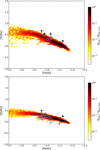 |
Fig. C.1 [O/Fe] (top panel) and [Si/Fe] (bottom panel) abundances as a function of [Fe/H] as predicted by our adopted stochastic chemical evolution model. The colormap displays the number of predicted long-lived stars by the model on a logarithmic scale. Black symbols are as in Fig. 12. |
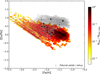 |
Fig. C.2 [Eu/Fe] abundances as a function of [Fe/H] as predicted by our adopted stochastic chemical evolution model with a reduced fraction of systems originating NSM. The colormap displays the number of predicted long-lived stars by the model on a logarithmic scale. As a comparison, we plot in grayscale the result by the stochastic chemical evolution model using our fiducial setup. Black symbols are as in Fig. 12. |
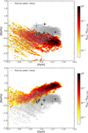 |
Fig. C.3 [Ba/Fe] abundances as a function of [Fe/H] as predicted by our adopted stochastic chemical evolution model with a reduced fraction of systems originating NSM (top panel) and rotational velocity distribution for massive stars favouring higher velocities (bottom panel). The colormap displays the number of predicted long-lived stars by the model on a logarithmic scale. As a comparison, we plot in grayscale the result by the stochastic chemical evolution model using our fiducial setup. Black symbols are as in Fig. 12. |
All Tables
All Figures
|
Fig. 1 Comparison between UVES-3 and MIKE-2 spectra after reduction, normalisation, radial velocity, and heliocentric corrections. The two stars share similar atmospheric parameters and iron abundances. Black ticks mark the position of observable lines. |
| In the text | |
|
Fig. 2 Upper panel: theoretical AMR of the SMC (black line, Pagel & Tautvaisiene 1998), superimposed with the SMC GCs (Paper II, green circles). The white dots mark the position on the theoretical AMR of ages 11, 12 and 13 Gyr. Lower panel: average Si and Ca abundances as a function of [Fe/H] for SMC stars of this work observed with UVES (red squares) and MIKE (red triangles). The blue shaded area highlights the [Fe/H] region of the stars of our sample with −2.2 < [Fe/H] < −1.8 dex. |
| In the text | |
|
Fig. 3 α-elements patterns: [O/Fe], [Mg/Fe], [Si/Fe], and [Ca/Fe] abundances as a function of [Fe/H] for SMC stars of this work observed with UVES (red squares) and MIKE (red triangles), together with the SMC field stars (Paper I, red small circles) and the SMC GCs (Paper II, green circles). Error bars are shown for UVES and MIKE abundances. As a reference, Gaussian KDE regressions of MW abundances built from SAGA database (Suda et al. 2008) (blue line) are reported, together with their 1σ confidence interval (blue shaded area), in the background. |
| In the text | |
|
Fig. 4 [Eu/Fe] abundances as a function of [Fe/H]. Same symbols as in Fig. 3, but the red small circles are SMC field stars observed with GIRAFFE from Paper IV. |
| In the text | |
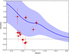 |
Fig. 5 [Sm/Fe] abundances as a function of [Fe/H]. Same symbols as in Fig. 3. |
| In the text | |
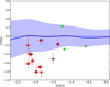 |
Fig. 6 [Y/Fe] abundances as a function of [Fe/H]. Same symbols as in Fig. 3. |
| In the text | |
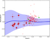 |
Fig. 7 [Ba/Fe] abundances as a function of [Fe/H]. Same symbols as in Fig. 3. |
| In the text | |
 |
Fig. 8 [La/Fe] abundances as a function of [Fe/H]. Same symbols as in Fig. 3. |
| In the text | |
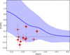 |
Fig. 9 [Ce/Fe] abundances as a function of [Fe/H]. Same symbols as in Fig. 3. |
| In the text | |
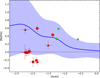 |
Fig. 10 [Nd/Fe] abundances as a function of [Fe/H]. Same symbols as in Fig. 3. |
| In the text | |
|
Fig. 11 [Y/Eu], [Ba/Eu], [La/Eu], [Ce/Eu], [Nd/Eu] and [Sm/Eu] abundances as a function of [Fe/H] for SMC stars observed with UVES (squares) and MIKE (triangles). Points are coloured according to their [Eu/Fe] abundances. Lower limits are reported with arrows. In each plot, the linear regression of the measured abundances and their 95% confidence intervals are shown with a green dashed line and green shaded area, respectively. |
| In the text | |
|
Fig. 12 [Eu/Fe] abundances as a function of [Fe/H] as predicted by our adopted stochastic chemical evolution model. The colormap displays the number density of predicted long-lived stars by the model on a logarithmic scale. Observed SMC abundances with relative errorbar are represented with black symbols (squares: UVES observations, triangles: MIKE observations). |
| In the text | |
|
Fig. 13 [Ba/Fe] abundances as a function of [Fe/H] as predicted by our adopted stochastic chemical evolution model. On the left panel, the colormap displays the number density of predicted long-lived stars by the model on a logarithmic scale. On the right panel, the colormap displays the fraction of element abundance produced by s-process over total. Black symbols are as in Fig. 12. |
| In the text | |
|
Fig. C.1 [O/Fe] (top panel) and [Si/Fe] (bottom panel) abundances as a function of [Fe/H] as predicted by our adopted stochastic chemical evolution model. The colormap displays the number of predicted long-lived stars by the model on a logarithmic scale. Black symbols are as in Fig. 12. |
| In the text | |
|
Fig. C.2 [Eu/Fe] abundances as a function of [Fe/H] as predicted by our adopted stochastic chemical evolution model with a reduced fraction of systems originating NSM. The colormap displays the number of predicted long-lived stars by the model on a logarithmic scale. As a comparison, we plot in grayscale the result by the stochastic chemical evolution model using our fiducial setup. Black symbols are as in Fig. 12. |
| In the text | |
|
Fig. C.3 [Ba/Fe] abundances as a function of [Fe/H] as predicted by our adopted stochastic chemical evolution model with a reduced fraction of systems originating NSM (top panel) and rotational velocity distribution for massive stars favouring higher velocities (bottom panel). The colormap displays the number of predicted long-lived stars by the model on a logarithmic scale. As a comparison, we plot in grayscale the result by the stochastic chemical evolution model using our fiducial setup. Black symbols are as in Fig. 12. |
| In the text | |
Current usage metrics show cumulative count of Article Views (full-text article views including HTML views, PDF and ePub downloads, according to the available data) and Abstracts Views on Vision4Press platform.
Data correspond to usage on the plateform after 2015. The current usage metrics is available 48-96 hours after online publication and is updated daily on week days.
Initial download of the metrics may take a while.