| Issue |
A&A
Volume 706, February 2026
|
|
|---|---|---|
| Article Number | A67 | |
| Number of page(s) | 14 | |
| Section | Planets, planetary systems, and small bodies | |
| DOI | https://doi.org/10.1051/0004-6361/202558040 | |
| Published online | 03 February 2026 | |
Coexistence of coagulation and streaming instabilities in protoplanetary disks
1
Laboratoire d’astrophysique de Bordeaux, Univ. Bordeaux, CNRS, B18N, allée Geoffroy Saint-Hilaire,
33615
Pessac,
France
2
Institute of Astronomy and Astrophysics, Academia Sinica,
Taipei
10617,
Taiwan
3
Physics Division, National Center for Theoretical Sciences,
Taipei City
10617,
Taiwan
★ Corresponding author: This email address is being protected from spambots. You need JavaScript enabled to view it.
Received:
9
November
2025
Accepted:
12
December
2025
Abstract
The streaming instability is considered to be one of the leading candidates for the formation of planetesimals, given its ability to overcome the bouncing and fragmentation barriers. However, the formation of dense dust clumps through this process is possible provided it involves solids with dimensionless stopping times ~0.1 in standard disks, which typically corresponds to 1–10 cm-sized particles. This implies that dust coagulation is required for the SI to be an efficient process. Here, we employ unstratified, shearing-box simulations combined with a moment equation for solving the coagulation equation to examine the effect of dust growth on the SI. In dust-rich disks with a dust-to-gas ratio ϵ ≳ 1, coagulation is found to have little impact on the SI. Meanwhile, in dust-poor disks with ϵ ~ 0.01, we observe the formation of vertically extended filaments through the action of the coagulation instability (CI), which is triggered due to the dependence of coagulation efficiency on dust density. For moderate dust-to-gas ratios ϵ ~ 0.1 and Stokes numbers St ≲ 0.1, we find an onset of the SI within these filaments, with a linear growth rate significantly higher compared to standard SI. We refer to this regime as coagulation-assisted SI. The synergy between both instabilities in that case leads to isotropic turbulence and dust concentrations that are increased by a factor of 30–40. As dust continues to grow, SI tends to overcome the effect of the CI such that the nonlinear saturation phase is similar to pure SI. Our results suggest that coagulation, by simply increasing dust size, could facilitate the formation of dense clumps through the SI, although we note that it has only a slight effect on its nonlinear evolution.
Key words: hydrodynamics / instabilities / methods: analytical / methods: numerical / planets and satellites: formation
© The Authors 2026
 Open Access article, published by EDP Sciences, under the terms of the Creative Commons Attribution License (https://creativecommons.org/licenses/by/4.0), which permits unrestricted use, distribution, and reproduction in any medium, provided the original work is properly cited.
This article is published in open access under the Subscribe to Open model. This email address is being protected from spambots. You need JavaScript enabled to view it. to support open access publication.
1 Introduction
In the standard scenario for planet formation, the coagulation of micron-sized grains leads to the formation of millimeter-sized dust (Dullemond & Dominik 2005). However, any further growth of particles above the millimeter-size range is rendered difficult because of bouncing (Zsom et al. 2010) and fragmentation (Zsom et al. 2010) barriers. An emerging scenario that is capable of overcoming these barriers is based on the assumption that 100-km sized planetesimals form directly through the streaming instability (SI; Youdin & Goodman 2005; Youdin & Johansen 2007), which occurs as a result of angular momentum exchange between the gas and dust components, as well as rotation. It has been shown that during the nonlinear evolution of the SI, dust particles can eventually directly concentrate into clumps or filaments, which can subsequently become gravitationally unstable to form 100–1000 km-sized bodies (Johansen et al. 2009; Simon et al. 2016; Abod et al. 2019). The ability for solids to experience a regime of strong clumping depends mainly on the dimensionless stopping time St and local dust-to-gas ratio, ϵ, which can also be quantified through the dust-to-gas surface density ratio, Z = Σd/Σg, where Σd (resp. Σg) is the dust (resp. gas) surface density. For Z ~ 5 × 10⁻³, strong clumping requires St ≳ 0.1 in a disk where no external turbulence operates, whereas for St ≲ 0.01 strong clumping is triggered for a critical solid abundance of a few percent (Carrera et al. 2015; Yang et al. 2017; Li & Youdin 2021). In any case, this suggests that a level of dust growth is needed for the SI to enter the strong clumping regime (Drążkowska & Dullemond 2014).
Nonetheless, taking into account the effect of dust growth on the SI in a self-consistent fashion is a difficult task. The process of dust growth is indeed expected to be a sensitive function of the relative collision velocity between grains, which depends on multiple processes taking place in the protoplanetary disk. As a consequence, the resulting dust size distribution is not known a priori and remains uncertain. The generalization of the classical, monodisperse SI to multiple dust sizes has been examined by a number of recent studies, but on the basis of prescribed dust size distributions. These have shown that the growth rate of the polydisperse, multispecies SI (PSI) tends to decrease as the number of species is increased (Krapp et al. 2019) and becomes very small in the limit of a continuous size distribution (Paardekooper et al. 2020; Zhu & Yang 2021). However, it was also found that a top-heavy size distribution, resulting for instance from a pure coagulation process, leads to PSI linear growth rates equivalent to those of the classical SI (McNally et al. 2021).
The influence of the process of coagulation itself on the nonlinear development of the monodisperse SI has been investigated by Ho et al. (2024) using stratified simulations. These authors found that coagulation tends to broaden the range of Stokes numbers and dust-to-gas ratios over which the SI can be triggered, due to ability for coagulation to promote dust growth. Conversely, it has even been proposed that dust growth can be significantly boosted in the strong clumping regime of the SI (Tominaga & Tanaka 2023, 2025). This arises because dust-loading increases the inertia of the dusty fluid, resulting in a reduction of the effective sound speed and lower collision velocities between dust grains. These results suggest that a feedback loop between coagulation and the development of the SI may exist and this was recently studied by Carrera et al. (2025).
In this paper, we examine the effect of the coagulation instability (CI) on the linear growth and nonlinear saturation phase of the SI (Tominaga et al. 2021). The CI is a consequence of the interplay between the dust coagulation process and radial drift of dust particles and primarily related to the dependence of mass growth rate on dust density. As described by Tominaga et al. (2021), if we assume a positive dust density perturbation, the resulting increased coagulation efficiency leads to a variation of the dust size. This subsequently causes an enhanced radial drift speed which tends to amplify the initial density perturbation, resulting in a feedback loop. It has been shown that the nonlinear evolution of the CI can enable the Stokes number of solids to rapidly reach unity, even for relatively modest dust-to-gas ratios ϵ ~ 10−3 (Tominaga et al. 2022a,b). Therefore, the CI might represent a promising mechanism to extend the parameter space (in terms of dust-to-gas ratios and Stokes numbers) over which the SI can operate efficiently.
To investigate the possible effect of the CI on the SI in more detail, we performed 2D axisymmetric, unstratified, shearingbox simulations in which coagulation was modeled using the single-size approximation. Our main aims are to (i) assess whether the CI can help the SI enter the regime of strong clumping and (ii) evaluate to what extent the turbulence driven by the CI subsequently impacts the nonlinear development of the SI.
The paper is organized as follows. In Sect. 2, we present the governing evolution equations of the gas and dust components. We then describe in Sect. 3 the numerical setup and the initial conditions that are used in the simulations, whose results are presented in Sect. 4. We discuss our results in Sect. 5 and present a summary of our findings in Sect. 6.
2 Physical model
2.1 Governing equations
We modeled a local patch in a protoplanetary disk within the shearing box framework. A Cartesian coordinate system with origin located at an arbitrary distance, R0, from the central star corotates with angular velocity Ω0 = Ωk(R0), with Ωk representing the Keplerian angular velocity. The x- and y-axes are oriented radially outward and along the orbital direction respectively, while the z-axis is directed in the vertical direction. We assume that the domain is small compared to the orbital distance so that Keplerian rotation appears as a linear shear flow with velocity ![Mathematical equation: $\[\mathbf{U}_{\mathbf{k}}=-\frac{3}{2} x \Omega_{0} \hat{\mathbf{y}}\]$](/articles/aa/full_html/2026/02/aa58040-25/aa58040-25-eq1.png) . We assumed the system is axisymmetric and neglect the vertical component of stellar gravity. In these limits, the continuity and momentum equations for the gas and dust components are, respectively, given by
. We assumed the system is axisymmetric and neglect the vertical component of stellar gravity. In these limits, the continuity and momentum equations for the gas and dust components are, respectively, given by
![Mathematical equation: $\[\frac{\partial \rho_g}{\partial t}+\nabla \cdot\left(\rho_g \mathbf{u}\right)=0,\]$](/articles/aa/full_html/2026/02/aa58040-25/aa58040-25-eq2.png) (1)
(1)
![Mathematical equation: $\[\begin{aligned}\frac{\partial \mathbf{u}}{\partial t}+\mathbf{u} \cdot \nabla \mathbf{u}= & 2 u_y \Omega \hat{\mathbf{x}}-u_x \frac{\Omega}{2} \hat{\mathbf{y}}-\frac{1}{\rho_g} \nabla P+2 \eta R \Omega^2 \hat{\mathbf{x}}+\frac{\epsilon}{\tau_s}(\mathbf{v}-\mathbf{u}) \\& +\frac{1}{\rho_g} \nabla \cdot \mathbf{T}\end{aligned}\]$](/articles/aa/full_html/2026/02/aa58040-25/aa58040-25-eq3.png) (2)
(2)
![Mathematical equation: $\[\frac{\partial \rho_d}{\partial t}+\nabla \cdot\left(\rho_d \mathbf{v}\right)=\nabla \cdot\left(D \rho_d \nabla \epsilon\right),\]$](/articles/aa/full_html/2026/02/aa58040-25/aa58040-25-eq4.png) (3)
(3)
![Mathematical equation: $\[\frac{\partial \mathbf{v}}{\partial t}+\mathbf{v} \cdot \nabla \mathbf{v}=2 v_y \Omega \hat{\mathbf{x}}-v_x \frac{\Omega}{2} \hat{\mathbf{y}}-\frac{1}{\tau_s}(\mathbf{v}-\mathbf{u}),\]$](/articles/aa/full_html/2026/02/aa58040-25/aa58040-25-eq5.png) (4)
(4)
where ρg and ρd are the gas and dust densities, respectively, and u, v are their velocities measured in relation to the background Keplerian shear. We adopted an isothermal equation of state, ![Mathematical equation: $\[P= \rho_{g} c_{s}^{2}\]$](/articles/aa/full_html/2026/02/aa58040-25/aa58040-25-eq6.png) , where cs = HgΩ0 is the (constant) sound speed, with Hg as the gas pressure scale height. In Eq. (2), T is the viscous stress tensor, given by
, where cs = HgΩ0 is the (constant) sound speed, with Hg as the gas pressure scale height. In Eq. (2), T is the viscous stress tensor, given by
![Mathematical equation: $\[\mathbf{T}=\rho_g \nu\left(\nabla \mathbf{u}+(\nabla \mathbf{u})^{\dagger}-\frac{2}{3} I ~\nabla \cdot \mathbf{u}\right),\]$](/articles/aa/full_html/2026/02/aa58040-25/aa58040-25-eq7.png) (5)
(5)
where ν is the kinematic viscosity employed to model the effects of possible underlying turbulence. Regarding the resulting turbulence-induced particle stirring, it is modeled by the source term appearing in the dust continuity equation, where D is the dust diffusion coefficient that is set here to D = ν. It is important to note that viscosity and diffusion are generally not included in our simulations, except in those presented in Appendix B.
In Eq. (2), the term ∝ η corresponds to an outward force acting on the gas due to a background radial pressure gradient, and determined by the dimensionless parameter,
![Mathematical equation: $\[\eta=-\frac{1}{2 \rho_g \Omega_0^2 R_0} \frac{\partial P}{\partial r}.\]$](/articles/aa/full_html/2026/02/aa58040-25/aa58040-25-eq8.png) (6)
(6)
Finally, τs is the stopping time that we will characterize in the following in terms of the dimensionless Stokes number, St = τs Ω. Dust grains are assumed to be in the Epstein regime such that St is the related to the grain size, a, via
![Mathematical equation: $\[\mathrm{St}=\sqrt{\frac{\pi}{8}} \frac{\rho_i a}{\rho_g c_s} \Omega,\]$](/articles/aa/full_html/2026/02/aa58040-25/aa58040-25-eq9.png) (7)
(7)
where ρi is the internal density of dust grains, and m =4πρia3/3 their mass. In this work, we allowed m (and consequently a) to increase as a result of dust coagulation, which we modeled using a single-size approximation (Sato et al. 2016; Tominaga et al. 2021). This consists of following the size evolution of grains whose mass, mp, dominate the dust density distribution at each location. The evolution equation for the so-called peak mass, mp, can be obtained by considering the first-moment of the Smoluchowski equation (e.g., Appendix A of Tominaga et al. 2021), expressed as
![Mathematical equation: $\[\frac{\partial m_p}{\partial t}+\mathbf{v} \cdot \nabla\left(m_p\right)=\mathcal{S}^{+}\left(\mathrm{St}_p\right)-\mathcal{S}^{-},\]$](/articles/aa/full_html/2026/02/aa58040-25/aa58040-25-eq10.png) (8)
(8)
where ![Mathematical equation: $\[\mathcal{S}^{+}=4 \pi a_{p}^{2} \Delta v_{\mathrm{pp}} \rho_{d}\]$](/articles/aa/full_html/2026/02/aa58040-25/aa58040-25-eq11.png) , with ap the grain size corresponding to mp and Δvpp the typical relative velocity between particles, is the mass growth rate resulting from coagulation. This value can generally be expressed as a function of the Stokes number Stp corresponding to mp. Although dissipation effects were not included in our dynamical equations, we followed Tominaga et al. (2021) and assumed that relative velocities are dominated by the turbulence experienced by the disk. This allowed us to i) make the problem analytically tractable and ii) identify clearly the role played by coagulation. In that case and within the limit St << 1, we can further make use of a simplified expression for Δvpp given by (Ormel & Cuzzi 2007):
, with ap the grain size corresponding to mp and Δvpp the typical relative velocity between particles, is the mass growth rate resulting from coagulation. This value can generally be expressed as a function of the Stokes number Stp corresponding to mp. Although dissipation effects were not included in our dynamical equations, we followed Tominaga et al. (2021) and assumed that relative velocities are dominated by the turbulence experienced by the disk. This allowed us to i) make the problem analytically tractable and ii) identify clearly the role played by coagulation. In that case and within the limit St << 1, we can further make use of a simplified expression for Δvpp given by (Ormel & Cuzzi 2007):
![Mathematical equation: $\[\Delta v_{\mathrm{pp}}=\sqrt{C \mathrm{St}_p \alpha_{\mathrm{coag}}} c_s.\]$](/articles/aa/full_html/2026/02/aa58040-25/aa58040-25-eq12.png) (9)
(9)
Here, C is a numerical factor set to C = 2.3 and α is the dimensionless turbulent stress parameter (Shakura & Sunyaev 1973), which we fixed to αcoag = 10−4. In the following and for convenience, we simply drop the subscript p in the definition of Stp and ap so that (unless otherwise stated) we have ![Mathematical equation: $\[\mathrm{St}=\sqrt{\frac{\pi}{8}} \frac{\rho_{i} a}{\rho_{g} c_{s}} \Omega\]$](/articles/aa/full_html/2026/02/aa58040-25/aa58040-25-eq13.png) with ρi = 3mp/4πa3.
with ρi = 3mp/4πa3.
With respect to the original work of Tominaga et al. (2021), we included in the mass evolution equation (Eq. (8)) an additional, constant sink term, 𝒮−, whose value was set to the initial value of 𝒮+. The primary aim of adding this term is to ensure that the initial chosen particle mass corresponds to an equilibrium solution to the set of Eqs. (1)–(4), combined with Eq. (8). Given the radial and vertical dependences of equilibrium quantities are ignored in the box, the left-hand side of Eq. (8) becomes zero at steady-state, thereby leading to 𝒮− = 𝒮+.
We notice that in principle, dust loading leads to a reduction of the sound speed by increasing the inertia of the dusty fluid. This can be expressed by defining an effective sound speed given by (Lin & Youdin 2017):
![Mathematical equation: $\[\tilde{c}_s=\frac{c_s}{\sqrt{1+\epsilon}}.\]$](/articles/aa/full_html/2026/02/aa58040-25/aa58040-25-eq14.png) (10)
(10)
From Eq. (9), we see a reduction in the sound speed due to dust-loading results in a decrease in the collision velocity. Recent works have shown that this effect may cause rapid dust growth in the strong clumping regime of the SI, due to the significant increase in the local dust-to-gas ratio there (Tominaga & Tanaka 2023, 2025; Carrera et al. 2025). Here, we do not account for this potential important effect and simply employ the nominal sound speed when computing the collision velocity.
2.2 Equilibrium state
For constant values of ρg, ρd, and St, equilibrium solutions to Eqs. (1)–(4) can be obtained, leading to velocity deviations from Keplerian rotation given by
![Mathematical equation: $\[u_x=\frac{2 \epsilon \mathrm{St}}{\Delta^2} \eta R_0 \Omega,\]$](/articles/aa/full_html/2026/02/aa58040-25/aa58040-25-eq15.png) (11)
(11)
![Mathematical equation: $\[u_y=-\frac{\left(1+\epsilon+\mathrm{St}^2\right)}{\Delta^2} \eta R_0 \Omega,\]$](/articles/aa/full_html/2026/02/aa58040-25/aa58040-25-eq16.png) (12)
(12)
![Mathematical equation: $\[v_x=\frac{-2 \mathrm{St}}{\Delta^2} \eta R_0 \Omega,\]$](/articles/aa/full_html/2026/02/aa58040-25/aa58040-25-eq17.png) (13)
(13)
![Mathematical equation: $\[v_y=-\frac{(1+\epsilon)}{\Delta^2} \eta R_0 \Omega,\]$](/articles/aa/full_html/2026/02/aa58040-25/aa58040-25-eq18.png) (14)
(14)
where Δ2 = St2 + (1 + ϵ)2. For a fixed grain size, these solutions correspond to the traditional steady-state drift solutions for a dusty disk obtained by Nakagawa et al. (1986). As mentioned above, the inclusion of coagulation would not be expected to impact these equilibrium solutions given the presence of the sink term in the right-hand side of Eq. (8).
3 Methodology
3.1 Numerical method and model setup
We examined the nonlinear dynamical evolution of the system by performing 2.5D (axisymmetric), unstratified simulations in a shearing-box using the multifluid version of the publicly available code FARGO3D (Benítez-Llambay & Masset 2016; Benítez-Llambay et al. 2019). We considered single dust species runs in which the effect of coagulation was implemented in the aforementioned single-size approximation, albeit using a conservative version of Eq. (8), expressed as
![Mathematical equation: $\[\frac{\partial m_p \rho_d}{\partial t}+\nabla \cdot\left(m_p \rho_d \mathbf{v}\right)=p_{\mathrm{eff}}\left(\mathcal{S}^{+}-\mathcal{S}^{-}\right) \rho_d.\]$](/articles/aa/full_html/2026/02/aa58040-25/aa58040-25-eq19.png) (15)
(15)
Using this form, the previous equation can be integrated using the operator splitting technique employed by FARGO3D, with a coagulation term solved as a new substep within the source step. Tests of the implementation are presented in Appendix A. With respect to Eq. (8), the previous expression includes an additional, sticking efficiency, term peff whose expression is similar to that used by Tominaga et al. (2022a):
![Mathematical equation: $\[p_{\mathrm{eff}}=\min \left(1,-\frac{\ln \left(\mathrm{St} / \mathrm{St}_f\right)}{\ln 5}\right),\]$](/articles/aa/full_html/2026/02/aa58040-25/aa58040-25-eq20.png) (16)
(16)
which also prevents the value of the Stokes number from increasing above Stf. This enables us to (i) take into account the effect of the fragmentation process in the simulations and (ii) examine the evolution outcome as a function of parameter Stf.
In our shearing-box setup, the Cartesian coordinate system is oriented with x along the (outward) radial direction and z pointing along the (upward) vertical direction. The domain considered is such that x ∈ [−0.0125, 0.0125] and z ∈ [−0.0025, 0.0025] or, equivalently, x ∈ (−0.25, 0.25)H0 and z ∈ (−0.05, 0.05)H0. The appropriate size of the shearing-box was determined from convergence tests; however, typically, a large radial extent of the domain is needed to accommodate the most unstable wavelength expected from linear growth maps of the SI as St → Stf, whereas the small vertical extent of the domain is consistent with an unstratified setup, focusing on the disk midplane. The domain is covered by Nx × Nz = 2048 × 512 grid cells, with the radial resolution chosen specifically to capture the largest number of CI unstable modes, as these have growth rates increasing with the radial wavenumber in the absence of diffusive processes. As we do not consider the vertical gravity in this work, boundaries are taken to be periodic in the z-direction, while we use standard shearing periodic boundaries in x.
3.2 Parameters and initial conditions
We adopted a unique value for the pressure gradient parameter, η = 0.005, corresponding to a typical pressure gradient in a protoplanetary disk. Three values for the initial dust-to-gas mass ratio, ϵ, were considered, ϵ = 0.02, 0.2, 3, which are representative of low (ϵ = 0.02), moderate (ϵ = 0.2), and high dust abundances (ϵ = 3). For simulations where dust coagulation was discarded, the Stokes number was kept constant with values: St = 0.01, 0.1, 1; whereas in those including coagulation, the Stokes number was computed from Eq. (15), starting from an initial value of Sti = 10−3. The details of parameters for each simulation are presented in Table 1.
Regarding the initial conditions, radial and azimuthal components of dust and gas velocities were initialized according to Eqs. (11)–(14), while setting the vertical component to zero. In most runs, the initial dust velocities were then seeded with random noise of amplitude 10−2cs. Because the effects of stratification were not considered, we used an initial gas density of ρ0 = 1. We also used a system of units where cs = Ωk = Hg = 1.
Summary of the parameters adopted in our runs.
3.3 Diagnostics
One aim of this work is to assess the level of turbulence generated by the coagulation and streaming instabilities. To quantify the flux of angular momentum carried by turbulence, we first define the Shakura–Sunyaev stress parameter (Shakura & Sunyaev 1973):
![Mathematical equation: $\[<\alpha_{\mathrm{SS}}>=\frac{<\rho_g u_x u_y>}{\rho_0 c_s^2},\]$](/articles/aa/full_html/2026/02/aa58040-25/aa58040-25-eq21.png) (17)
(17)
where the symbol <> denotes averaging in the x–z plane. To obtain a reliable measure of αSS, we further performed a time average of the latter quantity, expressed as
![Mathematical equation: $\[\overline{<\alpha_{\mathrm{SS}}>}=\frac{1}{t_2-t_1} \int_{t_1}^{t_2}<\alpha_{\mathrm{SS}}>d t,\]$](/articles/aa/full_html/2026/02/aa58040-25/aa58040-25-eq22.png) (18)
(18)
which we typically compute over a time interval of Δt = t2 − t1 ~ 10Ω−1 once saturation has been attained. We also measured the velocity dispersion of the gas δu whose ith component as
![Mathematical equation: $\[\delta u_i=\sqrt{<u_i^2>-<u_i>^2},\]$](/articles/aa/full_html/2026/02/aa58040-25/aa58040-25-eq23.png) (19)
(19)
along with the autocorrelation time, tc,i, of the velocity fluctuations, obtained by evaluating each component of the autocorrelation function given by (Yang et al. 2018):
![Mathematical equation: $\[\mathcal{R}_i(t)=\int\left[u_i(\tau)-\overline{u_i}\right]\left[u_i(t+\tau)-\overline{u_i}\right] d \tau.\]$](/articles/aa/full_html/2026/02/aa58040-25/aa58040-25-eq24.png) (20)
(20)
In the previous expression, ![Mathematical equation: $\[\bar{u}\]$](/articles/aa/full_html/2026/02/aa58040-25/aa58040-25-eq25.png) is the mean velocity, whose components ui are estimated by considering their time average in the interval [t1, t2],
is the mean velocity, whose components ui are estimated by considering their time average in the interval [t1, t2],
![Mathematical equation: $\[\overline{u_i}=\frac{1}{t_2-t_1} \int_{t_1}^{t_2} u_i(\tau) d \tau.\]$](/articles/aa/full_html/2026/02/aa58040-25/aa58040-25-eq26.png) (21)
(21)
Following Hsu & Lin (2022), we set t2 − t1 = 5P and recorded the data with a cadence of 0.01P (Yang et al. 2018) to compute Eq. (20). We then determined tc,i by fitting an exponential function to the autocorrelation function (Fromang & Papaloizou 2006).
From Eqs. (19) and (20), we can subsequently compute the gas bulk diffusion coefficient, Dg,i, in the ith direction, expressed as
![Mathematical equation: $\[D_{g, i}={\overline{\delta u_i}}^2 t_{c, i}.\]$](/articles/aa/full_html/2026/02/aa58040-25/aa58040-25-eq27.png) (22)
(22)
In the following, we made use of the dimensionless bulk gas diffusion coefficient instead, defined by
![Mathematical equation: $\[\alpha_{g, i}=\frac{D_{g, i}}{c_s H_g}=\left(\frac{\overline{\delta u_i}}{c_s}\right)^2 \tau_{c, i},\]$](/articles/aa/full_html/2026/02/aa58040-25/aa58040-25-eq28.png) (23)
(23)
where τc,i is the dimensionless equivalent of the correlation time,
![Mathematical equation: $\[\tau_{c, i}=t_{c, i} \Omega_0^{-1}.\]$](/articles/aa/full_html/2026/02/aa58040-25/aa58040-25-eq29.png) (24)
(24)
4 Results
In this section, we discuss the impact of dust coagulation on the nonlinear evolution of the SI by providing a systematic comparison between pure SI simulations and runs that include dust coagulation. Our comparisons rely on models in which the maximum Stokes number Stf coincides with the value for St set in standard SI simulations. For simplicity, we chose to simply denote Stf as St when presenting the results of the simulations.
In Fig. 1, we present an overview of the results, where we show the time evolution of the maximum dust-to-gas ratio, ϵmax, and Stokes number, St, for each model we considered. From this figure, it is immediately obvious that in dust rich disks, the impact of coagulation is relatively weak as simulations that include this effect reach overdensities that are very similar to those obtained in standard SI simulations.
In dust-poor disks with ϵ < 0.2, however, including coagulation has a stronger effect, with overdensities that can be a factor of 5–30 higher than without coagulation for tightly coupled particles. In this regime, we find that the CI (Tominaga et al. 2021) plays an important role in the evolution, as it is found to dominate over other processes for ϵ = 0.02, or even interact with the SI for ϵ = 0.2. Below, we describe these two different modes of evolution found for Stokes numbers St < 0.1 in more details. We then discuss the case of marginally coupled particles with St ≈ 1.
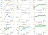 |
Fig. 1 Time evolution of the maximum dust-to-gas ratio, ϵmax, and Stokes number for all simulations listed in Table 1. The left, middle, and right columns correspond to ϵ = 0.02, 0.2, 3, respectively, while the upper, middle, and lower panels correspond to St = 0.01, 0.1, 1 respectively. In each panel, we show the evolution of ϵmax for the case with (blue) and without (green) coagulation. For the evolution of St, the light colour traces the minimum and maximum values, whereas the dark colour traces the box averaged value. |
4.1 Tightly coupled particles
4.1.1 ϵ = 0.02: Evolution mediated by Cl
The CI is by essence a dust-driven instability which involves two ingredients: (i) the dust-density density dependence of the collisional coagulation rate and (ii) the dependence of St with the particle size. When these are mixed, a dust surface density perturbation δΣd leads to a radial variation of St, resulting in a traffic jam which tends to enhance δΣd. Compared to other dust-driven instabilities, the CI can develop over a few orbital periods even for small dust-to-gas ratios ϵ ~ 10−3. More precisely, the growth rate of the CI is typically given by (Tominaga et al. 2021):
![Mathematical equation: $\[\left.\sigma=\sqrt{\left.\frac{1}{2} \frac{\epsilon}{3 t_0} k \right\rvert\,<v_x>} \right\rvert\, \Omega^{-1},\]$](/articles/aa/full_html/2026/02/aa58040-25/aa58040-25-eq30.png) (25)
(25)
where k is the radial wavenumber and vx is given by Eq. (13). Then, ![Mathematical equation: $\[t_{0}=4 / 3 \sqrt{2 \mathrm{St}_{i} / \alpha C \pi}\]$](/articles/aa/full_html/2026/02/aa58040-25/aa58040-25-eq31.png) is the mass growth timescale of a dust particle and can be obtained from Eq. (8). For Sti = 10−3 and ϵ = 0.02, setting kH = 4 × 10³, which corresponds to the maximum wavenumber that is resolved by ≈6 grid cells, we get σ ≈ 2.10−3Ω−1. The time evolution of the maximum dust-to-gas ratio and Stokes number is shown, for ϵ = 0.02 and St = 0.01 (Model E0v02S0v01c), in the upper-left panel of Fig. 1. Both quantities exhibit an initial rapid exponential growh phase and then reach nonlinear saturation at t ~ 1500Ω−1. We note in passing that in the context of the CI, unstable modes are essentially incompressible such that the evolution of ϵmax reflects the evolution of the maximum of the perturbed dust density, δρd. From this plot, we can estimate a linear growth rate of σ ~ 1.7 × 10⁻³Ω−1 during the initial linear growth phase, which is in good agreement with our previous analytical estimation. This clearly indicates that the CI is responsible for the initial increase in δρd and St that are observed, although disentangling the effect of the CI from the evolution of the averaged Stokes number is more difficult. For such small values of ϵ and St, we also note that the effect of the SI is expected to be negligible. This can be confirmed by inspecting the evolution for the case where coagulation is switched off (green line) and for which ϵmax remains close to its initial value.
is the mass growth timescale of a dust particle and can be obtained from Eq. (8). For Sti = 10−3 and ϵ = 0.02, setting kH = 4 × 10³, which corresponds to the maximum wavenumber that is resolved by ≈6 grid cells, we get σ ≈ 2.10−3Ω−1. The time evolution of the maximum dust-to-gas ratio and Stokes number is shown, for ϵ = 0.02 and St = 0.01 (Model E0v02S0v01c), in the upper-left panel of Fig. 1. Both quantities exhibit an initial rapid exponential growh phase and then reach nonlinear saturation at t ~ 1500Ω−1. We note in passing that in the context of the CI, unstable modes are essentially incompressible such that the evolution of ϵmax reflects the evolution of the maximum of the perturbed dust density, δρd. From this plot, we can estimate a linear growth rate of σ ~ 1.7 × 10⁻³Ω−1 during the initial linear growth phase, which is in good agreement with our previous analytical estimation. This clearly indicates that the CI is responsible for the initial increase in δρd and St that are observed, although disentangling the effect of the CI from the evolution of the averaged Stokes number is more difficult. For such small values of ϵ and St, we also note that the effect of the SI is expected to be negligible. This can be confirmed by inspecting the evolution for the case where coagulation is switched off (green line) and for which ϵmax remains close to its initial value.
Figure 2 shows snapshots of the dust density and Stokes number at saturation, for this model and in the case with ϵ = 0.02 and St = 0.1 (Model E0v02S0v01c) for which a similar mode of evolution is found. Since the CI is originally a one-dimensional instability with no dependence in the vertical direction, it is not surprising to observe the formation of vertically extended filaments, whose number tends to decrease as St is increased. For St = 0.1, we indeed ultimately obtain a single filament with ϵmax ≈ 0.1; whereas for St = 0.01, five filaments remain in the system at the end of the simulation with consequently smaller ϵmax ≈ 0.006. We find that these filaments are themselves formed through the merging of thinner ones. This is illustrated in Fig. 3, where we display the vertically averaged dust density as a function of time and radial position. From this figure, it is clear that filaments grow not only via merging events but also by simply collecting dust as they drift inward. Both effects then combine to make the amplitude of the perturbed dust density start level off and saturate at later times. Another mechanism that may contribute to saturation is the level of turbulence generated by the CI itself. This is suggested by looking back to Fig. 2, where it is evident that turbulence operates in the disk, especially for St = 0.1. In this case, the time evolution of the dimensionless bulk gas diffusion coefficients, αg,i, is shown in the upper panel of Fig. 4. Not surprisingly, this reveals anisotropy of the CI with an enhanced dust diffusion coefficient αg,z of 𝒪(10−6) in the vertical direction, which is larger by two orders of magnitude compared to αg,y. A similar trend is also found for St = 0.01 (see Table 1), with αg,z of 𝒪(10−7) and αg,y of 𝒪(10−8) in that case. The bottom panel of Fig. 4 compares linear growth rates for αg,i = 0 (left) and for αg,i = 3 × 10⁻⁶ (right), and which have been obtained from the linearized equations presented in Appendix A using ν = D = αg,icsHg. We see that the turbulent diffusion induced by the CI itself can indeed significantly cut off the most unstable modes corresponding to αg,i = 0. Although it is not shown here, we found a similar effect for St = 0.01, which confirms that the CI-induced dust diffusion can also contribute to the saturation of the instability.
In summary, we find that for tightly coupled particles, the CI can operate in dust-poor disks and lead to the formation of dust rings with ϵmax of 𝒪(0.1). However, this is not enough to subsequently trigger the SI within these rings because the dust backreaction onto the gas tends to significantly regulate the maximum dust concentration that can be achieved through the CI (Tominaga et al. 2022b). This is illustrated in Fig. 5, where we show the time evolution of the maximum dust-to-gas ratio and Stokes number for the same models that include dust coagulation, but in the case where the effect of the dust backreaction onto the gas is discarded. We find a significantly higher ϵmax in that case, which is consistent with the results of Tominaga et al. (2022b, see their Fig. 3).
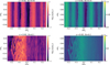 |
Fig. 2 Case of ϵ = 0.02, snapshots of the dust density (left) and Stokes number (right) for model E0v02S0v01c with St = 0.01 (left) and for model E0v02S0v1c with St = 0.1 (right). Both models include the effect of coagulation and result in the growth of the CI. |
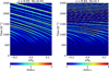 |
Fig. 3 Case of ϵ = 0.02, showing the time evolution of the vertically averaged dust density for model E0v02S0v01c with St = 0.01 (left), and model E0v02S0v1c with St = 0.1 (right). |
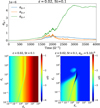 |
Fig. 4 Case of ϵ = 0.2 and St = 0.01 (model E0v02S0v01c), showing the time evolution of the dimensionless diffusion coefficients, αg,i, in each direction (top). The lower panel shows the expected linear growth rates for the same model in the inviscid case (left) and for αg,i = 5 × 10⁻⁶ (right). These have been obtained from linear theory (see Appendix A) using D = ν = αg,icsHg. Here, |
![Mathematical equation: $\[\tilde{K}_{x, z}=k_{x, z} \eta R_{0}\]$](/articles/aa/full_html/2026/02/aa58040-25/aa58040-25-eq32.png)
4.1.2 ϵ =0.2: Interplay between CI/SI and turbulence
In the case with ϵ = 0.2, we find that the difference in amplitude between the αg,i coefficients is smaller. For simulations including coagulation, their time evolution is represented in Fig. 6. The underlying turbulence is more isotropic in that case, with αg,y ~ αg,z for both St = 0.01 (Model E0v2S0v01c) and St = 0.1 (Model E0v2S0v1c). This is also illustrated in Fig. 7 where we plot the kinetic energy spectrum at saturation for St = 0.1. The power spectrum is broadly consistent with a negative five third power law (dashed line), which suggests Kolmogorov-like turbulence. Isotropic turbulence is expected for classical SI-driven turbulence, although we found an early evolution driven by the CI. In Fig. 1, the top-center and central panels show the evolution for St = 0.01 and St = 0.1, respectively. For models with coagulation, the initial rise in ϵmax (for t ≲ 100Ω−1 typically) is caused by the CI, involving density growth of vertically extended filaments through dust capture and merging of these filaments into denser ones. Compared to the previous case with ϵ = 0.02, however, it appears that the value for ϵmax is high enough to trigger the SI within the filaments, which leads to the subsequent increase in ϵmax that is observed. This would be consistent with the isotropic diffusion mentioned above. Figure 8 shows the dust density at the onset of the secondary increase in ϵmax. It is clear that nonlinear overdensities can grow in very localized regions within the filaments. This corresponds to unstable modes with vertical wavenumbers kz ≠ 0, which favors an SI-like instability. To confirm that the SI is definitely at work inside the filaments, we conducted a test calculation by restarting the run for St = 0.1 at t = 200Ω−1, but with the dust back-reaction onto the gas switched off. The results of this model indicate that the overdensities are quickly damped, which confirms the important role of the dust feedback for the formation of clumps in the filaments.
Interestingly, with respect to simulations without coagulation, we can notice that the overdensities that are produced by the SI in presence of coagulation are stronger. For St = 0.1 (middle-middle panel) and St = 0.01 (top-middle panel), models with coagulation yield ϵmax ≈ 6 and ϵmax ≈ 0.3–0.35, respectively, whereas the growth of the instability without coagulation is marginal. We argue that for this range of parameters, the SI may be assisted by dust coagulation. To support this argument, we present in Fig. 9 the growth rates of the SI (upper panel) and those obtained from our linear analysis with coagulation included (bottom panel), for St = 0.01. For the run with St = 0.1 (Model E0v2S0v1c), St = 0.01 corresponds roughly to the value for which overdensities start to grow inside the filaments (see middle-middle panel in Fig. 1). On this plot, the red-coloured rectangular region for ![Mathematical equation: $\[\tilde{K}_{x} \gtrsim 100\]$](/articles/aa/full_html/2026/02/aa58040-25/aa58040-25-eq35.png) , with
, with ![Mathematical equation: $\[\tilde{K}_{x}=k_{x} \eta R_{0}\]$](/articles/aa/full_html/2026/02/aa58040-25/aa58040-25-eq36.png) as the dimensionless wavenumber, corresponds to unstable CI modes as these modes have no vertical structure. The region enclosed between
as the dimensionless wavenumber, corresponds to unstable CI modes as these modes have no vertical structure. The region enclosed between ![Mathematical equation: $\[10 \lesssim \tilde{K}_{x} \lesssim 100\]$](/articles/aa/full_html/2026/02/aa58040-25/aa58040-25-eq37.png) and
and ![Mathematical equation: $\[10 \lesssim \tilde{K}_{z} \lesssim 100\]$](/articles/aa/full_html/2026/02/aa58040-25/aa58040-25-eq38.png) could, rather, be identified as unstable SI modes. Based on a comparison with the upper panel, we see that these modes have larger growth rates when coagulation is taken into account, which suggests that coagulation can amplify unstable SI modes. From Fig. 8, we estimate the typical radial extent of a vertically extended filament to be 0.02Hg, which corresponds to
could, rather, be identified as unstable SI modes. Based on a comparison with the upper panel, we see that these modes have larger growth rates when coagulation is taken into account, which suggests that coagulation can amplify unstable SI modes. From Fig. 8, we estimate the typical radial extent of a vertically extended filament to be 0.02Hg, which corresponds to ![Mathematical equation: $\[\tilde{K}_{x} \sim 15\]$](/articles/aa/full_html/2026/02/aa58040-25/aa58040-25-eq39.png) . This is well within this region of coagulation-assisted SI, confirming that this mechanism can indeed be at work here.
. This is well within this region of coagulation-assisted SI, confirming that this mechanism can indeed be at work here.
For St = 0.1 (Model E0v2S0v1c), inspecting the two panels of Fig. 8 reveals that the vertical filaments broaden with time, which is simply a consequence of turbulent diffusion generated by the coagulation-assisted SI. As the filaments spead out, they can subsequently start to intersect each other, which leads to an isotropic turbulent configuration as suggested by the middle panel of Fig. 10. We note that a similar evolution is found for St = 0.01, for which we show in the upper panel of Fig. 10 a snapshot of the dust density when the instability has saturated.
Going back to the middle panel Fig. 10, it is interesting to note that the fully turbulent state consists of large voids and narrow particle streams, which is similar to the patterns developed by the SI for strongly coupled particles (Johansen & Youdin 2007). For standard SI, however, this regime is typically found for ϵ ≳ 1 whereas for ϵ = 0.2, the dust density is left almost unchanged (see bottom panel of Fig. 10). This implies that coagulation makes this mode of nonlinear saturation of the SI occur at much lower dust-to-gas ratios. This is not surprising as coagulation tends to increase radial drift speed by increasing the Stokes number, so that growing particles can fall more rapidly through the voids created by Poisson fluctuations (Johansen & Youdin 2007). We note, however, that the dust density enhancement is limited to ~30–40 with coagulation included; whereas for standard SI, this mode of nonlinear saturation generally corresponds to strong clumping with dust density enhancements ≳100.
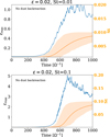 |
Fig. 5 Case of ϵ = 0.2, showing the time evolution of the maximum dust-to-gas ratio, ϵmax, and Stokes number for St = 0.01 (top) and St = 0.1 (bottom), where the effect of the dust backreaction onto the gas is discarded. |
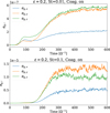 |
Fig. 6 Case of ϵ = 0.2, showing the time evolution of the dimensionless diffusion coefficients, αg,i, in each direction for models E0v2S0v01c with St = 0.01 (top) and E0v2S0v1c with St = 0.1 (bottom). |
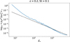 |
Fig. 7 Spectrum of the vertically averaged gas kinetic energy density for ϵ = 0.2 and St = 0.1 (run E0v2S0v1c). Here, |
![Mathematical equation: $\[\tilde{K}_{x}=k_{x} \eta R_{0}\]$](/articles/aa/full_html/2026/02/aa58040-25/aa58040-25-eq33.png)
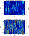 |
Fig. 8 For ϵ = 0.2 and St = 0.1 (run E0v2S0v1c, with coagulation), dust density snapshots at t = 120 Ω−1 (left) and t = 150 Ω−1 (right). |
 |
Fig. 9 Linear growth rates obtained from the linear analysis presented in Appendix A for ϵ = 0.2 and St = 0.01 for the case without coagulation (top) and with coagulation(bottom). Here, |
![Mathematical equation: $\[\tilde{K}_{x, z}=k_{x, z} \eta R_{0}\]$](/articles/aa/full_html/2026/02/aa58040-25/aa58040-25-eq34.png)
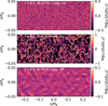 |
Fig. 10 Dust density map during the saturation phase for model E0v2S0v01c (ϵ = 0.2, St = 0.01, with coagulation), model E0v2S0v1c (ϵ = 0.2, St = 0.1, with coagulation), model E0v2S0v1 (ϵ = 0.2, St = 0.1, without coagulation), shown from top to bottom. |
4.2 Marginally coupled particles
For ϵ = 0.02, the evolution outcome of the model with final Stokes number St = 1 and including coagulation (run E0v02s1c, bottom left panel in Fig. 1) is found to be very similar to that of St = 0.1 particles (run E0v02s0v1c), involving the formation of a vertically extended filament inside which CI-induced turbulence operates.
For ϵ = 0.2, an interesting issue that emerges from the previous discussion (in Sect. 4.1.2) is whether the conditions needed to reach strong clumping are less stringent with coagulation. To investigate this further, we allowed, in the case where coagulation is included, the Stokes number to increase up to St = 1. For standard SI, a model with ϵ = 0.2 is expected to lie in the strong clumping regime for St ~ 1 and our main aim here is to examine if this threshold is diminished when coagulation is taken into account. In Fig. 1, models with ϵ = 0.2 and St = 1 correspond to the bottom middle panel where we compare the runs with and without coagulation. From this plot, it is immediately evident that: (i) the final outcome of the simulations does not depend on whether coagulation is included or not and (ii) including coagulation does not reduce the threshold in terms of Stokes number for the onset of strong clumping. Looking at the time evolution of ϵmax for the model with coagulation, we see that the initial behaviour is consistent with the results presented in the previous section, involving increase in ϵmax as coagulation-assisted SI grows and develops isotropic turbulence. At a later time, t ~ 200 Ω−1, however, ϵmax is observed to decrease before increasing again as St → 1. From the time evolution of St, we estimate the (mean) Stokes number associated with the observed drop of ϵmax occuring at t ~ 200 Ω−1 to be St ≈ 0.3. Interestingly, we find by running simulations of standard SI with different Stokes numbers that this value coincides approximately with the one above which significant growth of the SI occurs. To explore the origin of this decrease in ϵmax in more details, we have conducted a number of test calculations, by restarting the simulation with coagulation (run E0v2S1c) at t ~ 200 Ω−1, but with dust coagulation (feedback) switched on (off). The findings of this study can be summarised as follows:
a restarted run with dust backreaction onto the gas switched off leads to a continuous increase in ϵmax due to CI, which is the opposite behaviour to that found in model E0v2S1c. This demonstrates that dust feedback plays an important role in the decrease in ϵmax seen in run E0v2S1c;
a restarted run with dust coagulation switched off results in the development of the SI into stripes aligned in the vertical direction but tilted in the radial direction, similarly to the patterns formed by the SI in the case of large particles (Johansen & Youdin 2007). When applied to run E0v2S1c, this shows that from t ~ 200 Ω−1 onward, the SI can indeed be triggered, consistenly with the results of our simulations of standard SI with various Stokes numbers. During the saturated state, we find ϵmax ~ 0.5–1 for this test calculation, which is also in agreement with our standard SI calculation with St = 0.3;
a restarted run with coagulation and dust backreaction switched off results in a maintained quasi-stationary turbulent state, with ϵmax remaining close to its initial value.
Taken together, these results suggest that provided its growth rate is high enough, the SI can counteract the effect of the CI such that the final turbulent state is similar to that found in pure SI calculations. This is illustrated in Fig. 11, which shows the evolution of the dust density for the model with coagulation included (run E0v2S1c). The large stripes tilted toward the vertical direction that are expected to develop during nonlinear saturation of the SI for St = 1 particles can easily be recognized. For the particular model with ϵ = 0.2 and St = 1, examining Table 1 confirms that the values αSS and αg,i do not depend on whether or not coagulation is included.
To clearly demonstrate the finding that the SI can overcome the effects of the CI, we show in Fig. 12 linear growth rates of the instability for ϵ = 0.2 and two different values of St. Here, both the CI and SI operate, with the unstable CI (resp. SI) modes corresponding to the unstable modes that have little (resp. strong) dependence on ![Mathematical equation: $\[\tilde{K}_{z}\]$](/articles/aa/full_html/2026/02/aa58040-25/aa58040-25-eq41.png) . We see that as coagulation proceeds and Stokes number transitions from St = 0.3 to St = 1, the maximum growth rate of the SI increases whereas unstable CI modes with radial wavenumbers in the range
. We see that as coagulation proceeds and Stokes number transitions from St = 0.3 to St = 1, the maximum growth rate of the SI increases whereas unstable CI modes with radial wavenumbers in the range ![Mathematical equation: $\[\tilde{K}_{x} \in[5-100]\]$](/articles/aa/full_html/2026/02/aa58040-25/aa58040-25-eq42.png) are damped. This possibly arises because both CI and SI are driven by the radial drift of dust, which acts as a finite energy reservoir for the two instabilities such that any of these two instabilities can only grow at the expense of the other.
are damped. This possibly arises because both CI and SI are driven by the radial drift of dust, which acts as a finite energy reservoir for the two instabilities such that any of these two instabilities can only grow at the expense of the other.
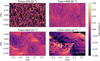 |
Fig. 11 Case of ϵ = 0.2 and St = 1 (model E0v2S1c, with coagulation), with dust density snapshots taken at different times. |
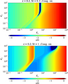 |
Fig. 12 Case ϵ = 0.2, including the effects of coagulation, along with the linear growth rates obtained from the linear analysis presented in Appendix A for St = 0.3 (top) and St = 1 (bottom). Here, |
![Mathematical equation: $\[\tilde{K}_{x, z}=k_{x, z} \eta R_{0}\]$](/articles/aa/full_html/2026/02/aa58040-25/aa58040-25-eq40.png)
5 Discussion
5.1 Impact of coagulation on the streaming instability
Although a model with ϵ = 0.2 and St = 1 leads to strong clumping, consistently with the results of Johansen & Youdin (2007), a necessary condition for particle clumping through the SI is generally approximated as ϵ ≳ 1 in the disk midplane, due to the strong increase in the SI linear growth rates at ϵ ≈ 1 for St ≲ 1. The right panels of Fig. 1 show the effect of coagulation on the SI for ϵ = 3. The SI linear growth rate for St = 0.01 is σ ~ Ω−1 but this case only produced modest overdensities, whereas strong clumping occurred for St ≳ 0.1, as expected. Clearly, the effect of coagulation appears to be negligible for ϵ = 3, regardless the (final) value for St. Combined with our results for ϵ = 0.2 and St = 1, this suggests that for the optimally dust sizes and dust-to-gas ratios that maximize the SI growth rate, coagulation has an almost null effect. In that case, this means not only that i) coagulation has no impact on the SI linear growth rate, but also that ii) the dust concentration at saturation is not affected by coagulation. Physically, this arises simply when the coagulation timescale is longer that the SI growth timescale or, equivalently, when the particule coagulation growth rate is smaller than the SI growth rate. From Eq. (8), the inverse of the coagulation timescale is approximately given by
![Mathematical equation: $\[t_{\mathrm{coag}}^{-1}=\frac{1}{2} \sqrt{\frac{\pi \alpha C}{8 \mathrm{St}}} \epsilon.\]$](/articles/aa/full_html/2026/02/aa58040-25/aa58040-25-eq43.png) (26)
(26)
For St = 0.01 this leads to ![Mathematical equation: $\[t_{\text {coag }}^{-1} \sim 0.01 \Omega^{-1}\]$](/articles/aa/full_html/2026/02/aa58040-25/aa58040-25-eq44.png) , which is indeed smaller that the aforementioned SI growth rate. Starting from an initial Stokes number St = 10−3, coagulation can of course promote SI by increasing the average dust size by one to two orders of magnitude, consistently with the results of Ho et al. (2024). However, we find that once the SI is triggered, its dynamics dominate over coagulation effects.
, which is indeed smaller that the aforementioned SI growth rate. Starting from an initial Stokes number St = 10−3, coagulation can of course promote SI by increasing the average dust size by one to two orders of magnitude, consistently with the results of Ho et al. (2024). However, we find that once the SI is triggered, its dynamics dominate over coagulation effects.
5.2 Effect of coagulation on turbulence and dust diffusion
Nevertheless, we have also shown that under certain conditions, coagulation and SI can act in concert. This is particularly true in dust-poor disks where the SI can grow in the vertically extended filaments formed by the CI, leading to a regime of coagulation-assisted SI that ultimately results in a level of turbulence much higher compared to standard SI (see Sect. 4.1.2). For each model, the αSS dimensionless parameter that quantities the radial flux of gas orbital momentum is listed in the first column of Table 1. Most runs have αSS < 0, in agreement with previous estimations of the flux of angular momentum in SI-driven turbulent disks (Johansen & Youdin 2007; Hsu & Lin 2022). The fact that αSS is more negative when coagulation is taken into account suggests that the radial transport of angular momentum induced by the CI is also inward. This is not surprising since, similarly to the SI (Johansen & Youdin 2007), CI is also powered by a global pressure gradient.
An interesting issue that needs to be investigated is how the collision velocity resulting from the turbulence compares with the fragmentation velocity, vf. It can indeed not be excluded that the turbulence driven by the coagulation and streaming instabilities in turn hinders further coagulation by producing collision velocities that exceed the fragmentation threshold. To address this question, we can estimate the maximum Stokes number, Stf, achievable through coagulation. From Eq. (9), it is straightforward to show that Stf is given by
![Mathematical equation: $\[\mathrm{St}_f=\frac{v_f^2}{C \alpha_{\mathrm{SS}} c_s^2}.\]$](/articles/aa/full_html/2026/02/aa58040-25/aa58040-25-eq45.png) (27)
(27)
The fragmentation velocity has been studied both numerically and experimentally (Blum & Wurm 2008; Zsom et al. 2010; Wada et al. 2013; Gundlach & Blum 2015; Ueda et al. 2019), and it has been estimated to be between 1 and 10 m s−1 for silicate particles and between 10 and 80 m s−1 for icy aggregates. Regardless the nature of dust aggregates, all but one simulation resulted in turbulent collision velocities smaller than vf for typical disk parameters. Assuming that R0 corresponds to 1 AU, Model E0v2S0v1c which enters the regime of coagulation-assisted SI is the only exception, as we find Stf ≈ 0.07 for vf = 1 m s−1. By preventing the formation of large dust grains, this implies that coagulation-driven turbulence may in that case inhibit the strong clumping phase of the SI.
A related effect of coagulation is the vertical diffusion of particles driven by the CI and/or SI. At a steady state (i.e., once turbulent diffusion counterbalances gravitational settling), it is expected that the particle profile is characterized by a dust scale height, Hd, given by (Dubrulle et al. 1995; Youdin & Lithwick 2007):
![Mathematical equation: $\[\frac{H_d}{H_g}=\sqrt{\frac{\alpha_{g, z}}{\alpha_{g, z}+\mathrm{St}}}.\]$](/articles/aa/full_html/2026/02/aa58040-25/aa58040-25-eq46.png) (28)
(28)
Using the values for αg,z reported in Table 1, we find that it is possible to differentiate between CI and SI in dust-poor disks with ϵ ≲ 0.2 and for tightly coupled particles with St ≲ 0.1, as the SI is ineffective at producing a significant level of turbulence under these conditions. In contrast, the CI on its own can generate a vertical bulk diffusion coefficient αgz ~ 5 × 10⁻⁷ for ϵ = 0.02, which results in Hd ~ 0.006Hg. In the coagulation-assisted SI regime (run E0v2S0v1c), αg,z can even reach 𝒪(10−4) for St = 0.1, corresponding to Hd ~ 0.01Hg.
5.3 Caveats
The results that we presented in this work may suffer from a number of assumptions and limitations, the main one being that we adopted a moment equation to describe dust coagulation, based on the vertically integrated Smoluchowski equation (Sato et al. 2016; Tominaga et al. 2021). Rather than focusing on the evolution of the full dust size distribution, this approach consists in following the evolution of the so-called peak mass, which represents the weighted average mass. Sato et al. (2016) have shown that provided the effect of finite size dispersion is taken into account when evaluating the collision velocities, good agreement is obtained between single-size and full size calculations of drifting and growing dust grains in protoplanetary disks. We caution, however, that the original model of Sato et al. (2016) does not take into account the effect of fragmentation and it is not clear whether or not the single-size approximation would still hold when fragmentation is considered, since this process would tend to broaden the initial dust size distribution. Relaxing the single-size approximation and considering a full, possibly wide, dust size distribution produced by fragmentation may have important consequences on our results. In the context of the SI, recent studies have shown that taking into account the effect of a dust size distribution can significantly modify the growth rate of (monodisperse) SI (Krapp et al. 2019; Paardekooper et al. 2020; Zhu & Yang 2021; McNally et al. 2021). Therefore, our model does not have the capacity to explore the effect of coagulation on this “polydisperse” SI and this should be examined in a future study.
We also considered inviscid disks, while various hydrodynamical instabilities can be triggered in the planet-forming regions of protoplanetary disks. This gives rise to turbulence, with a corresponding turbulent viscosity, typically leading to αSS ~ 10−4. These levels of external turbulence may significantly impact the nonlinear evolution of both the SI (Chen & Lin 2020), and CI (Tominaga et al. 2021). Although models that include dissipation effects should be explored in more detail, we present in Appendix B the results of a few viscous simulations that also take dust diffusion into account. This suggests that the results presented in this paper could be affected by the external turbulence for αSS ≳ 10−6.
Another limitation lies in the size of our vertical domain that is (based on the discussion in Sect. 5.2) systematically higher than the dust layer thickness. The consequence of this is that the effects of stratification might be important and these should be examined in more details in a future study. Another reason for considering vertically stratified disks is that the CI is characterised by vertically extended filaments and it is not clear whether or not these would persist in stratified models.
We note that these two aspects, namely, considering a full dust size distribution and vertical stratification, were recently studied by Ho et al. (2024). Although the potential important effect of the CI was not investigated in this work, they found that the dust size distribution can be significantly altered by coagulation within the dense dust clumps that are formed as the dust settles toward the midplane and the SI is triggered.
6 Summary
In this paper, we present the results of unstratified, axisymmetric, shearing-box simulations of SI including the effect of dust coagulation. We solved a simplified version of the coagulation equation by a moment method, which consists of following the size evolution of solids that dominate the total dust surface density. Our primary aim was to examine to what extent dust growth impacts the linear growth of the SI and to get insight into its impact on the nonlinear saturation phase of the SI. We are particularly interested in the role played by the CI (Tominaga et al. 2021), which results from the dust-density dependence of coagulation efficiency and the grain size dependence of radial drift speed. Our motivation stems from the fact that the CI can be triggered for dust-to-gas ratios as small as ϵ ~ 10−3 and make the Stokes number of solids rapidly reach unity, leading thereby to optimal conditions for efficient growth of the SI. We studied how the CI and the SI can interact with each other, as well as how the interplay between these two instabilities depends on the initial dust-to-gas ratio and on the maximum Stokes number St allowed before fragmentation sets in. Our key findings are summarized as follows:
In dust-poor disks with ϵ ~ 10−2 and for tightly coupled particles with St ≲ 10−1, we find that evolution is mainly driven by the CI. Since the latter instability is by essence an axisymmetric instability, early evolution involves the formation of vertically extended filaments that tend to merge themselves more rapidly for larger Stokes numbers. Within the filaments, the nonlinear saturation of the CI gives rise to anisotropic turbulence with an enhanced dust diffusion coefficient in the vertical direction;
In dust-rich disks with ϵ > 1, evolution is mainly driven by the SI simply because in that case, the growth timescale of the SI is smaller than the coagulation timescale. In this regime, coagulation is observed to have only little effect, not only on the initial linear growth rate of the instability, but also on the final dust concentration values reached once the SI has saturated;
For intermediate dust-to-gas ratios of ϵ ~ 0.1 and Stokes numbers St ≲ 0.1, we observe the onset of the SI within the filaments formed originally by the CI. An examination of linear growth rate maps indicates that for this range of parameters, the linear growth rate of the SI is significantly increased by coagulation effects, which we refer to as a regime of coagulation-assisted SI. In this regime, nonlinear evolution leads to isotropic turbulence with dust diffusion coefficients having similar value in each direction. The generated turbulence causes the vertically extended filaments to spread out until they start to intersect each other, ultimately leading to a turbulent state characterised by large voids and narrow particle streams. The patterns that develop look similar to those formed by the SI in the strong clumping regime, albeit with a smaller dust concentration, on the order of 𝒪(30–40), compared to that typical of the strong clumping regime;
However, as the Stokes number increases and approaches unity, SI can overcome the effect of the CI. Thus, the final turbulent state ends up being very similar to the results of pure SI calculations without the effect of coagulation included.
Taken together, these findings suggest that the formation of dense clumps through the SI may be rendered easier by coagulation, simply because the process of dust growth enables the SI to reside in a regime where it can operate efficiently. The CI on its own only has a slight impact on the onset of the SI, but it can nonetheless be a non negligible source of turbulence in protoplanetary disks, especially when it acts in concert with the SI.
Acknowledgements
Computer time for this study was provided by the computing facilities MCIA (Mésocentre de Calcul Intensif Aquitain) of the Universite de Bordeaux and by HPC resources of Cines under the allocation A0170406957 made by GENCI (Grand Equipement National de Calcul Intensif). MKL is supported by the National Science and Technology Council (grants 113-2112-M-001-036-, 114-2112-M-001-018-, 113-2124-M-002-003-, 114-2124-M-002-003-) and an Academia Sinica Career Development Award (AS-CDA-110-M06). This work was partly supported by the “Action Thématique de Physique Stellaire” (ATPS) of CNRS/INSU PN Astro co-funded by CEA and CNES, and by ORCHID program (project number: 49523 PG, co-PI. Dutrey-Tang), funded by the French Ministry for Europe and Foreign Affairs, the French Ministry for Higher Education and Research and the National Science and Technology Council (NSTC).
References
- Abod, C. P., Simon, J. B., Li, R., et al. 2019, ApJ, 883, 192 [Google Scholar]
- Benítez-Llambay, P., & Masset, F. S. 2016, ApJS, 223, 11 [Google Scholar]
- Benítez-Llambay, P., Krapp, L., & Pessah, M. E. 2019, ApJS, 241, 25 [Google Scholar]
- Blum, J., & Wurm, G. 2008, ARA&A, 46, 21 [CrossRef] [Google Scholar]
- Carrera, D., Johansen, A., & Davies, M. B. 2015, A&A, 579, A43 [NASA ADS] [CrossRef] [EDP Sciences] [Google Scholar]
- Carrera, D., Lim, J., Eriksson, L. E. J., Lyra, W., & Simon, J. B. 2025, A&A, 696, L23 [NASA ADS] [CrossRef] [EDP Sciences] [Google Scholar]
- Chen, K., & Lin, M.-K. 2020, ApJ, 891, 132 [Google Scholar]
- Drążkowska, J., & Dullemond, C. P. 2014, A&A, 572, A78 [NASA ADS] [CrossRef] [EDP Sciences] [Google Scholar]
- Dubrulle, B., Morfill, G., & Sterzik, M. 1995, Icarus, 114, 237 [Google Scholar]
- Dullemond, C. P., & Dominik, C. 2005, A&A, 434, 971 [CrossRef] [EDP Sciences] [Google Scholar]
- Fromang, S., & Papaloizou, J. 2006, A&A, 452, 751 [NASA ADS] [CrossRef] [EDP Sciences] [Google Scholar]
- Gundlach, B., & Blum, J. 2015, ApJ, 798, 34 [Google Scholar]
- Ho, K. W., Li, H., & Li, S. 2024, ApJ, 975, L34 [Google Scholar]
- Hsu, C.-Y., & Lin, M.-K. 2022, ApJ, 937, 55 [Google Scholar]
- Johansen, A., & Youdin, A. 2007, ApJ, 662, 627 [Google Scholar]
- Johansen, A., Youdin, A., & Mac Low, M.-M. 2009, ApJ, 704, L75 [NASA ADS] [CrossRef] [Google Scholar]
- Krapp, L., Benítez-Llambay, P., Gressel, O., & Pessah, M. E. 2019, ApJ, 878, L30 [Google Scholar]
- Li, R., & Youdin, A. N. 2021, ApJ, 919, 107 [NASA ADS] [CrossRef] [Google Scholar]
- Lin, M.-K., & Youdin, A. N. 2017, ApJ, 849, 129 [NASA ADS] [CrossRef] [Google Scholar]
- McNally, C. P., Lovascio, F., & Paardekooper, S.-J. 2021, MNRAS, 502, 1469 [NASA ADS] [CrossRef] [Google Scholar]
- Nakagawa, Y., Sekiya, M., & Hayashi, C. 1986, Icarus, 67, 375 [Google Scholar]
- Ormel, C. W., & Cuzzi, J. N. 2007, A&A, 466, 413 [NASA ADS] [CrossRef] [EDP Sciences] [Google Scholar]
- Paardekooper, S.-J., McNally, C. P., & Lovascio, F. 2020, MNRAS, 499, 4223 [CrossRef] [Google Scholar]
- Sato, T., Okuzumi, S., & Ida, S. 2016, A&A, 589, A15 [NASA ADS] [CrossRef] [EDP Sciences] [Google Scholar]
- Shakura, N. I., & Sunyaev, R. A. 1973, A&A, 24, 337 [NASA ADS] [Google Scholar]
- Simon, J. B., Armitage, P. J., Li, R., & Youdin, A. N. 2016, ApJ, 822, 55 [Google Scholar]
- Tominaga, R. T., & Tanaka, H. 2023, ApJ, 958, 168 [Google Scholar]
- Tominaga, R. T., & Tanaka, H. 2025, ApJ, 983, 15 [Google Scholar]
- Tominaga, R. T., Inutsuka, S.-i., & Kobayashi, H. 2021, ApJ, 923, 34 [NASA ADS] [CrossRef] [Google Scholar]
- Tominaga, R. T., Kobayashi, H., & Inutsuka, S.-i. 2022a, ApJ, 937, 21 [Google Scholar]
- Tominaga, R. T., Tanaka, H., Kobayashi, H., & Inutsuka, S.-i. 2022b, ApJ, 940, 152 [NASA ADS] [CrossRef] [Google Scholar]
- Ueda, T., Flock, M., & Okuzumi, S. 2019, ApJ, 871, 10 [Google Scholar]
- Wada, K., Tanaka, H., Okuzumi, S., et al. 2013, A&A, 559, A62 [NASA ADS] [CrossRef] [EDP Sciences] [Google Scholar]
- Yang, C.-C., Johansen, A., & Carrera, D. 2017, A&A, 606, A80 [NASA ADS] [CrossRef] [EDP Sciences] [Google Scholar]
- Yang, C.-C., Mac Low, M.-M., & Johansen, A. 2018, ApJ, 868, 27 [NASA ADS] [CrossRef] [Google Scholar]
- Youdin, A. N., & Goodman, J. 2005, ApJ, 620, 459 [Google Scholar]
- Youdin, A., & Johansen, A. 2007, ApJ, 662, 613 [Google Scholar]
- Youdin, A. N., & Lithwick, Y. 2007, Icarus, 192, 588 [NASA ADS] [CrossRef] [Google Scholar]
- Zhu, Z., & Yang, C.-C. 2021, MNRAS, 501, 467 [Google Scholar]
- Zsom, A., Ormel, C. W., Güttler, C., Blum, J., & Dullemond, C. P. 2010, A&A, 513, A57 [NASA ADS] [CrossRef] [EDP Sciences] [Google Scholar]
Appendix A Linearized equations
To linearize Eqs. 1–4, we write X as a quantity of the system as the sum between the equilibrium state X0 (Eqs. 11–14), and a perturbation δX << X0 in Fourier modes with kx and kz the spatial modes and σ the growth rate of the instability.
![Mathematical equation: $\[X(x, z, t)=X_0(x, z)+\delta X \times e^{i\left(k_x x+k_z z\right)+\sigma t}.\]$](/articles/aa/full_html/2026/02/aa58040-25/aa58040-25-eq47.png) (A.1)
(A.1)
By injecting this into the mass continuity equations, Eqs. 1 and 3, we obtain
![Mathematical equation: $\[\sigma \delta \rho_g=-\rho_{g, 0}\left(i k_x \delta u_x+i k_z \delta u_z\right)-i k_x u_{x, 0} \delta \rho_g,\]$](/articles/aa/full_html/2026/02/aa58040-25/aa58040-25-eq48.png) (A.2a)
(A.2a)
![Mathematical equation: $\[\begin{aligned}\sigma \delta \rho_d= & -\rho_{d, 0}\left(i k_x \delta v_x+i k_z \delta v_z\right)-i k_x v_{x, 0} \delta \rho_d \\& -\rho_{d, 0} D\left(k_x^2+k_z^2\right)\left(\delta \rho_d / \rho_{d, 0}-\delta \rho_g / \rho_{g, 0}\right).\end{aligned}\]$](/articles/aa/full_html/2026/02/aa58040-25/aa58040-25-eq49.png) (A.2b)
(A.2b)
Similarly, with the equations of conservation of momentum for the gas Eq. 2
![Mathematical equation: $\[\begin{aligned}\sigma \delta u_x= & -u_{x, 0} i k_x \delta u_x+2 \Omega \delta u_y-c_s^2 i k_x \frac{\delta \rho_g}{\rho_{g, 0}}+\delta F_x^{v i s c} \\& -C_{D F} m_p^{-1 / 3}\left\{\left[\delta \rho_d-\frac{1}{3 m_p} \rho_d \delta m_p\right]\left(u_{x, 0}-v_{x, 0}\right)\right. \\&\qquad\qquad\qquad \left.+\rho_d\left(\delta u_x-\delta v_x\right)\right\},\end{aligned}\]$](/articles/aa/full_html/2026/02/aa58040-25/aa58040-25-eq50.png) (A.3a)
(A.3a)
![Mathematical equation: $\[\begin{aligned}\sigma \delta u_y= & -u_{x, 0} i k_x \delta u_y-\frac{1}{2} \Omega \delta u_x+\delta F_y^{v i s c} \\& -C_{D F} m_p^{-1 / 3}\left\{\left[\delta \rho_d-\frac{1}{3 m_p} \rho_d \delta m_p\right]\left(u_{y, 0}-v_{y, 0}\right)\right. \\&\qquad\qquad\qquad \left.+\rho_d\left(\delta u_y-\delta v_y\right)\right\},\end{aligned}\]$](/articles/aa/full_html/2026/02/aa58040-25/aa58040-25-eq51.png) (A.3b)
(A.3b)
![Mathematical equation: $\[\begin{aligned}\sigma \delta u_z= & -u_{x, 0} i k_x \delta u_z-c_s^2 i k_z \frac{\delta \rho_g}{\rho_{g, 0}}+\delta F_z^{v i s c} \\& -C_{D F} m_p^{-1 / 3} \rho_d\left(\delta u_z-\delta v_z\right),\end{aligned}\]$](/articles/aa/full_html/2026/02/aa58040-25/aa58040-25-eq52.png) (A.3c)
(A.3c)
with ![Mathematical equation: $\[C_{D F}=\Omega \sqrt{\frac{8}{\pi}} \frac{H_{g}}{\rho_{i}}\left(\frac{4 \pi \rho_{i}}{3}\right)^{1 / 3}\]$](/articles/aa/full_html/2026/02/aa58040-25/aa58040-25-eq53.png) a coefficient related to drag force and
a coefficient related to drag force and ![Mathematical equation: $\[\delta F_{(x, y, z)}^{v i s c}\]$](/articles/aa/full_html/2026/02/aa58040-25/aa58040-25-eq54.png) the linearized viscous forces from Chen & Lin (2020):
the linearized viscous forces from Chen & Lin (2020):
![Mathematical equation: $\[\delta F_x^{v i s c}=-\nu\left(k_z^2+\frac{4}{3} k_x^2\right) \delta v_x-\frac{1}{3} v k_x k_z \delta v_z,\]$](/articles/aa/full_html/2026/02/aa58040-25/aa58040-25-eq55.png) (A.4a)
(A.4a)
![Mathematical equation: $\[\delta F_y^{v i s c}=-\nu\left(k_z^2+k_x^2\right) \delta v_y,\]$](/articles/aa/full_html/2026/02/aa58040-25/aa58040-25-eq56.png) (A.4b)
(A.4b)
![Mathematical equation: $\[\delta F_z^{v i s c}=-\nu\left(\frac{4}{3} k_z^2+k_x^2\right) \delta v_z-\frac{1}{3} \nu k_x k_z \delta v_x,\]$](/articles/aa/full_html/2026/02/aa58040-25/aa58040-25-eq57.png) (A.4c)
(A.4c)
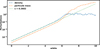 |
Fig. A.1 Perturbation |
![Mathematical equation: $\[\frac{max (\left|\rho_{d}-\rho_{d, 0}\right|)}{\rho_{d, 0}}\]$](/articles/aa/full_html/2026/02/aa58040-25/aa58040-25-eq58.png)
![Mathematical equation: $\[\frac{max (\left|m_{p}-m_{p, 0}\right|)}{m_{p, 0}}\]$](/articles/aa/full_html/2026/02/aa58040-25/aa58040-25-eq59.png)
and for the equations of conservation of momentum for the dust Eq. 4,
![Mathematical equation: $\[\begin{aligned}\sigma \delta v_x= & -v_{x, 0} i k_x \delta v_x+2 \Omega \delta v_y \\& -C_{D F} m_p^{-1 / 3}\left\{\left[\delta \rho_g-\frac{1}{3 m_p} \rho_g \delta m_p\right]\left(v_{x, 0}-u_{x, 0}\right)\right. \\&\qquad\qquad\qquad \left.+\rho_g\left(\delta v_x-\delta u_x\right)\right\},\end{aligned}\]$](/articles/aa/full_html/2026/02/aa58040-25/aa58040-25-eq60.png) (A.5a)
(A.5a)
![Mathematical equation: $\[\begin{aligned}\sigma \delta v_y= & -v_{x, 0} i k_x \delta v_y-\frac{1}{2} \Omega \delta v_x \\& -C_{D F} m_p^{-1 / 3}\left\{\left[\delta \rho_g-\frac{1}{3 m_p} \rho_g \delta m_p\right]\left(v_{y, 0}-u_{y, 0}\right)\right. \\&\qquad\qquad\qquad \left.+\rho_g\left(\delta v_y-\delta u_y\right)\right\},\end{aligned}\]$](/articles/aa/full_html/2026/02/aa58040-25/aa58040-25-eq61.png) (A.5b)
(A.5b)
![Mathematical equation: $\[\sigma \delta v_z=-v_{x, 0} i k_x \delta v_z-C_{D F} m_p^{-1 / 3} \rho_g\left(\delta v_z-\delta u_z\right).\]$](/articles/aa/full_html/2026/02/aa58040-25/aa58040-25-eq62.png) (A.5c)
(A.5c)
And finally, the perturbed equation for the coagulation equation, expressed in Eq. 8,
![Mathematical equation: $\[\sigma \delta m_p=-v_{x, 0} i k_x \delta m_p+D_{coag} m_p^{5 / 6} \rho_g^{-1 / 2} \rho_d\left[\frac{5}{6} \frac{\delta m_p}{m_p}-\frac{1}{2} \frac{\delta \rho_g}{\rho_g}+\frac{\delta \rho_d}{\rho_d}\right],\]$](/articles/aa/full_html/2026/02/aa58040-25/aa58040-25-eq63.png) (A.6)
(A.6)
with ![Mathematical equation: $\[D_{coag}=\left(\frac{\pi}{2}\right)^{5 / 12} \times 3^{5 / 6} \rho_{i}^{-1 / 3} \sqrt{2.3 \alpha} H_{g}^{-1 / 2} c_{s}\]$](/articles/aa/full_html/2026/02/aa58040-25/aa58040-25-eq64.png) .
.
This system of nine equations is rewritten in its matrix form as sV = AV, using the dimensionless quantities ![Mathematical equation: $\[\hat{v}= \frac{v}{\eta R \Omega}, K=k \eta R\]$](/articles/aa/full_html/2026/02/aa58040-25/aa58040-25-eq65.png) and
and ![Mathematical equation: $\[s=\frac{\sigma}{\Omega}\]$](/articles/aa/full_html/2026/02/aa58040-25/aa58040-25-eq66.png) , with the perturbation vector
, with the perturbation vector ![Mathematical equation: $\[\mathbf{V}=\left[\frac{\delta \rho_{g}}{\rho_{g}}, \quad \frac{\delta \rho_{d}}{\rho_{d}}, \quad \delta \hat{u}_{x}, \quad \delta \hat{u}_{y}, \quad \delta \hat{u}_{z}, \quad \delta \hat{v}_{x}, \quad \delta \hat{v}_{y}, \quad \delta \hat{v}_{z}, \quad \frac{\delta m_{p}}{m_{p}}\right]^{\top}\]$](/articles/aa/full_html/2026/02/aa58040-25/aa58040-25-eq67.png) and the matrix of the linearized system A.
and the matrix of the linearized system A.
For a given spatial mode (Kx, Kz), the largest eigenvalue of A corresponds to the growth rate σ of the most unstable mode, while the associated eigenvector can be used to study the linear case of this mode numerically. This enables a verification of the coagulation implementation, as well as the analytical development growth rates derived from the matrix’s eigenvalues via a comparison of the two, as done in Fig. A.1 in the linA case of St = 0.1, ϵ = 3 and (Kx, Kz) = (30, 30) with coagulation. The analytical solution gives s = 0.3602, identical to the numerical growth rate derived from the particle density and particle mass until the perturbation is no longer negligible (δX ~ 0.1).
Appendix B Effect of gas viscosity and dust diffusion
In the inviscid limit that we considered in this work, the numerical dissipation may impact our results, such that these could be dependent on the employed resolution. This is because the growth rate of CI increases with radial wavenumber, such that the maximum wavenumber that is resolved by the grid is expected to be unstable. Here, we present the results of additional simulations with nonzero gas viscosity, parameterized as ν = αcSHg, and with the dust diffusion coefficient set to the same value, namely, D = ν. As in inviscid simulations presented above, the αcoag parameter introduced into Eq. 9 is set to αcoag = 10−4. The aim here is to examine: i) how the results are changed when dissipation processes are controlled and ii) how these would be modified in presence of external turbulence, namely when the turbulence originates from other sources of instabilities than the CI and/or SI individually. For different values of the standard α parameter, the time evolution of ϵmax and st for these runs is presented in Fig. B.1. Not surprisingly, the linear growth rate of the instabilities is reduced as α is increased. This is a consequence of the stabilization of the CI by dust diffusion (Tominaga et al. 2021). Unstable high wavenumbers modes are also suppressed, as illustrated by Fig. B.2, which shows the dust density at the end of the linear growth phase. From Fig. B.1, we estimate the value for the numerical viscosity to correspond to α ~ 10−9–10−7. This is in line with the expectation that unstable modes with wavenumbers such that ![Mathematical equation: $\[k H \sim 1 / \sqrt{\alpha}\]$](/articles/aa/full_html/2026/02/aa58040-25/aa58040-25-eq68.png) are damped by turbulence (Dubrulle et al. 1995). Using α = 10−7, this gives kH ≈ 3 × 10³, which is close to the value mentioned in Sect. 4.1.1. Going back to Fig. B.1, we can observe growth of the SI for each value of α we considered, except for α = 10−6. In that case, however, St ≲ 0.5 at the end of the simulation due to slower coagulation, leading to a reduced SI growth rate. As St → 1, the SI should nevertheless enter a strong clumping regime, as it is expected in that case the SI growth rate to be only impacted by diffusion for α = 10−6 (e.g., see the upper-left panel of Fig. 3. in Chen & Lin 2020).
are damped by turbulence (Dubrulle et al. 1995). Using α = 10−7, this gives kH ≈ 3 × 10³, which is close to the value mentioned in Sect. 4.1.1. Going back to Fig. B.1, we can observe growth of the SI for each value of α we considered, except for α = 10−6. In that case, however, St ≲ 0.5 at the end of the simulation due to slower coagulation, leading to a reduced SI growth rate. As St → 1, the SI should nevertheless enter a strong clumping regime, as it is expected in that case the SI growth rate to be only impacted by diffusion for α = 10−6 (e.g., see the upper-left panel of Fig. 3. in Chen & Lin 2020).
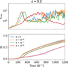 |
Fig. B.1 For ϵ = 0.2, St = 1 and with coagulation included, time evolution of the maximum dust-to-gas ratio ϵmax and Stokes number St in viscous simulations where the α viscous stress parameter is taken to be equal to the dimensionless dust diffusion coefficient. |
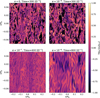 |
Fig. B.2 For ϵ = 0.2, St = 1, dust density snapshots for the reference inviscid run (top-left) and for viscous simulations with α = 10−9 (top-right), α = 10−7 (bottom-left), and α = 10−6 (bottom-right). |
All Tables
All Figures
|
Fig. 1 Time evolution of the maximum dust-to-gas ratio, ϵmax, and Stokes number for all simulations listed in Table 1. The left, middle, and right columns correspond to ϵ = 0.02, 0.2, 3, respectively, while the upper, middle, and lower panels correspond to St = 0.01, 0.1, 1 respectively. In each panel, we show the evolution of ϵmax for the case with (blue) and without (green) coagulation. For the evolution of St, the light colour traces the minimum and maximum values, whereas the dark colour traces the box averaged value. |
| In the text | |
|
Fig. 2 Case of ϵ = 0.02, snapshots of the dust density (left) and Stokes number (right) for model E0v02S0v01c with St = 0.01 (left) and for model E0v02S0v1c with St = 0.1 (right). Both models include the effect of coagulation and result in the growth of the CI. |
| In the text | |
|
Fig. 3 Case of ϵ = 0.02, showing the time evolution of the vertically averaged dust density for model E0v02S0v01c with St = 0.01 (left), and model E0v02S0v1c with St = 0.1 (right). |
| In the text | |
|
Fig. 4 Case of ϵ = 0.2 and St = 0.01 (model E0v02S0v01c), showing the time evolution of the dimensionless diffusion coefficients, αg,i, in each direction (top). The lower panel shows the expected linear growth rates for the same model in the inviscid case (left) and for αg,i = 5 × 10⁻⁶ (right). These have been obtained from linear theory (see Appendix A) using D = ν = αg,icsHg. Here, |
| In the text | |
|
Fig. 5 Case of ϵ = 0.2, showing the time evolution of the maximum dust-to-gas ratio, ϵmax, and Stokes number for St = 0.01 (top) and St = 0.1 (bottom), where the effect of the dust backreaction onto the gas is discarded. |
| In the text | |
|
Fig. 6 Case of ϵ = 0.2, showing the time evolution of the dimensionless diffusion coefficients, αg,i, in each direction for models E0v2S0v01c with St = 0.01 (top) and E0v2S0v1c with St = 0.1 (bottom). |
| In the text | |
|
Fig. 7 Spectrum of the vertically averaged gas kinetic energy density for ϵ = 0.2 and St = 0.1 (run E0v2S0v1c). Here, |
| In the text | |
|
Fig. 8 For ϵ = 0.2 and St = 0.1 (run E0v2S0v1c, with coagulation), dust density snapshots at t = 120 Ω−1 (left) and t = 150 Ω−1 (right). |
| In the text | |
|
Fig. 9 Linear growth rates obtained from the linear analysis presented in Appendix A for ϵ = 0.2 and St = 0.01 for the case without coagulation (top) and with coagulation(bottom). Here, |
| In the text | |
|
Fig. 10 Dust density map during the saturation phase for model E0v2S0v01c (ϵ = 0.2, St = 0.01, with coagulation), model E0v2S0v1c (ϵ = 0.2, St = 0.1, with coagulation), model E0v2S0v1 (ϵ = 0.2, St = 0.1, without coagulation), shown from top to bottom. |
| In the text | |
|
Fig. 11 Case of ϵ = 0.2 and St = 1 (model E0v2S1c, with coagulation), with dust density snapshots taken at different times. |
| In the text | |
|
Fig. 12 Case ϵ = 0.2, including the effects of coagulation, along with the linear growth rates obtained from the linear analysis presented in Appendix A for St = 0.3 (top) and St = 1 (bottom). Here, |
| In the text | |
|
Fig. A.1 Perturbation |
| In the text | |
|
Fig. B.1 For ϵ = 0.2, St = 1 and with coagulation included, time evolution of the maximum dust-to-gas ratio ϵmax and Stokes number St in viscous simulations where the α viscous stress parameter is taken to be equal to the dimensionless dust diffusion coefficient. |
| In the text | |
|
Fig. B.2 For ϵ = 0.2, St = 1, dust density snapshots for the reference inviscid run (top-left) and for viscous simulations with α = 10−9 (top-right), α = 10−7 (bottom-left), and α = 10−6 (bottom-right). |
| In the text | |
Current usage metrics show cumulative count of Article Views (full-text article views including HTML views, PDF and ePub downloads, according to the available data) and Abstracts Views on Vision4Press platform.
Data correspond to usage on the plateform after 2015. The current usage metrics is available 48-96 hours after online publication and is updated daily on week days.
Initial download of the metrics may take a while.