| Issue |
A&A
Volume 706, February 2026
|
|
|---|---|---|
| Article Number | L6 | |
| Number of page(s) | 5 | |
| Section | Letters to the Editor | |
| DOI | https://doi.org/10.1051/0004-6361/202558046 | |
| Published online | 29 January 2026 | |
Letter to the Editor
First direct electron temperature measurement in [O II] zone in I Zw 18
1
Astronomisches Rechen-Institut, Zentrum für Astronomie der Universität Heidelberg Mönchhofstraße 12-14 D-69120 Heidelberg, Germany
2
Main Astronomical Observatory, National Academy of Sciences of Ukraine 27 Akademika Zabolotnoho St. 03143 Kyiv, Ukraine
3
Instituto de Astrofísica de Andalucía (CSIC) Apartado 3004 18080 Granada, Spain
4
Observatório Nacional/MCTIC, R. Gen. José Cristino 77 20921-400 Rio de Janeiro, Brazil
5
Instituto de Astrofísica e Ciências do Espaço, Universidade do Porto – CAUP Rua das Estrelas PT4150-762 Porto, Portugal
6
Instituto de Astronomía, Universidad Nacional Autónoma de México, Ap. 70-264 04510 CDMX, Mexico
★ Corresponding author: This email address is being protected from spambots. You need JavaScript enabled to view it.
Received:
10
November
2025
Accepted:
12
January
2026
Abstract
We present new precise measurements of the electron temperatures and oxygen abundances in the southeast knot of I Zw 18, one of the most metal poor blue compact dwarf galaxies known. We used spectroscopic data from the Dark Energy Spectroscopic Instrument Data Release 1 (DESI DR1). For the first time in I Zw 18, we directly measured the electron temperature in the low-ionization zone using the rarely detected [O II]λλ7320,7330 doublet. We also detected the [O III]λ4363 and [S III]λ6312 auroral lines, which are associated with high- and intermediate-ionization zones, respectively. We derived Te([O III]) = 21 200 ± 860 K, Te([O II]) = 16 170 ± 950 K, and Te([S III]) = 17 290±1750, which highlights a significant temperature difference between the ionization zones. Using these direct temperature measurements, we determined a total oxygen abundance of 12+log(O/H) = 7.066 ± 0.046, log(N/O) = –1.509 ± 0.097, and log(S/O) = –1.558 ± 0.041. Our results extend the calibration of t2 − t3 relations to the highest temperatures and provide important anchor points for the temperature structure of extremely metal-poor H II regions, including high-redshift galaxies, for which direct temperature measurements are especially challenging.
Key words: ISM: abundances / HII regions / galaxies: abundances / galaxies: dwarf / galaxies: ISM
© The Authors 2026
 Open Access article, published by EDP Sciences, under the terms of the Creative Commons Attribution License (https://creativecommons.org/licenses/by/4.0), which permits unrestricted use, distribution, and reproduction in any medium, provided the original work is properly cited.
This article is published in open access under the Subscribe to Open model. This email address is being protected from spambots. You need JavaScript enabled to view it. to support open access publication.
1. Introduction
Galaxies with extremely low metallicity are rare in the nearby Universe. Nevertheless, they provide exceptional opportunities for studying the physical conditions and processes that occurred in the early Universe and during the epoch of reionization. Therefore, research on these galaxies is crucial to enhance our knowledge of the initial phases of galaxy evolution.
The chemical abundances in H II regions of galaxies are most reliably determined using the direct method (also known as the Te method). This method relies on the direct measurement of the electron temperature (Te) using temperature-sensitive auroral lines, such as [O III]λ4363, [N II]λ5755, [S III]λ6312, and [O II]λλ7320,7330. These auroral lines are very weak and require deep high-quality spectroscopy with large telescopes to be detected. When Te is determined from the ratio of the auroral to nebular lines and the electron density (ne) is measured using density-sensitive line ratios, the ion abundances can be computed directly from the observed line intensities using statistical equilibrium equations (see, e.g., Osterbrock & Ferland 2006; Pérez-Montero 2017). For oxygen, which is often used as a gas-phase metallicity tracer, the total abundance is given by O/H = (O+/H+) + (O++/H+), where O+ is derived from the [O II]λλ3727,3729 lines and O++ from [O III]λλ4959,5007 lines. For elements such as nitrogen and sulfur, ionization correction factors (ICFs) are essential because N++ and S3+ cannot be observed in optical spectra; they require correction by ICFs.
In low-metallicity H II regions, very often, the [O III]λ4363 auroral line alone can be measured. It provides an estimate of Te([O III]), and therefore, of O++/H+, in the O++ zone. In this case, O+/H+ in the low-ionization O+ zone calculates assuming a relation between Te([O II]) and Te([O III]). A number of popular linear theoretical relations between Te in low- and high-ionization zones (also referred as t2 − t3 relations) based on photoionization models have been proposed by Stasińska (1980), Pagel et al. (1992), Garnett (1992), among others, while others proposed theoretical (Pérez-Montero & Díaz 2003; Izotov et al. 2006) or empirical (Méndez-Delgado et al. 2023) nonlinear relations with a saturation of Te([O II]) at high Te([O III]) or even more complex functional relations (Arellano-Córdova & Rodríguez 2020; Rickards Vaught et al. 2025). Because [O II] and [N II] arise from similar low-ionization zones, it is frequently assumed that Te([O II]) ∼ Te([N II]) (e.g. Izotov et al. 2006; Croxall et al. 2016; Yates et al. 2020; Zurita et al. 2021). Therefore, Te([N II]) is often used in t2 − t3 relations instead of Te([O II]).
Recent James Webb Space Telescope Near-Infrared Spectrograph (JWST/NIRSpec) observations of star-forming galaxies at z ∼ 2−3 revealed that the Te([O II])–Te([O III]) relation at high redshift exhibits a shallower slope than that found for nearby galaxies, although it remains consistent when extremely metal-poor (XMP) systems are included (Cataldi et al. 2025). Overall, the high-temperature regime is sparsely sampled observationally, and it therefore largely relies on model-based relations. Local XMPs therefore provide an important local benchmark to test the universality of this relation across cosmic time.
The system I Zw 18 is a blue compact dwarf (BCD) galaxy that represents one of the most extreme low-metallicity star-forming systems. With an oxygen abundance of approximately 3% of the solar value, corresponding to 12+log(O/H) ∼ 7.1–7.2 (see, e.g., Izotov & Thuan 1998; Vílchez & Iglesias-Páramo 1998; Kehrig et al. 2016), this galaxy serves as a critical laboratory for the examination of physical conditions and processes in the primordial universe and during the very first cycles of star formation. The galaxy actively forms stars with multiple stellar populations that span ages from very young (< 30 Myr) to intermediate ages (100–800 Myr). This provides insights into the chemical evolution at different star formation episodes.
Our aim is to obtain the first direct estimate of the electron temperature in the ionization zone of O+ and the oxygen abundance in I Zw 18 using a new spectrum of its southeast (SE) star-forming (SF) knot published in the Dark Energy Spectroscopic Instrument Data Release 1 (DESI DR1; DESI Collaboration 2025).
2. Data
A new spectrum of the SE knot in I Zw 18 has been published in DESI DR1. Fig. 1 shows the exact position of the DESI aperture, which has a diameter of 1.5″. This corresponds to 138 pc at a distance of 19 Mpc (Fiorentino et al. 2010). Emission line measurements were obtained from FASTSPECFIT Spectral Synthesis and Emission-Line Catalog, which is designed for stellar continuum and emission-line modeling tailored for DESI (Moustakas et al. 2023). It integrates physically motivated stellar population synthesis and emission line templates to simultaneously model the optical spectrophotometry of DESI from three cameras, alongside ultraviolet to infrared broadband photometry. Along with other data, it provides emission line fluxes and corresponding errors. Table A.1 provides a summary of the emission lines and their fluxes that we used in our analysis. The signal-to-noise ratio in all listed emission lines is > 5. Along with the [O III]λ4363 and [S III]λ6312 auroral emission lines, the detection of the auroral [O II]λλ7320,7330 lines (see Fig. 2) enabled us to make the first direct measurement of the Te([O II]) in I Zw 18 (see Table 1).
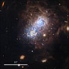 |
Fig. 1. Color-composite JWST image of I Zw 18 made using four near-IR NIRCam bands (F115W, F200W, F356W, and F444W) by ESA/Webb, NASA, CSA (Hirschauer et al. 2024). North is up, and east is left. The yellow circle represents the spectroscopic 1.5″ aperture of DESI. |
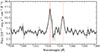 |
Fig. 2. Rest-frame DESI spectrum of I Zw 18 showing a clear detection of the [O II]λλ7320,7330 doublet. The gray shadowed area represents the error bars. The dashed vertical lines mark the position of the emission lines. |
Electron densities, [O III] temperatures t3, and element abundances in the I ZW 18 SE knot.
3. Determining the chemical abundances, electron densities, and temperatures
In this section, we describe the method we used to determine the electron densities (ne) and temperatures (Te) along with the chemical abundances. The calculations were performed using the code PyNeb in its version 1.1.24 (Luridiana et al. 2015) with the PyNeb atomic data dictionary PYNEB_23_01.
3.1. Extinction correction and electron density
The Balmer line ratios measured in the DESI spectrum of the SE knot deviate systematically from the theoretical Case B values, particularly for the higher-order Balmer lines. This cannot be explained by dust extinction alone. A more detailed analysis of the Balmer decrement, including the effect of stellar absorption, and suggested flux corrections are presented in Appendix A.
The spectral resolution of the DESI data enabled us to resolve the [O II]λλ3727,3729 doublet and the [S II]λλ6716,6731 doublet. For the I Zw 18 SE knot, we calculated line ratios of [O II]λ3729/[O II]λ3726 = 1.456±0.058 and [S II]λ6716/[S II]λ6731 = 1.473±0.066. From these diagnostic ratios, we found that the electron density ne from [O II]λ3729/[O II]λ3726 is equal to 27±32. The changes in ne are negligible for Te > 10 000 K, which is typical for extremely low-metallicity H II regions. Fig. 3 presents a comparison between the observed [O II] doublet flux ratio and theoretical ratios at varying ne. The figure demonstrates that the theoretical relation between ne and [O II]λ3729/[O II]λ3726 does not significantly depend on Te in the low-density regime. The[O II] doublet probes ne in the O+ ionization zone, for which we derive Te and the oxygen abundance below. Because the uncertainty in the ne estimation at low density is substantial, however, we did not use the computed ne value to determine Te and the chemical abundances. We instead assumed a fixed value of ne = 100 cm−3 because its effect is negligible in the calculation of the final ionic abundances at low density (Osterbrock & Ferland 2006). Nonetheless, we additionally verified our conclusion in the low-density regime using the [S II]λ6716/[S II]λ6731 ratio and found that the [S II] and [O II] doublets consistently show a low-density state (ne < 100 cm−3).
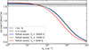 |
Fig. 3. [O II]λ3729/[O II]λ3726 ratio as a function of ne. The solid blue line represents the PyNeb model for Te = 20 000 K, which is typical for extremely low-metallicity H II regions. For comparison, the solid red line represents the PyNeb model for Te = 6000 K. The dotted line and gray area show the [O II]λ3729/[O II]λ3726 ratio derived from DESI spectrum and its uncertainty. |
3.2. Electron temperatures
From the combination of the nebular [O III]λλ4959,5007 and auroral [O III]λ4363 lines, we obtained Te([O III]) = 21 200 ± 860 K. This value is higher than the 19 600 ± 600 K that was reported for the SE knot by Kehrig et al. (2016) and than the averaged Te = 18 500 ± 2000 K that was measured across the entire galaxy by Rickards Vaught et al. (2025). These two studies both reported significant temperature variations (∼15 000–24 000 K) at galaxy scales and locally within its SE knot. Therefore, the slightly elevated value than the averaged estimates by previous IFS studies we obtained from the DESI spectrum is likely caused by the differences in the spatial sampling. Te(O II) was computed using the [O II]λλ3729,3726/[O II]λλ7320,7330 ratio and represents the lower ionization zone. It is significantly lower, Te([O II]) = 16 170±950 K.
As summarized by Méndez-Delgado et al. (2023), measurements of Te([O II]) can be variously affected by the uncertainty in the reddening correction or the quality of the flux calibration, the recombination contribution to the collisionally excited lines, temperature fluctuations, or density variations. We corrected the emission line fluxes to make them consistent with the theoretical Balmer decrement, however, and addressed potential issues with reddening and/or flux calibration. Possible temperature fluctuations within the O+ zone might lead to an overestimate of Te([O II]). This means that the average temperature in the O+ zone can be lower than Te([O II]) and should be considered as an upper limit. Possible density fluctuations will have similar effect. The [O II]λ3729/[O II]λ3726 and [S II]λ6716/[S II]λ6731 ratios indicate a low-density region in the two ionization zones. Although small high-density knots cannot be excluded, their contribution can only lower the average Te because a higher ne leads to a lower Te at a given [O II]λλ3729,3726/[O II]λλ7320,7330 ratio.
On the other hand, direct Te estimates in low-ionization zones at extremely low metallicities are crucial because there are indications that the relation between Te in zones of high and low ionization is nonlinear. Furthermore, the number of data points with simultaneous measurement of the two temperatures in the Te([O III]) > 14 000 K range is extremely limited (see, e.g., Arellano-Córdova & Rodríguez 2020; Méndez-Delgado et al. 2023), but it is very important to establish a reliable relation between Te([O III]) and Te([O II]) or Te([N II]) to accurately determine total oxygen abundance and the ICFs for abundances of other chemical elements, which sensitively depend on O+/O++.
It is interesting to compare our direct Te([O II]) estimate with the estimate obtained using popular t2 − t3 relations because they are widely used to calculate the metallicity of metal-poor galaxies when no auroral lines in low-ionization zones are available. The linear t2 − t3 relation by Garnett (1992) and our estimate of Te([O III]) gives Terel([O II]) = 17 840 ± 600 K, which is 16% higher than a direct estimate using the [O II]λλ7320,7330 lines. This result differs from the conclusion by Méndez-Delgado et al. (2023), who found that Te([N II]) at high temperature is significantly lower than predicted by linear relations, similar to Garnett (1992). Although the maximum Te([O III]) in the sampel of Méndez-Delgado et al. (2023) was limited to ∼14 000 K, we extend the range to 21200 K with our measurement. The measured Te([O II]) in I Zw 18 is also relevant for high-redshift SF galaxies, which typically exhibit high ionization parameters and a low metallicity. Some previous studies have shown that the t2 − t3 relation may depend on the ionization parameter (e.g. Pilyugin 2007; Arellano-Córdova & Rodríguez 2020). In this context, I Zw 18 serves as a local analog of high-z systems. As shown in Fig. 4, our temperature measurements for I Zw 18 are most consistent with the t2 − t3 relations by Cataldi et al. (2025), which were developed considering high-redshift objects, and with Pagel et al. (1992) based on photoionization models. This indicates that t2 − t3 relations at high temperatures might be more complex than a one-dimensional relation, and it highlights the need for further studies of the temperature structure at low metallicities.
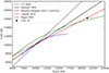 |
Fig. 4. Te([O II]) as a function of Te([O III]) for the model from Garnett (1992) (solid black line) in comparison with Te([O II]) and Te([O III]) derived for the SE knot in I Zw 18 (black circle). The solid blue line represents the quadratic model from Méndez-Delgado et al. (2023) for Te([N II]) as a function of Te([O III]), and the red and green lines represent the relations from Cataldi et al. (2025) and Pagel et al. (1992), respectively. For this model, we preserved a limited range of Te([O III]), which represents the range of Te([O III]) in its calibration sample. |
The detection of the [S III]λ6312 line enabled us to calculate Te in the medium-temperature [S III] zone, Te([S III]), because the [S III]λ9531/[S III]λ9069 ratio differs substantially from 2.47, which is the theoretical value. This may indicate telluric absorptions in the [S III]λ9069 line. We therefore only used the [S III]λ9531 nebular line to compute Te([S III]). We determined Te([S III]) = 17290±1750 K, which falls between Te([O II]) and Te([O III]).
3.3. Chemical abundances
Because we derived Te directly from the auroral to nebular line ratios in the [O II] and [O III] zones, we estimated the total oxygen abundance using these Te([O II]) and Te([O II]) values together with the fluxes of [O II]λλ3729,3726 and [O III]λλ4959,5007 assuming a low-density regime. A negligible ionic O3+ abundance is expected because the He IIλ4686 line is not detected in the spectrum. Applying the PyNeb getIonAbundance method and combining O+ and O++ abundances, we obtained 12+log(O/H) = 7.066 ± 0.046.
Since in previous studies neither the [O II] nor the [N II] auroral lines were measured, the authors relied on the t2 − t3 relations to estimate O/H. Therefore, we also estimated O/H by computing Te([O II]) from Te([O III]) using the t2 − t3 relation from Garnett (1992). In this case, we obtained 12+log(O/H)t2t3 = 7.036 ± 0.035, which is compatible with our estimate using direct measurements of both Te([O II]) and Te([O II]). The alternative quadratic t2 − t3 relation from Méndez-Delgado et al. (2023) only extends to 17 000 K and can therefore not be applied to I Zw 18 without significant extrapolation. Recently, Rickards Vaught et al. (2025) applied three- and two-state models and a parametric t2 − t3 relation dependent on the excitation parameter and found an oxygen abundance of 7.2 ± 0.02 dex, which is higher by 0.15 dex than our estimate. Thus, different t2 − t3 relations provide varying estimates of the total O/H, which highlights the need for further studies to better constrain these relations and Te([O II]) for low-metallicity galaxies.
Assuming N/O ∼ N+/O+ and Te([O II]) ∼Te([N II]), we obtained the nitrogen-to-oxygen ratio log(N/O) = –1.509 ± 0.097, which is consistent with average value for metal-poor galaxies from Zinchenko et al. (2024). Using the method described by Zinchenko et al. (2024), we also derived log(S/O) = −1.558 ± 0.041. This value is very close to the average S/O ratio for metal-poor galaxies as reported by Zinchenko et al. (2024).
4. Conclusions
We presented the first direct measurement of the electron temperature in the low-ionization zone of I Zw 18, enabled by the detection of the [O II]λλ7320,7330 auroral doublet in the DESI DR1 spectrum. We found a substantial temperature difference between the ionization zones, with Te([O III]) = 21 200 ± 860 K exceeding Te([O II]) = 16170 ± 950 K. This Te([O II]) value lies between the t2 − t3 relations proposed by Garnett (1992) and Méndez-Delgado et al. (2023) and provides the first direct Te([O II]) estimate for very high temperatures. It is far beyond Te([O III]) ∼ 17 000 K, where no empirical t2 − t3 are calibrated. Using direct temperature measurements for the two ionization zones, we derived 12+log(O/H) = 7.066 ± 0.046. We also derived log(N/O) = –1.509 ± 0.097 and log(S/O) = –1.558 ± 0.041, which are consistent with the average values for metal-poor galaxies from Zinchenko et al. (2024).
Our results extend the calibration of Te relations to the highest temperatures and provide important anchor points for the temperature structure of extremely metal-poor H II regions. The potential systematic biases in the metallicities derived using empirical or theoretical temperature relations might have important implications for studies of metal-poor galaxies (e.g., the derivation of the primordial helium abundance), including high-redshift galaxies, where direct Te measurements in [O II] zone are mostly impossible, and the abundance estimates rely on these relations. Accurate chemical abundance determinations in primordial environments therefore require direct Te measurements in all ionization zones or robust t2 − t3 relations. This highlights the need for improved models of temperature structures in extremely metal-poor galaxies.
Acknowledgments
We are grateful to the referee for his or her constructive comments. IAZ acknowledges funding from the Deutsche Forschungsgemeinschaft (DFG; German Research Foundation)–project-ID 550945879. JVM acknowledge financial support from the Spanish MINECO grant PID2022-136598NB-C32 and from the AEI “Center of Excellence Severo Ochoa” award to the IAA (SEV-2017-0709). PP acknowledges support by Fundação para a Ciência e a Tecnologia (FCT) grants UID/FIS/04434/2019, UIDB/04434/2020, UIDP/04434/2020 and Principal Investigator contract CIAAUP-092023-CTTI. JEM-D thanks the support of the SECIHTI CBF-2025-I-2048 project “Resolving the Internal Physics of Galaxies: From Local Scales to Global Structure with the SDSS-V Local Volume Mapper” (PI: Méndez-Delgado). This research used data obtained with the Dark Energy Spectroscopic Instrument (DESI). DESI construction and operations are managed by the Lawrence Berkeley National Laboratory. This material is based upon work supported by the U.S. Department of Energy, Office of Science, Office of High-Energy Physics, under Contract No. DE–AC02–05CH11231, and by the National Energy Research Scientific Computing Center, a DOE Office of Science User Facility under the same contract. Additional support for DESI was provided by the U.S. National Science Foundation (NSF), Division of Astronomical Sciences under Contract No. AST-0950945 to the NSF’s National Optical-Infrared Astronomy Research Laboratory; the Science and Technology Facilities Council of the United Kingdom; the Gordon and Betty Moore Foundation; the Heising-Simons Foundation; the French Alternative Energies and Atomic Energy Commission (CEA); the National Council of Science and Technology of Mexico (CONACYT); the Ministry of Science and Innovation of Spain (MICINN), and by the DESI Member Institutions: www.desi.lbl.gov/collaborating-institutions.
References
- Arellano-Córdova, K. Z., & Rodríguez, M. 2020, MNRAS, 497, 672 [CrossRef] [Google Scholar]
- Cataldi, E., Belfiore, F., Curti, M., et al. 2025, A&A, 703, A208 [NASA ADS] [CrossRef] [EDP Sciences] [Google Scholar]
- Croxall, K. V., Pogge, R. W., Berg, D. A., Skillman, E. D., & Moustakas, J. 2016, ApJ, 830, 4 [NASA ADS] [CrossRef] [Google Scholar]
- DESI Collaboration (Abdul-Karim, M., et al.) 2025, ArXiv e-prints [arXiv:2503.14745] [Google Scholar]
- Fiorentino, G., Contreras Ramos, R., Clementini, G., et al. 2010, ApJ, 711, 808 [CrossRef] [Google Scholar]
- Fitzpatrick, E. L. 1999, PASP, 111, 63 [Google Scholar]
- Flury, S. R., Jaskot, A. E., Ferguson, H. C., et al. 2022, ApJ, 930, 126 [NASA ADS] [CrossRef] [Google Scholar]
- Garnett, D. R. 1992, AJ, 103, 1330 [NASA ADS] [CrossRef] [Google Scholar]
- Hirschauer, A. S., Crouzet, N., Habel, N., et al. 2024, AJ, 168, 23 [NASA ADS] [CrossRef] [Google Scholar]
- Izotov, Y. I., & Thuan, T. X. 1998, ApJ, 497, 227 [Google Scholar]
- Izotov, Y. I., Thuan, T. X., & Lipovetsky, V. A. 1994, ApJ, 435, 647 [NASA ADS] [CrossRef] [Google Scholar]
- Izotov, Y. I., Stasińska, G., Meynet, G., Guseva, N. G., & Thuan, T. X. 2006, A&A, 448, 955 [CrossRef] [EDP Sciences] [Google Scholar]
- Kehrig, C., Vílchez, J. M., Pérez-Montero, E., et al. 2016, MNRAS, 459, 2992 [NASA ADS] [CrossRef] [Google Scholar]
- Luridiana, V., Morisset, C., & Shaw, R. A. 2015, A&A, 573, A42 [NASA ADS] [CrossRef] [EDP Sciences] [Google Scholar]
- Méndez-Delgado, J. E., Esteban, C., García-Rojas, J., et al. 2023, MNRAS, 523, 2952 [CrossRef] [Google Scholar]
- Moustakas, J., Scholte, D., Dey, B., & Khederlarian, A. 2023, Astrophysics Source Code Library [record ascl:2308.005] [Google Scholar]
- Osterbrock, D. E., & Ferland, G. J. 2006, Astrophysics of gaseous nebulae and active galactic nuclei [Google Scholar]
- Pagel, B. E. J., Simonson, E. A., Terlevich, R. J., & Edmunds, M. G. 1992, MNRAS, 255, 325 [CrossRef] [Google Scholar]
- Pérez-Montero, E. 2017, PASP, 129, 043001 [CrossRef] [Google Scholar]
- Pérez-Montero, E., & Díaz, A. I. 2003, MNRAS, 346, 105 [CrossRef] [Google Scholar]
- Pilyugin, L. S. 2007, MNRAS, 375, 685 [Google Scholar]
- Rickards Vaught, R. J., Hunt, L. K., Aloisi, A., et al. 2025, ApJ, 990, 111 [Google Scholar]
- Scarlata, C., Hayes, M., Panagia, N., et al. 2024, ArXiv e-prints [arXiv:2404.09015] [Google Scholar]
- Skillman, E. D., & Kennicutt, R. C., Jr 1993, ApJ, 411, 655 [NASA ADS] [CrossRef] [Google Scholar]
- Stasińska, G. 1980, A&A, 85, 359 [Google Scholar]
- Ucci, G., Ferrara, A., Gallerani, S., et al. 2019, MNRAS, 483, 1295 [NASA ADS] [CrossRef] [Google Scholar]
- Vílchez, J. M., & Iglesias-Páramo, J. 1998, ApJ, 508, 248 [CrossRef] [Google Scholar]
- Yates, R. M., Schady, P., Chen, T. W., Schweyer, T., & Wiseman, P. 2020, A&A, 634, A107 [NASA ADS] [CrossRef] [EDP Sciences] [Google Scholar]
- Zinchenko, I. A., Sobolenko, M., Vílchez, J. M., & Kehrig, C. 2024, A&A, 690, A28 [NASA ADS] [CrossRef] [EDP Sciences] [Google Scholar]
- Zurita, A., Florido, E., Bresolin, F., Pérez, I., & Pérez-Montero, E. 2021, MNRAS, 500, 2380 [Google Scholar]
Appendix A: Emission line fluxes and correction for extinction
We summarize emission line measurements from the VAC FASTSPECFIT catalog in Table A.1. The fluxes returned by FASTSPECFIT are already corrected for Galactic extinction. This table shows that the measured Hα/Hβ ratio (2.649 ± 0.020) is ≃3% lower than the theoretical value expected at Te = 20 000 K, formally yielding a negative c(Hβ) = − 0.045 ± 0.009 when applying the extinction curve of Fitzpatrick (1999), while previous studies reported a small positive c(Hβ) values (Skillman & Kennicutt 1993; Vílchez & Iglesias-Páramo 1998; Izotov et al. 1994; Kehrig et al. 2016). Ucci et al. (2019) using the same IFU data as Kehrig et al. (2016), also reported very low but positive visual extinction values, AV ∼ 0.01 mag, in most spaxels.
Emission line fluxes normalized to Hβ = 100.
At the same time, the observed Hγ/Hβ and Hδ/Hβ ratios exceed their theoretical values by ∼6–12%, also implying negative c(Hβ). For the physical conditions typical of metal-poor H II regions, we adopt Case B Balmer ratios at ne = 100 cm−3 and Te = 20 000 K computed with PYNEB. The theoretical ratios used in this work are listed in Table A.1. These Balmer ratios therefore cannot be explained by a physically plausible dust extinction correction alone.
To test whether overestimation of absorption features during stellar continuum modelling can explain these discrepancies, we refit all Balmer emission lines using single-Gaussian profiles without subtracting stellar component. While this brings Hα/Hβ closer to the theoretical ratio, it does not significantly change Hγ/Hβ or Hδ/Hβ, which remain discrepant beyond their uncertainties as shown in Figure A.1. Thus, we conclude that the elevated higher-order Balmer ratios are not caused by the stellar population fitting performed by FASTSPECFIT.
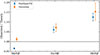 |
Fig. A.1. Observed-to-theoretical Balmer line ratios (Hα/Hβ, Hγ/Hβ, Hδ/Hβ) for two measurement methods. Blue circles represent full spectral fitting including stellar absorption component from FASTSPECFIT catalog. Orange squares represent our fitting with single Gaussian without subtraction of stellar continuum. Error bars show 1σ uncertainties, and the dashed line marks the consistency with Case B recombination at ne = 100 cm−3 and Te = 20 000 K. |
Thus, we consider a relative flux calibration bias in the blue part of the DESI spectrum as a likely scenario. Although, we cannot rule out possible deviations from the standard Case B assumptions at very high Te (e.g. Flury et al. 2022; Scarlata et al. 2024). We therefore apply an empirical correction to the blue spectral region, derived from the ratios of the observed to theoretical Hγ/Hβ and Hδ/Hβ values. The resulting correction factors correspond to a reduction of the measured fluxes by ∼12% for [O II]λλ3726, 3729 and ∼10% for [O III]λ4363, based on their proximity in wavelength to the relevant Balmer lines.
Applying this correction increases the derived Te(O II), but lowers Te(O III), bringing our Te(O III) estimate for the SE knot into closer agreement with previous IFU-based studies (e.g. Kehrig et al. 2016; Rickards Vaught et al. 2025). Increase of [O II]λλ3726, 3729 flux by 10% in Te(O II) range of 14 000–16 000 K results in Te(O II) uncertainty of 1 000–1 200 K, which is compatible with statistical uncertainty of our Te(O II) estimation. Figure A.2 demonstrates the effect of a systematic increase in the [O II]λλ3726, 3729 flux on the derived electron temperature. In this toy model the Te([O II]) is computed using PyNeb over a range of input ratios [O II] nebular-to-auroral line ratios (25–250). The x-axis shows the Te for the reference case, while the y-axis shows the temperature difference ΔTe between the reference case and a 10% increase in [O II]λλ3726, 3729 flux.
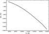 |
Fig. A.2. Difference in the derived Te([O II]) caused by a 10% increase in the [O II]λλ3726,3729 flux as a function of the original temperature. |
All Tables
Electron densities, [O III] temperatures t3, and element abundances in the I ZW 18 SE knot.
All Figures
|
Fig. 1. Color-composite JWST image of I Zw 18 made using four near-IR NIRCam bands (F115W, F200W, F356W, and F444W) by ESA/Webb, NASA, CSA (Hirschauer et al. 2024). North is up, and east is left. The yellow circle represents the spectroscopic 1.5″ aperture of DESI. |
| In the text | |
|
Fig. 2. Rest-frame DESI spectrum of I Zw 18 showing a clear detection of the [O II]λλ7320,7330 doublet. The gray shadowed area represents the error bars. The dashed vertical lines mark the position of the emission lines. |
| In the text | |
|
Fig. 3. [O II]λ3729/[O II]λ3726 ratio as a function of ne. The solid blue line represents the PyNeb model for Te = 20 000 K, which is typical for extremely low-metallicity H II regions. For comparison, the solid red line represents the PyNeb model for Te = 6000 K. The dotted line and gray area show the [O II]λ3729/[O II]λ3726 ratio derived from DESI spectrum and its uncertainty. |
| In the text | |
|
Fig. 4. Te([O II]) as a function of Te([O III]) for the model from Garnett (1992) (solid black line) in comparison with Te([O II]) and Te([O III]) derived for the SE knot in I Zw 18 (black circle). The solid blue line represents the quadratic model from Méndez-Delgado et al. (2023) for Te([N II]) as a function of Te([O III]), and the red and green lines represent the relations from Cataldi et al. (2025) and Pagel et al. (1992), respectively. For this model, we preserved a limited range of Te([O III]), which represents the range of Te([O III]) in its calibration sample. |
| In the text | |
|
Fig. A.1. Observed-to-theoretical Balmer line ratios (Hα/Hβ, Hγ/Hβ, Hδ/Hβ) for two measurement methods. Blue circles represent full spectral fitting including stellar absorption component from FASTSPECFIT catalog. Orange squares represent our fitting with single Gaussian without subtraction of stellar continuum. Error bars show 1σ uncertainties, and the dashed line marks the consistency with Case B recombination at ne = 100 cm−3 and Te = 20 000 K. |
| In the text | |
|
Fig. A.2. Difference in the derived Te([O II]) caused by a 10% increase in the [O II]λλ3726,3729 flux as a function of the original temperature. |
| In the text | |
Current usage metrics show cumulative count of Article Views (full-text article views including HTML views, PDF and ePub downloads, according to the available data) and Abstracts Views on Vision4Press platform.
Data correspond to usage on the plateform after 2015. The current usage metrics is available 48-96 hours after online publication and is updated daily on week days.
Initial download of the metrics may take a while.