| Issue |
A&A
Volume 706, February 2026
|
|
|---|---|---|
| Article Number | L3 | |
| Number of page(s) | 6 | |
| Section | Letters to the Editor | |
| DOI | https://doi.org/10.1051/0004-6361/202558202 | |
| Published online | 27 January 2026 | |
Letter to the Editor
Quiet, but not silent
The X-ray activity of the Maunder minimum star HD 166620
1
Institut für Astronomie und Astrophysik, Eberhard Karls Universität Tübingen Sand 1 72076 Tübingen, Germany
2
501 Campbell Hall, University of California at Berkeley Berkeley CA 94720, USA
3
Max-Planck-Institut für extraterrestrische Physik Giessenbachstrasse 1 85748 Garching, Germany
★ Corresponding author: This email address is being protected from spambots. You need JavaScript enabled to view it.
Received:
21
November
2025
Accepted:
26
December
2025
Abstract
As the only known unambiguous star in a Maunder minimum-like chromospheric activity state, the properties of HD 166620 can provide valuable insight into the behaviour of the Sun during the historic extended low-states of its activity cycle. The coronal X-ray activity of HD 166620 has so far only been probed with a ROSAT/HRI observation in 1996, near the chromospheric activity maximum before the star entered its grand minimum around 2004. We conducted a deep XMM-Newton observation of HD 166620 during its chromospheric Ca II H&K activity grand minimum to achieve a better understanding of its magnetic activity. We detected HD 166620 with an X-ray luminosity of log LX(erg s−1) = 26.56+0.10−0.12, corresponding to log(LX/Lbol = −6.58+0.10−0.12 and an X-ray surface flux of log FX(erg s−2 s−1 = 3.97+0.10−0.12. With respect to the earlier ROSAT observation, the X-ray brightness of HD 166620 has decreased by a factor of 2.5 during its Maunder minimum-like state. To place its X-ray properties into context, we constructed an X-ray sample of late-type stars within 10 pc of the Sun. The activity of HD 166620 is below the levels of all other K dwarfs in the 10 pc sample. The corona of HD 166620 during its grand minimum emits at the level of the solar background corona, which implies that it has no large active magnetic structures. Along with long-term Ca II H&K monitoring of HD 166620, this result provides evidence that the solar activity during the Maunder minimum was not reduced significantly below the levels seen during its present-day cycle minima. The similar X-ray surface flux of HD 166620 and the modern quiet Sun, and also their Rossby number near the critical value of spin-down models, suggest a connection between the regime of weakened magnetic braking and the occurrence of Maunder minimum states.
Key words: Sun: activity / stars: activity / stars: coronae / stars: individual: HD 166620 / X-rays: stars
© The Authors 2026
 Open Access article, published by EDP Sciences, under the terms of the Creative Commons Attribution License (https://creativecommons.org/licenses/by/4.0), which permits unrestricted use, distribution, and reproduction in any medium, provided the original work is properly cited.
This article is published in open access under the Subscribe to Open model. This email address is being protected from spambots. You need JavaScript enabled to view it. to support open access publication.
1. Introduction
During the solar Maunder minimum (henceforth MM) between 1645–1715, historical records show an extended period with significantly decreased sunspot counts and auroral sightings (Usoskin et al. 2015). The cause for this extended low-activity state is still unknown and might have profound implications for our understanding of the underlying mechanisms of stellar dynamos and its effects on the climates of Earth and exoplanets. Furthermore, it is still to be determined whether the solar magnetic field during the MM was extremely weak or if it was near the cycle-minimum amplitude (Baum et al. 2022).
In order to constrain stellar properties during MM states, it is crucial to confirm their occurrence in other Sun-like stars. The systematic search for extrasolar activity cycles began with the Mount Wilson HK survey (Baliunas et al. 1995), in which chromospheric Ca II H&K lines of 111 stars with spectral types (SpT) F to M were monitored for three decades. The ratio of the fluxes of the H- and K-emission lines and the continuum on either side defines the SHK-index, which is widely used to characterise chromospheric activity (Vaughan et al. 1978). The Mount Wilson survey revealed a high number of “flat” stars with a low and constant SHK-index (Baliunas et al. 1995). Initially flagged as potential MM-like states, most of these targets were instead found in their post-main-sequence subgiant phase, which suggests that MM states might be much rarer than was assumed before (Wright 2004).
To date, only a few MM candidates have been identified. Due to declining magnetic activity, HD 4915 was proposed as an MM candidate by Shah et al. (2018), but this was refuted by Flores Trivigno et al. (2024) based on further monitoring. Other reported candidates are HD 217014 (Poppenhäger et al. 2009), HD 20807 (Flores et al. 2021), and TIC 352227373 & TYC 7560-477-1 (Järvinen & Strassmeier 2025). Whether these stars are in an MM or are generally inactive remains inconclusive, however. The only known star that unambiguously is in an MM-like state is HD 166620. Five decades of data from long-term SHK-index monitoring clearly show that its pronounced activity cycle stopped (Baum et al. 2022; Luhn et al. 2022).
We provide the first X-ray detection of the K2 dwarf HD 166620 since the start of its reduced chromospheric activity approximately 20 years ago. For this purpose, we conducted a dedicated observation with XMM-Newton. We determine the X-ray surface flux of HD 166620 and compare it with the surface fluxes of different types of magnetic structures seen on the Sun. To place the observed activity level of HD 166620 into context, we construct an X-ray sample of all FGK dwarfs within 10 pc based on the work of Reylé et al. (2021). In Sect. 2 we describe the SHK and X-ray data and analysis for HD 166620 and the 10 pc sample. We present and discuss the results of our analysis in Sect. 3, and we summarise our findings in Sect. 4.
2. Data and analysis
2.1. SHK activity
Long-term measurements of the SHK activity of HD 166620 have been discussed by Luhn et al. (2022), who used Mount Wilson and Keck/HIRES data from Baum et al. (2022) and Oláh et al. (2016). Since then, more Keck/HIRES data were published by Isaacson et al. (2024). For the time of our XMM-Newton observation (which is described in Sect. 2.2), we obtained data from the monitoring program of the Lick Automated Planet Finder (APF) (Vogt et al. 2014). We discuss the APF data in Appendix A.
The complete SHK-index time series of HD 166620 is presented in Fig. 1. We binned the data in 120 d steps and fitted the two observed cycle maxima with Gaussian functions. The Gaussians were not meant to represent a physical model of the variability and were only used to determine the time of the maxima. The peaks of the two Gaussians are separated by 15.5 years, which agrees with the cycle period of 15.8 ± 0.3 years found by Baliunas et al. (1995). Extrapolation predicts the subsequent maxima to occur in late-2010 and mid-2026, potentially with a trend of decreasing peak SHK values, as indicated by the dashed blue line in Fig. 1. No activity increase is visible in the SHK data after the decrease from the 1995 maximum, however. Our new data from the APF still show no systematically increased activity, even though they were acquired only approximately one year before the predicted 2026 maximum. During the extended low state, the SHK level is similar to the pre-MM cycle minima.
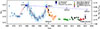 |
Fig. 1. SHK and RX time series for HD 166620 with data compiled by Luhn et al. (2022) and more recent data from Keck/HIRES (Isaacson et al. 2024) and the APF (Vogt et al. 2014). The small transparent symbols mark individual SHK measurements, and the larger opaque symbols are the same data, binned in 120 d bins. A black outline denotes a bin containing only a single measurement. The dashed blue line shows the extrapolated trend of the two maxima (see Sect. 2.1). The two X-ray measurements are overplotted with black squares, and their epochs are marked on the axis. |
2.2. X-ray activity
The only X-ray detection of HD 166620 to date is from a ROSAT/HRI observation on 26 October 1996 (Schmitt & Liefke 2004), shortly after the last maximum of its SHK cycle. We conducted a dedicated XMM-Newton observation on 10 March 2025 to quantify the X-ray activity level during its MM-like state.
For the data analysis, we used the XMM-Newton Science Analysis Software (SAS) version 22.0.0. Given the low X-ray brightness of HD 166620, we only considered the data from the most sensitive XMM-Newton instrument, EPIC/pn. To eliminate effects of solar background irradiation, we filtered out time intervals with high-energy (≥10 keV) count rates on the whole detector above 0.3 ct/s, which left a net total observation time of 28.9 ks. Additionally, we excluded bad pixels (flag = 0) and retained events with pattern ≤4. We ran the source detection, and the number of net source counts is 87.4 ± 12.9 for the full 0.2–12.0 keV energy band of EPIC/pn.
We extracted a spectrum and the corresponding response files from a source region with a radius of 30″ centred on the position of HD 166620 at the epoch of the observation, which matches the position from the source detection within 0.1″. The region we used for background-subtraction has a radius of 50″ and is located on the same CCD. Then, we performed the spectral analysis with XSPEC1 version 12.14.1 using a spectral binning of ≥15 counts. We fitted a two-temperature thermal model (APEC, Smith et al. 2001). Using the library from Asplund et al. (2009), we set the global abundance of the stellar corona to a typical value of Z = 0.3 Z⊙ (see e.g. Robrade & Schmitt 2005; Maggio et al. 2007), leaving the coronal plasma temperatures and the emission measures of the two components free to be fit. At the lower end, the energy range considered for the fit was limited to ≥0.2 keV because the calibration of EPIC is unreliable at lower energies. At the upper end, we limited the spectrum to ≤5.0 keV because the count rate of HD 166620 is low at higher energies. The best-fit model yields a coronal plasma temperature of  for the cooler component. While the low number of counts prevented us from constraining temperature of the hotter component well, a statistically significant improvement over a one-temperature model is visible. The Fisher test (Fisher 1922) yielded a p-value corresponding to a significance of 3.28σ. The spectrum and best-fit model are presented in Fig. 2. The hotter component of the two-temperature model only contributes ≈10% of the total emission measure and thus has a small effect on the total flux. We discuss the hardness ratios in Appendix B. In the ROSAT energy band of 0.1–2.4 keV, convolution of the spectral model with the cflux component yields a flux of
  .
.
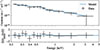 |
Fig. 2. Top: XMM-Newton EPIC/pn spectrum of HD 166620 and best-fit 2T-APEC thermal model. Bottom: Residuals. |
For both X-ray detections, we used the HD166620 Gaia DR3 parallax of ϖ = 90.1234 mas (Gaia Collaboration 2023) to calculate the X-ray luminosity LX. The bolometric luminosity of log Lbol(L⊙) = −0.45 ± 0.02 and a radius of R* = 0.80 ± 0.02 R⊙ (Brewer et al. 2016) were used to derive RX = LX/Lbol and the X-ray surface flux FX. The values for these X-ray activity diagnostics are presented in Table 1, and Rx is overlaid on the SHK time series in Fig. 1. The X-ray activity level of HD 166620 has decreased by a factor of 2.5 from its value close to the peak of the pre-MM chromospheric cycle to its present MM-like state.
X-ray properties of HD 166620.
2.3. Comparison sample
For comparison, we refer to the M10 pc sample described by Caramazza et al. (2023). Following a similar methodological approach, we compiled a sample of all FGK-type dwarfs within 10 pc from the Sun (henceforth FGK 10 pc) based on the work of Reylé et al. (2021) and the SpT therein (Bennedik et al., in prep.). The FGK 10 pc sample includes 64 stars, 56 of which have reliable Gaia photometry. We collected X-ray data from ROSAT, eROSITA, and XMM-Newton observations. To achieve this, we made use of the Second ROSAT All-Sky Survey Point Source Catalogue (2RXS) (Boller et al. 2016), the Second ROSAT Source Catalogue of Pointed Observations (2RXP) (ROSAT Consortium 2000), the eROSITA DR1 catalogue (Merloni et al. 2024), and EPIC/pn detections in the 4XMM-DR14 catalogue (Webb et al. 2020). In total, the FGK 10 pc sample contains X-ray data for 61 stars, resulting in a completeness of > 95%. Within this sample, 4 stars are marked as subgiants by Reylé et al. (2021), which we excluded from the analysis. The count rates listed in the X-ray catalogues were converted into a flux in the 0.1–2.4 keV ROSAT energy band with proper conversion factors that depended on the instrumental setup (see Appendix C). With the parallaxes given by Reylé et al. (2021), we computed LX.
As discussed in Appendix D, we used isochrones from the PARSEC V2.0 database (Nguyen et al. 2022, 2025) to estimate the bolometric luminosities and effective temperatures and the Stefan-Boltzmann law to determine the stellar radii. Finally, we computed RX and FX values for the FGK 10 pc sample.
3. Discussion
Our systematic assessment of the stellar parameters and X-ray brightness of the FGK 10 pc sample allowed us to place the activity of HD 166620 into context. In Fig. 3 we show the mean observed RX values for each star in the FGK 10 pc sample and the M10 pc sample from Caramazza et al. (2023). We display values for the X-ray observations of HD 166620 and the solar ROSAT-band X-ray luminosities during its cycle extrema of  by Peres et al. (2000).
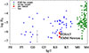 |
Fig. 3. X-ray over bolometric luminosity for HD 166620 in its two detections compared with the range of values observed throughout the solar cycle (Peres et al. 2000) and for FGK (Bennedik et al., in prep.) and M0–M4 dwarfs (Caramazza et al. 2023) within 10 pc of the Sun. |
Fig. 3 shows that the X-ray emission of FGK dwarfs spans at least three orders of magnitude. This was known from previous systematic studies such as Schmitt & Liefke (2004), who used a smaller sample in the ROSAT era, and Zhu & Preibisch (2025), who presented a compilation of X-ray data for a larger but less complete sample of GKM stars. The ROSAT detection places HD 166620 at the lower end of the observed RX range of K dwarfs, even though this measurement was taken close to the maximum of its chromospheric cycle. After the onset of the MM-like state, the RX value of HD 166620 has dropped below that seen in all other K dwarfs within the 10 pc sample. The rising slope of the lower envelope in Fig. 3 is likely due to the longer spin-down timescales of later-type stars, which delay their development to low activity levels (Preibisch et al. 2005; Johnstone et al. 2021). Thus, the position of HD 166620 at the low activity end is in line with its slow rotation (45 d, Luhn et al. 2022) and old age ( , Brewer et al. 2016).
The X-ray surface flux, FX, is a parameter that offers the possibility to directly compare stellar and solar activity levels since it is independent of the size of the emitting region. Extending Fig. 3 of Caramazza et al. (2023), we show in Fig. 4 the FX of HD 166620, the stars in the FGK 10 pc sample, and the M10 pc sample together with the typical values of different types of solar coronal magnetic structures. The latter, divided into solar coronal holes (CH), background corona (BKC), active regions (AR), and cores of active regions (CO), were derived from data from the Yohkoh satellite, originally as part of the Sun as an X-ray star project (Orlando et al. 2001, 2004), and their FX values were presented by Caramazza et al. (2023).
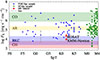 |
Fig. 4. Same as Fig. 3, but for X-ray surface fluxes FX. The typical ranges of FX exhibited by different types of solar coronal structures (from Caramazza et al. 2023) are depicted as coloured stripes. |
While at the time of the ROSAT observation, the FX of HD 166620 was at the upper edge of the values exhibited by solar BKC, during its current MM-like state, the HD 166620 corona is fully consistent with the emission levels of solar BKC and just slightly above the upper boundary for CH. The solar BKC consists of quiet magnetic loops that trap relatively low-temperature (≈1 MK) plasma (Orlando et al. 2001; Reale 2014). The X-ray plasma temperature of 0.1 keV derived from the XMM-Newton spectrum of HD 166620 is coincident with this value, which further strengthens the hypothesis that during its current MM state, the star resembles the quiet Sun. The surface-averaged X-ray flux of the Sun itself (Peres et al. 2000) is in the range of the BKC throughout the low-activity part of its 11-year cycle. Full-disk images from solar instruments such as Yohkoh or Hinode show the absence of high-activity magnetic structures such as CO and flares during solar minima (Adithya et al. 2021).
When HD 166620 is considered as a template for the Sun, our results provide evidence that the solar activity level during the historical MM was not reduced far below the level seen during its modern-time cycle minima. This agrees with direct coronal observations of solar eclipses in the historical MM, which show a weak and unstructured corona. If the Sun had been covered with large magnetic structures, it is likely that these would have been seen in reports and paintings at the time (see Hayakawa et al. (2021), Usoskin et al. (2015) for such historical observations).
The 10 pc sample shows that HD 166620 during its MM state and the Sun during its cycle minimum appear to define a natural lower boundary of the surface-averaged coronal X-ray flux; with the exception of very rare coronal-hole stars (Caramazza et al. 2023). This flux is provided by the small quiet magnetic loops of the solar(-like) BKC on both stars. Despite its later SpT, HD 166620 is a close analogue of the Sun in terms of its large-scale magnetic field as well. Specifically, both stars are located at the critical Rossby number that identifies stars with weak dipolar field due to low dynamo efficiency (Metcalfe et al. 2025). In simulations of the Babcock-Leighton dynamo, slowly rotating stars produce magnetic cycles with long-term variations of the strength of the dipole, and the low dynamo number of these stars makes their recovery from phases of a weak cycle slow, which in turn leads to grand minima (Vashishth et al. 2023). Other stars with a similar BKC-like X-ray surface flux as HD 166620 and the Sun can therefore be expected to undergo MM states. These stars can be identified as the objects in the weakened magnetic braking regime (van Saders et al. 2016; Metcalfe et al. 2025).
4. Summary and conclusions
The K2 dwarf HD 166620 is the only star that is unambiguously known to be in an MM-like activity state. Our XMM-Newton observation is the first X-ray detection since the onset of its diminished activity in approximately 2004. In its current MM-like state, the X-ray emission of HD 166620 has decreased by a factor of 2.5 compared to its pre-MM state, and it lies at 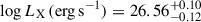 and
and 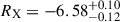 . This is slightly below the lower envelope defined by the other K dwarfs within 10 pc. The X-ray surface flux of HD 166620,
  , is consistent with the emission levels typically seen in the solar background corona, which dominates the minimum of the solar cycle. Together with the SHK time series of HD 166620, this suggests that during the MM of the Sun, the magnetic activity was not reduced significantly below the levels seen during its current cycle minima.
Acknowledgments
We thank the anonymous referee for their feedback and suggestions. MB and MC acknowledge support by the Bundesministerium für Wirtschaft und Energie through the Deutsches Zentrum für Luft- und Raumfahrt (DLR) under grant numbers FKZ 50 OR 2505 and FKZ 50 OR 2316. This research has made use of data obtained from the 4XMM XMM-Newton serendipitous source catalogue compiled by the 10 institutes of the XMM-Newton Survey Science Centre selected by ESA, and of archival data of the ROSAT space mission. This work is also based on data from eROSITA, the soft X-ray instrument aboard SRG, a joint Russian-German science mission supported by the Russian Space Agency (Roskosmos), in the interests of the Russian Academy of Sciences represented by its Space Research Institute (IKI), and the DLR. The SRG spacecraft was built by Lavochkin Association (NPOL) and its subcontractors, and is operated by NPOL with support from the Max Planck Institute for Extraterrestrial Physics (MPE). The development and construction of the eROSITA X-ray instrument was led by MPE, with contributions from the Dr. Karl Remeis Observatory Bamberg & ECAP (FAU Erlangen-Nuernberg), the University of Hamburg Observatory, the Leibniz Institute for Astrophysics Potsdam (AIP), and the Institute for Astronomy and Astrophysics of the University of Tübingen, with the support of DLR and the Max Planck Society. The Argelander Institute for Astronomy of the University of Bonn and the Ludwig Maximilians Universität Munich also participated in the science preparation for eROSITA. This research has made use of data and software provided by the High Energy Astrophysics Science Archive Research Center (HEASARC), which is a service of the Astrophysics Science Division at NASA/GSFC. This work has made use of data from the ESA mission Gaia (https://www.cosmos.esa.int/gaia), processed by the Gaia Data Processing and Analysis Consortium (DPAC, www.cosmos.esa.int/web/gaia/dpac/consortium). Funding for the DPAC has been provided by national institutions, in particular the institutions participating in the Gaia Multilateral Agreement.
References
- Adithya, H. N., Kariyappa, R., Shinsuke, I., et al. 2021, Sol. Phys., 296, 71 [Google Scholar]
- Asplund, M., Grevesse, N., Sauval, A. J., & Scott, P. 2009, ARA&A, 47, 481 [NASA ADS] [CrossRef] [Google Scholar]
- Baliunas, S. L., Donahue, R. A., Soon, W. H., et al. 1995, ApJ, 438, 269 [Google Scholar]
- Baum, A. C., Wright, J. T., Luhn, J. K., & Isaacson, H. 2022, AJ, 163, 183 [NASA ADS] [CrossRef] [Google Scholar]
- Bensby, T., Feltzing, S., & Oey, M. S. 2014, A&A, 562, A71 [NASA ADS] [CrossRef] [EDP Sciences] [Google Scholar]
- Boller, T., Freyberg, M. J., Trümper, J., et al. 2016, A&A, 588, A103 [NASA ADS] [CrossRef] [EDP Sciences] [Google Scholar]
- Brewer, J. M., Fischer, D. A., Valenti, J. A., & Piskunov, N. 2016, ApJS, 225, 32 [Google Scholar]
- Buder, S., Lind, K., Ness, M. K., et al. 2019, A&A, 624, A19 [NASA ADS] [CrossRef] [EDP Sciences] [Google Scholar]
- Caramazza, M., Stelzer, B., Magaudda, E., et al. 2023, A&A, 676, A14 [NASA ADS] [CrossRef] [EDP Sciences] [Google Scholar]
- Fisher, R. A. 1922, J. Roy. Stat. Soc., 85, 87 [Google Scholar]
- Flores Trivigno, M., Buccino, A. P., González, E., et al. 2024, A&A, 691, L6 [NASA ADS] [CrossRef] [EDP Sciences] [Google Scholar]
- Flores, M., Jaque Arancibia, M., Ibañez Bustos, R. V., et al. 2021, A&A, 645, L6 [NASA ADS] [CrossRef] [EDP Sciences] [Google Scholar]
- Freund, S., Robrade, J., Schneider, P. C., & Schmitt, J. H. M. M. 2018, A&A, 614, A125 [NASA ADS] [CrossRef] [EDP Sciences] [Google Scholar]
- Gaia Collaboration (Vallenari, A., et al.) 2023, A&A, 674, A1 [NASA ADS] [CrossRef] [EDP Sciences] [Google Scholar]
- Gáspár, A., Rieke, G. H., & Ballering, N. 2016, ApJ, 826, 171 [Google Scholar]
- Hayakawa, H., Lockwood, M., Owens, M. J., et al. 2021, JSWSC, 11, 1 [Google Scholar]
- Isaacson, H., Howard, A. W., Fulton, B., et al. 2024, ApJS, 274, 35 [NASA ADS] [CrossRef] [Google Scholar]
- Järvinen, S. P., & Strassmeier, K. G. 2025, A&A, 698, A93 [NASA ADS] [CrossRef] [EDP Sciences] [Google Scholar]
- Johnstone, C. P., Bartel, M., & Güdel, M. 2021, A&A, 649, A96 [EDP Sciences] [Google Scholar]
- Luhn, J. K., Wright, J. T., Henry, G. W., Saar, S. H., & Baum, A. C. 2022, ApJ, 936, L23 [NASA ADS] [CrossRef] [Google Scholar]
- Magaudda, E., Stelzer, B., Raetz, S., et al. 2022, A&A, 661, A29 [NASA ADS] [CrossRef] [EDP Sciences] [Google Scholar]
- Maggio, A., Flaccomio, E., Favata, F., et al. 2007, ApJ, 660, 1462 [NASA ADS] [CrossRef] [Google Scholar]
- Merloni, A., Lamer, G., Liu, T., et al. 2024, A&A, 682, A34 [NASA ADS] [CrossRef] [EDP Sciences] [Google Scholar]
- Metcalfe, T. S., van Saders, J. L., Pinsonneault, M. H., et al. 2025, ApJ, 991, L17 [Google Scholar]
- Nguyen, C. T., Costa, G., Girardi, L., et al. 2022, A&A, 665, A126 [NASA ADS] [CrossRef] [EDP Sciences] [Google Scholar]
- Nguyen, C. T., Costa, G., Bressan, A., et al. 2025, A&A, 701, A258 [NASA ADS] [CrossRef] [EDP Sciences] [Google Scholar]
- Oláh, K., Kővári, Z., Petrovay, K., et al. 2016, A&A, 590, A133 [NASA ADS] [CrossRef] [EDP Sciences] [Google Scholar]
- Orlando, S., Peres, G., & Reale, F. 2001, ApJ, 560, 499 [NASA ADS] [CrossRef] [Google Scholar]
- Orlando, S., Peres, G., & Reale, F. 2004, A&A, 424, 677 [NASA ADS] [CrossRef] [EDP Sciences] [Google Scholar]
- Peres, G., Orlando, S., Reale, F., Rosner, R., & Hudson, H. 2000, ApJ, 528, 537 [NASA ADS] [CrossRef] [Google Scholar]
- Poppenhäger, K., Robrade, J., Schmitt, J. H. M. M., & Hall, J. C. 2009, A&A, 508, 1417 [NASA ADS] [CrossRef] [EDP Sciences] [Google Scholar]
- Preibisch, T., Kim, Y., Favata, F., et al. 2005, ApJS, 160, 401 [NASA ADS] [CrossRef] [Google Scholar]
- Reale, F. 2014, LRSP, 11, 4 [NASA ADS] [Google Scholar]
- Reylé, C., Jardine, K., Fouqué, P., et al. 2021, A&A, 650, A201 [Google Scholar]
- Robrade, J., & Schmitt, J. H. M. M. 2005, A&A, 435, 1073 [NASA ADS] [CrossRef] [EDP Sciences] [Google Scholar]
- ROSAT Consortium 2000, VizieR Online Data Catalog: IX/30 [Google Scholar]
- Schmitt, J. H. M. M., & Liefke, C. 2004, A&A, 417, 651 [NASA ADS] [CrossRef] [EDP Sciences] [Google Scholar]
- Shah, S. P., Wright, J. T., Isaacson, H., Howard, A. W., & Curtis, J. L. 2018, ApJ, 863, L26 [NASA ADS] [CrossRef] [Google Scholar]
- Smith, R. K., Brickhouse, N. S., Liedahl, D. A., & Raymond, J. C. 2001, ApJ, 556, L91 [Google Scholar]
- Soubiran, C., Brouillet, N., & Casamiquela, L. 2022, A&A, 663, A4 [NASA ADS] [CrossRef] [EDP Sciences] [Google Scholar]
- Soubiran, C., Creevey, O. L., Lagarde, N., et al. 2024, A&A, 682, A145 [NASA ADS] [CrossRef] [EDP Sciences] [Google Scholar]
- Sousa, S. G., Santos, N. C., Mayor, M., et al. 2008, A&A, 487, 373 [NASA ADS] [CrossRef] [EDP Sciences] [Google Scholar]
- Toledo-Padrón, B., Hernández, J. I. G., Rodríguez-López, C., et al. 2019, MNRAS, 488, 5145 [Google Scholar]
- Usoskin, I. G., Arlt, R., Asvestari, E., et al. 2015, A&A, 581, A95 [CrossRef] [EDP Sciences] [Google Scholar]
- van Saders, J. L., Ceillier, T., Metcalfe, T. S., et al. 2016, Nature, 529, 181 [Google Scholar]
- Vashishth, V., Karak, B. B., & Kitchatinov, L. 2023, MNRAS, 522, 2601 [NASA ADS] [CrossRef] [Google Scholar]
- Vaughan, A. H., Preston, G. W., & Wilson, O. C. 1978, PASP, 90, 267 [Google Scholar]
- Vogt, S. S., Radovan, M., Kibrick, R., et al. 2014, PASP, 126, 359 [NASA ADS] [CrossRef] [Google Scholar]
- Webb, N. A., Coriat, M., Traulsen, I., et al. 2020, A&A, 641, A136 [NASA ADS] [CrossRef] [EDP Sciences] [Google Scholar]
- Wright, J. T. 2004, AJ, 128, 1273 [Google Scholar]
- Zheng, X., Ponti, G., Locatelli, N., et al. 2025, A&A, submitted [Google Scholar]
- Zhu, E., & Preibisch, T. 2025, A&A, 694, A93 [NASA ADS] [CrossRef] [EDP Sciences] [Google Scholar]
Appendix A: SHK from Automated Planet Finder
We obtained SHK measurements of HD 166620 taken with the APF (Vogt et al. 2014) around the time of our XMM-Newton observation. In Fig. A.1, we compare these data with the most recent SHK measurements from Keck/HIRES. For both the APF and Keck/HIRES, the calibration is performed using the same method, which involves insertion of a cell of gaseous iodine in the light beam (see e.g. Toledo-Padrón et al. 2019). However, the APF data shows a higher scatter due to the lower sensitivity of the APF detector near the Ca II H&K lines and the smaller aperture of the instrument. Throughout the APF monitoring near the time of our XMM-Newton observation in early 2025, HD 166620 has stayed at a constantly low SHK activity level. The mean SHK value from the two-month span of APF monitoring is within 1 σ of the most recent Keck/HIRES data.
 |
Fig. A.1. SHK time series for HD 166620 showing the Keck/HIRES data in comparison with the newly obtained APF data. The dotted vertical line marks the time of the XMM-Newton observation. |
Appendix B: Hardness ratios of HD 166620
With only 87 net source counts, spectral fitting is at its limits. In order to verify the plausibility of the spectral model for the XMM-Newton EPIC/pn observation of HD 166620 in Sect. 2.2, we calculated hardness ratios for the soft (S), medium (M) and hard (H) bands which span the energy ranges 0.2–0.5 keV, 0.5–1.0 keV, and 1.0–2.0 keV, respectively. The hardness ratios are defined as  and
and 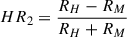 , where Ri is the count rate for energy band i.
The observed hardness ratios of HD 166620 are HR1 = −0.44 ± 0.13 and 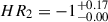 . Using XSPEC, we created a simulated APEC spectrum with the EPIC/pn instrumental response files of the observation for the dominating component from the spectral fit at a temperature of
  (see Sect. 2.2). For the simulated spectrum, we obtained the count rate for each of the aforementioned energy bands and we computed the “expected" hardness ratios for a star with that mean coronal temperature. The resulting values of HR1sim = −0.55 and HR2sim = −0.99 are consistent with the observed values, showing the validity of the spectral model.
Appendix C: Rate-to-flux conversion factors
Catalogued X-ray count rates in energy band i, CRi, can be converted into a flux in energy band j, fj, if the corresponding conversion factor (CFij) is known. The CFij is computed as
 (C.1)
(C.1)
The CF depends on the characteristics of the instrument and the spectral shape of the observed emission. In the X-ray catalogues used in this article, the source count rates have been corrected for PSF-loss and vignetting effects and are thus handled as on-axis count rates with an infinite extraction radius.
We simulate the typical X-ray spectrum of an FGK dwarf in XSPEC, using the best-fit model determined from an analysis of the average eRASS spectrum of all FGK dwarfs within 10 parsec (Zheng et al. 2025). This model is a three-temperature variable abundance (3T-VAPEC) model. Using the flux routine in XSPEC, we obtain the flux in the 0.1–2.4 keV ROSAT energy band from the model. Then we use the fakeit routine to convolve the simulated spectrum with the specific response matrix of each instrument to compute an expected count rate for the energy band used in the catalogue.
In the following, we briefly discuss considerations for each instrument used. All calculated CFs are presented in Table C.1.
Instrument-specific CFs to convert count rates for FGK dwarfs into 0.1–2.4 keV ROSAT band fluxes.
ROSAT
For 2RXS observations the instrument PSPC-C was used. We use the response file pspcc_gain1_256.rsp from HEASARC2, which already contains the on-axis effective area.
In our sample, all 2RXP observations use the PSPC-B detector. For observations before the destruction of the PSPC-C and the corresponding change in detector gain of PSPC-B on 1991-10-14, the appropriate file is pspcb_gain1_256.rsp. For later observations, we use pspcb_gain2_256.rsp.
eROSITA
As part of the first eROSITA data release (Merloni et al. 2024), the calibration products were made public. For the catalogue count rates, the appropriate files are provided as onaxis_tm0_rmf_2023-01-17.fits and onaxis_tm0_arf_filter_2023-01-17.fits.
XMM-Newton
In this article, we only consider count rates from EPIC/pn. ESA provides ‘canned’ response matrices3. Catalogue values are provided for “single + double” imaging patterns, and the appropriate file is epn_e4_ff20_sdY9_v22.0.rmf.
The on-axis ancillary files are generated with the arfgen command in SAS. To mitigate PSF-losses, we choose a large extraction region of 5 arcmin. The EPIC/pn observations of our sample were carried out using the “thick" or the “medium" filter. The different transmissions of the EPIC/pn filters are taken into account with individual ancillary files. For completeness, we provide the CF for the “thin" filter, too.
Cross-calibration
Stars in our sample that were observed by multiple instruments allow us to verify the CFs by comparing the X-ray luminosities derived from the different instruments, as presented in Fig. C.1. We notice a systematic trend where objects appear brighter in ROSAT observations compared to eROSITA or XMM-Newton.
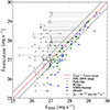 |
Fig. C.1. Comparison of X-ray luminosities detected with 2RXS, eROSITA, and XMM-Newton in the ROSAT energy band after applying the respective CF shown in Table C.1. For the M10pc sample, we use the CFs from Caramazza et al. (2023). Black bars represent the sensitivity limit of 2RXS at the individual distances of the stars. |
This trend is most significant for fainter objects (log LX, 2RXS (erg s−1) ≲ 27.5) where the difference can be explained by an observational bias due to the lower sensitivity of ROSAT, combined with intrinsic variability of the stars. Namely, X-ray faint stars (lower left of the diagram) were detectable in 2RXS only if they were brighter than during their observation with XMM-Newton or eRASS. This is illustrated in Fig. C.1 with black vertical dashes, which represent the individual approximate 2RXS X-ray luminosity limits, derived from the RASS flux limit of fX ≈ 10−13 erg cm−2 s−1 (Boller et al. 2016). For the faintest stars this limit is above their LX value measured with the more sensitive instruments, XMM-Newton or eROSITA. Similar observations were made on other samples by, e.g., Magaudda et al. (2022), Freund et al. (2018), Zhu & Preibisch (2025).
A systematic offset is also seen for the brighter regime (log LX, 2RXS (erg s−1) ≳ 27.5), albeit at a smaller scale. A possible origin for this trend might be calibration differences not fully captured in the instrument response files. Moreover, the spectral model of the average FGK dwarf (Zheng et al. 2025) used to compute the CFs was obtained from a fit to the eRASS spectrum in the 0.35–2.0 keV energy band and had to be extrapolated to cover the full ROSAT energy band which may lead to an underpredicted soft emission. The spectral 3T-VAPEC model of the average FGK dwarf has an emission-weighted mean temperature of  . For stars with cooler coronae, this could lead to an underestimated flux in the low energy range. In fact, the dominating spectral component of HD 166620 is at a temperature of
  and its effective conversion factor from the count rates of source detection to the flux in the ROSAT-band is
 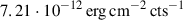 , which is a factor 4.2 higher than the CF determined for a “medium” filter XMM-Newton observation. While HD 166620 is an extreme example, it shows that for other FGK dwarfs with very soft X-ray emission, the CFs for XMM-Newton and eROSITA may be underestimated. In that case, the true X-ray luminosities of such stars observed by XMM-Newton and eROSITA would be higher, putting them closer to the values observed with ROSAT.
Appendix D: Isochrone fitting
We obtain fundamental stellar parameters for our sample from fitting isochrones on the colour-magnitude diagram. The isochrones are adopted from the PARSEC V2.0 database (Nguyen et al. 2022, 2025), without rotation. To perform the fit, we use Gaia colours where available, and Johnson B-V-colours otherwise. A grid of isochrones is created with ages spanning from 0.5 to 9.0 Gyr with a step-size of 0.5 Gyr, and metallicities ([M/H]) in the range from -1.5 to 0.5 dex with a step-size of 0.1 dex. We use metallicities from Soubiran et al. (2022) where available and else from Gáspár et al. (2016), Sousa et al. (2008) to constrain the isochrones, while leaving the age free to be fit. We assume that [Fe/H] ≈ [M/H] as the sample is limited to the nearby solar neighbourhood, which is part of the thin disk and thus not significantly alpha-enhanced (Bensby et al. 2014; Buder et al. 2019).
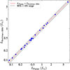 |
Fig. D.1. Bolometric luminosities for our sample obtained with PARSEC V2.0 compared with those published by Soubiran et al. (2024). The dashed lines mark a deviation of 10%. |
For an isochrone of matching metallicity, the best-fit value is determined by the minimum distance between the observed data and the points of the isochrone in the colour-magnitude-space. In case there is no exact match with the observed metallicity due to the limited resolution of the grid, we linearly interpolate between the best-fit values of the two closest metallicities. As a result, we obtain fundamental parameters such as the bolometric luminosity and effective temperature of the star.
From the FGK 10pc sample, 25 dwarfs are also part of the Gaia FGK benchmark stars (Soubiran et al. 2024). A comparison of our values for the bolometric luminosity with the values from Soubiran et al. (2024) shows an agreement well within 10%, as depicted in Fig. D.1.
All Tables
Instrument-specific CFs to convert count rates for FGK dwarfs into 0.1–2.4 keV ROSAT band fluxes.
All Figures
|
Fig. 1. SHK and RX time series for HD 166620 with data compiled by Luhn et al. (2022) and more recent data from Keck/HIRES (Isaacson et al. 2024) and the APF (Vogt et al. 2014). The small transparent symbols mark individual SHK measurements, and the larger opaque symbols are the same data, binned in 120 d bins. A black outline denotes a bin containing only a single measurement. The dashed blue line shows the extrapolated trend of the two maxima (see Sect. 2.1). The two X-ray measurements are overplotted with black squares, and their epochs are marked on the axis. |
| In the text | |
|
Fig. 2. Top: XMM-Newton EPIC/pn spectrum of HD 166620 and best-fit 2T-APEC thermal model. Bottom: Residuals. |
| In the text | |
|
Fig. 3. X-ray over bolometric luminosity for HD 166620 in its two detections compared with the range of values observed throughout the solar cycle (Peres et al. 2000) and for FGK (Bennedik et al., in prep.) and M0–M4 dwarfs (Caramazza et al. 2023) within 10 pc of the Sun. |
| In the text | |
|
Fig. 4. Same as Fig. 3, but for X-ray surface fluxes FX. The typical ranges of FX exhibited by different types of solar coronal structures (from Caramazza et al. 2023) are depicted as coloured stripes. |
| In the text | |
|
Fig. A.1. SHK time series for HD 166620 showing the Keck/HIRES data in comparison with the newly obtained APF data. The dotted vertical line marks the time of the XMM-Newton observation. |
| In the text | |
|
Fig. C.1. Comparison of X-ray luminosities detected with 2RXS, eROSITA, and XMM-Newton in the ROSAT energy band after applying the respective CF shown in Table C.1. For the M10pc sample, we use the CFs from Caramazza et al. (2023). Black bars represent the sensitivity limit of 2RXS at the individual distances of the stars. |
| In the text | |
|
Fig. D.1. Bolometric luminosities for our sample obtained with PARSEC V2.0 compared with those published by Soubiran et al. (2024). The dashed lines mark a deviation of 10%. |
| In the text | |
Current usage metrics show cumulative count of Article Views (full-text article views including HTML views, PDF and ePub downloads, according to the available data) and Abstracts Views on Vision4Press platform.
Data correspond to usage on the plateform after 2015. The current usage metrics is available 48-96 hours after online publication and is updated daily on week days.
Initial download of the metrics may take a while.