© The Authors 2026

1. Introduction

The assembly, abundance and clustering of dark matter haloes play an important role both in galaxy formation and in the ongoing efforts to constrain cosmological parameters, where it is crucial to model accurately how haloes and galaxies trace the matter density field. While the latter is continuous, though, at least above some scale, the halo centres of mass define a point process at a given time, and the same is true at the initial time for the centres of mass of the protohalo patches from which they formed Bardeen et al. (1986). Therefore, models of halo collapse and formation seek to identify what makes these locations special in the initial fluctuation field. Such studies make two types of choices: what the ‘field’ is, and what the ‘properties’ of this field are.

Following Gunn & Gott (1972), who described halo formation as the collapse of a homogeneous sphere, most of the literature on the subject has assumed that the initial matter overdensity field is the one of interest. However, haloes are not spherical. Thus, some early works suggested that the ‘shape tensor’ – identified with the Hessian of the matter density field, that is, the 3 × 3 matrix of the second spatial gradients – provides useful additional information about departures from sphericity (Bardeen et al. 1986; van de Weygaert & Bertschinger 1996).

Other authors focused on a different 3 × 3 matrix: the ‘deformation tensor’ – constructed from the volume average of the second gradients of the gravitational potential – noting that it is dynamically more interesting (Doroshkevich 1970; Bond & Myers 1996). Indeed, in the homogeneous ellipsoidal collapse model studied by Bond & Myers (1996), an initially spherical region is deformed by the surrounding shear field: hence the name ‘deformation’ tensor (routinely used in fluid dynamics, although usually referring to infinitesimal volumes, not to the average over macroscopic regions). The mean matter overdensity, thanks to Poisson’s equation, is the trace of the deformation tensor; and since the trace is the sum of the three eigenvalues, this raises the question whether the 3 eigenvalues (or their linear combinations) themselves play an important role, or if only their sum matters.

Any 3 × 3 matrix also has three ‘rotational invariants’. These are the coefficients of its characteristic polynomial, whose roots are the eigenvalues, and provide an alternative description of the same information. Since the trace is just one of the three, it is natural to ask what role the other two, which are non-linear combinations of the eigenvalues, play. This is particularly interesting in view of the fact that rotational invariants have been used to quantify how protohaloes correlate with their environment (Desjacques 2013; Lazeyras et al. 2016; Lazeyras & Schmidt 2018).

Indeed, the second order invariant of the deformation tensor – the amplitude of the traceless shear – matters for halo formation: protohaloes with larger shear tend to be more overdense (Sheth et al. 2001; Despali et al. 2013), and this sources a correlation with the environment on larger scales (Sheth et al. 2013; Modi et al. 2017; Lazeyras & Schmidt 2018). This is slightly surprising because, in a Gaussian random field, the two invariants are statistically independent (Sheth & Tormen 2002). Therefore, we want to investigate what aspect of halo formation induces the measured correlation between overdensity and shear, since this another manifestation of what makes protohalo positions special.

Recently, it has been highlighted that, as a ‘field’, the initial energy overdensity is more interesting than the initial matter overdensity (Musso & Sheth 2021). Indeed, the energy shear tensor is more directly related to the physics of collapse than is the deformation tensor (Musso et al. 2024). This implies that, unlike the deformation tensor, the energy shear is almost always positive definite. Moreover, just as for the deformation tensor and even more strongly, the first and second invariants of the energy shear are positively correlated.

With this in mind, our study has two main goals. First, does the third invariant (of the energy shear tensor) also matter? And second, can the correlations between the invariants of the protohalo patches be understood as simply arising from the positivity constraint?

In the next section, we define the three invariants, before showing that all three play an important role in characterising the properties of protohalo patches. Then we show that requiring positivity induces correlations between the invariants, which are qualitatively similar to those exhibited by protohaloes. While positivity implies that an object will collapse, it does not determine when the collapse is complete: Section 3 discusses how collapse by a specified time can be associated with a threshold in the energy overdensity. It then explores if this threshold depends on other invariants (than the trace) as well. A final section summarises our conclusions.

2. Rotational invariants of protohaloes

The energy overdensity tensor of a generic comoving volume V, or energy shear, is the 3 × 3 matrix

$$\begin{array}{c}\hfill u_{\mathit{ij}}\equiv \frac{3}{I}{\displaystyle {\int }_V}\mathrm{d}\mathit{r}\rho (\mathit{r},t)(r_i-r_{\mathrm{cm},i})({\mathrm{\nabla }}_j\varphi -{[{\mathrm{\nabla }}_j\varphi ]}_{\mathrm{cm}})\end{array}$$(1)

as defined by Musso et al. (2024), where ρ is the matter density, ϕ is the potential energy perturbation (related to the matter density contrast $\delta =\rho /\overline{\rho }-1$ by the Poisson equation ∇²ϕ = δ), r_cm ≡ (1/M)∫_Vdrρ(r, t)r and [∇ϕ]_cm ≡ (1/M)∫_Vdrρ(r, t)∇ϕ are the centre of mass position and acceleration, and I ≡ ∫_Vdrρ(r, t)|r − r_cm|² is the moment of inertia.

At very early times, when ρ is nearly uniform and ϕ is a nearly Gaussian field, measuring u_ij at generic positions returns a Gaussian random matrix. If V is a randomly placed sphere of radius R, and only in this case, the covariance of the energy shear can be expressed as

$$\begin{array}{c}\hfill \langle u_{\mathit{ij}}{u}_{\mathit{kl}}\rangle =\frac{{\delta }_{\mathit{ik}}{\delta }_{\mathit{jl}}+{\delta }_{\mathit{il}}{\delta }_{\mathit{jk}}+{\delta }_{\mathit{ij}}{\delta }_{\mathit{kl}}}{15}{\sigma }_{02}^2,\end{array}$$(2)

where the Gaussian moment

$$\begin{array}{c}\hfill {\sigma }_{02}^2(R)\equiv {\displaystyle \int \frac{\mathrm{d}\mathit{k}}{{(2\pi )}^3}}\delta (\mathit{k})\frac{15j_2(kR)}{{(kR)}^2}\end{array}$$(3)

is the variance of the trace of u_ij, or energy overdensity (Musso & Sheth 2021). All higher cumulants of the distribution vanish. Since $M=(4\pi /3)\overline{\rho }{R}^3$, σ₀₂ encodes the mass dependence of the distribution.

However, as pointed out recently by Musso et al. (2024), u_ij also sources the evolution of the inertia tensor I_ij of the body. Therefore, if V is a protohalo, the energy shear (more precisely, its symmetric part u_ij + u_ji) must have three positive eigenvalues for the volume to collapse along three axes. In other words, measuring u_ij in protohaloes no longer yields a Gaussian random matrix, but a positive definite one.

2.1. Rotational invariants of positive definite matrices

Regardless of its signature, the symmetric part u_ij + u_ji of the energy shear has three real eigenvalues λ₁ > λ₂ > λ₃, a priori not necessarily positive, in terms of which one can construct the three rotational invariants

$$\begin{array}{cc}& ϵ\equiv {\displaystyle \sum _i}{\lambda }_i,q^2\equiv \frac{3}{2}{\displaystyle \sum _i}{({\lambda }_i-ϵ/3)}^2,\mathrm{and}\hfill \\ \hfill & U^3\equiv {\displaystyle \sum _i}{({\lambda }_i-ϵ/3)}^3=3{\displaystyle \prod _i}({\lambda }_i-ϵ/3).\hfill \end{array}$$(4)

The trace ϵ = tr(u) is the energy overdensity; in terms of ${\overline{u}}_{\mathit{ij}}\equiv u_{\mathit{ij}}-ϵ{\delta }_{\mathit{ij}}/3$, the traceless part of the matrix, $q^2=3\mathrm{tr}({\overline{\mathbf{u}}}^2)/2$ is the traceless shear amplitude; and $U^3=\mathrm{tr}({\overline{\mathbf{u}}}^3)=3det({\overline{\mathbf{u}}}^3)$ is (thrice) the traceless determinant.

The equation for the eigenvalues can be conveniently written in the form of a depressed cubic as

$$\begin{array}{c}\hfill {[(3\lambda -ϵ)/q]}^3-3[(3\lambda -ϵ)/q]-2\mu =0,\end{array}$$(5)

where

$$\begin{array}{c}\hfill \mu \equiv (9/2)(U^3/q^3);\end{array}$$(6)

for this equation to admit three real solutions, as it should be since the matrix is symmetric, the constraint μ² < 1 must be satisfied, or equivalently −1 ≤ μ ≤ 1. Clearly, one also has $q\equiv \sqrt{q^2}\ge 0$. The roots of the cubic equation are then

$$\begin{array}{c}\hfill {\lambda }_k=\frac{ϵ}{3}+\frac{2q}{3}cos[\frac{1}{3}arccos(\mu )-\frac{2\pi }{3}(k-1)],\end{array}$$(7)

which expresses the three eigenvalues in terms of the three rotational invariants. Configurations with μ ≃ 1 have λ₁ > λ₂ ≃ λ₃, whereas μ ≃ −1 implies λ₁ ≃ λ₂ > λ₃, and μ ≃ 0 implies λ₂ ≃ ϵ/3. Figure 1 shows the three eigenvalues as a function of μ. Evidently, 3(λ₁ − λ₃)/q ≈ 3 for all values of μ, meaning that λ₁ − λ₃ ≈ q. Hence, the ellipticity e_u ≡ (λ₁ − λ₃)/2ϵ ≈ q/2ϵ.

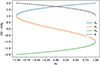Fig. 1. Ratio of traceless eigenvalues to q/3 as a function of μ (equation 7). Also shown (dashed line) is the function X(μ) defined in equation (10), marking the lower limit of ϵ/q.

Regardless of the sign of the eigenvalues, the rotational invariants always satisfy the relations

$$\begin{array}{cc}& {ϵ}^2-q^2=3({\lambda }_1{\lambda }_2+{\lambda }_1{\lambda }_3+{\lambda }_2{\lambda }_3)\mathrm{and}\hfill \end{array}$$(8)

$$\begin{array}{cc}& 2\mu +\frac{ϵ}{q}(\frac{{ϵ}^2}{q^2}-3)=27\frac{det(\mathbf{u})}{q^3}=27\frac{{\lambda }_1{\lambda }_2{\lambda }_3}{q^3}·\hfill \end{array}$$(9)

If however u_ij is positive definite (that is, if all its eigenvalues are positive), the right-hand sides of equations (8) and (9) are both positive; so ϵ > q and (ϵ/q)³ − 3(ϵ/q)+2μ > 0. The equation associated with the latter inequality is the same as the equation for (ϵ − 3λ)/q, and its roots can be obtained from equation (7).

The only root larger than 1 (required since ϵ > q) is the one obtained by plugging in λ₃. Therefore, all eigenvalues are positive if (and only if)

$$\begin{array}{c}\hfill \frac{ϵ}{q}>-2cos[\frac{arccos(\mu )-4\pi }{3}]\equiv X(\mu )\end{array}$$(10)

(which also implies that ϵ > q). Clearly, this is the same as requesting that λ₃ > 0, since X(μ) is equal to (ϵ − 3λ₃)/q. Using trigonometric identities, X(μ) can also be expressed as

$$\begin{array}{c}\hfill X(\mu )=2cos[\frac{arccos(-\mu )}{3}],\mathrm{with}1\le X\le 2.\end{array}$$(11)

Its numerical value is also shown in Fig. 1 (dashed line).

Although we have focused on rotational invariants, other combinations of eigenvalues were featured in previous work (Bardeen et al. 1986; Bond & Myers 1996; Sandvik et al. 2007). Quantities built from linear combinations of the eigenvalues tend to all have the same structure: one variable is the trace, which we denote ϵ, and the two other ones are formed from differences with respect to one of the eigenvalues (i.e. they are constructed from the traceless matrix). For example,

$$\begin{array}{c}\hfill v_{\pm }=({\lambda }_1-{\lambda }_3)\pm ({\lambda }_2-{\lambda }_3),\end{array}$$(12)

which obviously has v_± ≥ 0 and 0 ≤ v₋ ≤ v₊. The shape parameters y and z defined in equation (A.2) of Bardeen et al. (1986) are formed from the differences of the other eigenvalues with respect to λ₂ rather than λ₃. (The ellipticity and prolateness of Bond & Myers 1996 are conceptually the same: differences with respect to the middle eigenvalue). Our v_± variables were considered by Sandvik et al. (2007), although they had no real physical justification for their choice. Likewise, one could have worked with differences with respect to λ₁. We prefer differences with respect to λ₃ because the positivity constraint (λ₃ ≥ 0) is particularly simple in these variables. This is because

$$\begin{array}{c}\hfill v_{+}={\lambda }_1+{\lambda }_2-2{\lambda }_3=ϵ-3{\lambda }_3=qX(\mu );\end{array}$$(13)

so, positivity requires ϵ ≥ 0 and 0 ≤ v₊ ≤ ϵ, but the v₋ range is unchanged (0 ≤ v₋ ≤ v₊). As we show below, this makes it easy to describe the joint distribution of (ϵ, v₊, v₋) when all three eigenvalues are positive.

2.2. Protohalo properties

We studied the properties of the protohaloes of haloes identified at z = 0 using a spherical overdensity halo finder with a threshold of 319 times the background density, in the Bice and Flora simulations of the SBARBINE suite (Despali et al. 2016). For both simulations, the background cosmology has Ω_m = 0.307, Ω_Λ = 0.693, σ₈ = 0.829 and h = 0.677. Each one contains 1024³ dark matter particles in a periodic box of side L_box = 125 h⁻¹ Mpc (Bice) and L_box = 2 h⁻¹ Gpc (Flora); hence, the corresponding particle masses are 1.55 × 10⁸ h⁻¹ M_⊙ for Bice and 6.35 × 10¹¹ h⁻¹ M_⊙ for Flora.

Our Bice sample contains 5000 randomly selected haloes with masses between 10¹¹ and 4 × 10¹³ h⁻¹ M_⊙. Our Flora sample contains haloes from three separate mass bins, as follows: 2000 randomly selected haloes with masses between 4 × 10¹³ and 10¹⁴ h⁻¹ M_⊙, 2000 randomly selected haloes with masses between 10¹⁴ and 10¹⁵ h⁻¹ M_⊙, and all 1378 haloes more massive than 10¹⁵ h⁻¹ M_⊙. In the following, we will indicate these three samples as Flora-S, Flora-M and Flora-L respectively.

For each halo identified at z = 0, we refer to the region occupied by the halo particles in the initial conditions as ‘protohalo’. Following Musso et al. (2024), we measured each protohalo’s centre of mass position and velocity, q_cm and v_cm, by averaging over all its particles. We then estimated its energy shear tensor as

$$\begin{array}{cc}\hfill {\widehat{u}}_{\mathit{ij}}& \equiv -3\frac{{\sum }_{n=1}^{N_H}{({\mathit{q}}^{(n)}-{\mathit{q}}_{\mathrm{cm}})}_i{({\mathit{v}}^{(n)}-{\mathit{v}}_{\mathrm{cm}})}_j/fDH}{{\sum }_{n=1}^{N_H}{|{\mathit{q}}^{(n)}-{\mathit{q}}_{\mathrm{cm}}|}^2},\hfill \end{array}$$(14)

where D is the ΛCDM density perturbation growth factor (at the redshift z of the snapshot), f = dlnD/dlna, and n runs over the N_H protohalo particles. (Note that u_ij is a ‘dimensionless energy’ because at early times the velocity is proportional to the acceleration, which is the gradient of the gravitational potential: $\mathrm{\nabla }\varphi \simeq \mathit{v}/\dot{D}=\mathit{v}/fDH$). We then diagonalise ${\widehat{u}}_{\mathit{ij}}$ and estimate ϵ, q and μ using Eq. (4).

Figure 2 (top panel) shows a scatter plot of ϵ vs q. The colour indicates the value of μ, measured in the same set of protohaloes of Musso et al. (2024), where the underlying cosmology and halo identification schemes are described. Indeed, the points here are the same as in their Figure 10; the only difference is that we have coloured each point by its (protohalo’s) value of μ. Clearly, the three invariants are strongly correlated, with higher shear values corresponding to higher ϵ. Moreover, the slope of this nearly linear scaling depends on the third invariant: points with larger μ (coloured in yellow) have shallower ϵ − q slopes, and tend to be lower and to the right compared to points with smaller μ (violet). The latter are confined to the left part of the plot. The dashed lines show the theoretical lower limit for different values of μ: their slopes are {1, 4/3, 5/3, 2} from bottom to top, corresponding to μ = {1, 0.815, 0.185, −1}.

Before we discuss the dashed lines further, we note that the distribution in the top panel is remarkable because, for generic Gaussian matrices, and thus for tensors measured at generic positions in a Gaussian random field, any variables constructed from the traceless part of the matrix should be uncorrelated with the trace. Therefore, their trace would be a Gaussian variate with zero mean, and their shear an independent χ₅ variate (see discussion following equation 19). The third rotational invariant μ, constructed from the determinant, should also be independent, with a flat distribution between −1 and 1. Since the distribution in the top panel of Figure 2 clearly has ϵ ≥ 2, it is completely different from that for random positions in a Gaussian field.

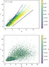Fig. 2. Top panel: Correlation between the three rotational invariants of protohaloes: energy overdensity ϵ, the traceless energy shear q, and μ (see equation 4). The colour displays the value of μ. The dashed lines show ϵ = nq for n = {1, 4/3, 5/3, 2} (from bottom to top), corresponding to the minimum value of ϵ for μ = {1, 0.815, 0.185, −1} whenever the energy shear tensor is positive definite – as shown by equation (10). Bottom panel: Expected distribution of ϵ − q and μ if protohaloes where centred on random locations constrained to have the measured values of ϵ (typically ϵ ≳ 2).

To test if the distribution of the trace is different, but the distributions of q and μ are not otherwise special, the bottom panel of Figure 2 shows how the same ϵ − q plot would look if q and μ were independent variables. To generate this plot, we used the measured values of ϵ and σ₀₂, but replaced q and μ with two random variables drawn, respectively, from a χ distribution with 5 degrees of freedom (with the same values of σ₀₂) and a distribution that is uniform between −1 and 1. This bottom panel is very different from the top one: evidently, the distributions of q and μ are also special.

The correlation shown in the upper panel of Fig. 2 provides some insight into the reason for this behaviour. As a precursor of one of our results, we consider what happens if the energy shear is positive definite, as Musso et al. (2024) showed it must be for protohalo patches. Then, as discussed in Section 2.1, it must be that ϵ > q. This introduces the linear correlation seen in Fig. 2. Secondly, equation (10) must be satisfied, and, since its r.h.s. is a decreasing function of μ, protohaloes with μ closer to −1 are constrained to have larger ϵ/q. This explains why, as one moves away from the lower dashed line in the top panel of Fig. 2 (indicating where ϵ = q), the value of μ tends to decrease. The three steeper dashed lines indicate the lower limit for haloes with ϵ/q larger than 4/3, 5/3 and 2 respectively (corresponding to μ of .185, .815 and 1). Moreover, as shown by equation (8), for a positive definite matrix the inequality ϵ > q is saturated only if all three eigenvalues simultaneously vanish, which never happens in practice.

Figure 3 (top panel) shows the values of ϵ versus the third rotational invariant μ, coloured by the logarithm of the mass. The yellow and green bands at the bottom correspond to the Flora-L, Flora-M and Flora-S samples, and are quite uniformly distributed between −1 and 1. Conversely, Bice haloes (lower mass) correspond to the violet dots of the upper band, and show a clear tendency to prefer values closer to 1. This behaviour can also be understood from equation (10), since for equal values of q protohaloes with μ ≃ −1 must have twice as large values of ϵ as those with μ ≃ 1, and are therefore less likely. Furthermore, except for a few low-mass outliers, in all protohaloes ϵ is larger than roughly 2.2 (we will denote this bottom value ϵ_c in the following), and tends to be higher at smaller masses. The trend of ϵ with mass and q are mutually compatible, since high-mass haloes prefer small values of q and thefore lie in the bottom left corner of Fig. 2.

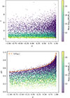Fig. 3. Correlation of ϵ (top panel) and q/ϵ (bottom) with μ for protohaloes, coloured by log10(M/h−1 M⊙). The dashed line in the bottom panel shows the upper limit given by (the inverse of) equation (10).

The bottom panel of Fig. 3 shows the value of the ratio q/ϵ: the upper cut determined by (the inverse of) equation (10) (dashed line in the plot) is clearly visible. This bound affects the low-mass Bice haloes the most. High-mass protohaloes have small q, but nevertheless have (as the top panel shows) non-zero ϵ. Therefore, their q/ϵ is naturally low, and mostly unaffected by the presence of an upper bound.

The fact that the correlation pattern is explained by the ϵ > qX(μ) constraint motivates us to look at the correlation structure with the variables v₊ = qX and v₋ defined in equation (12). As shown in Figure 4, the linear correlation between ϵ and v₊ is even more prominent, with a scatter that becomes significantly narrower at high values. Points in the graph are coloured by the value of v₋/v₊ in each protohalo: the fact that colours are uniformly distributed in the plot shows that there is no residual correlation of ϵ − v₊ with v₋/v₊.

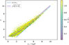Fig. 4. Correlation of ϵ with v+, with colours showing the value of v−/v+. The scatter is significantly narrower than in Figure 2, especially at higher values, and there is no residual correlation signal with v−/v+. Dashed line shows the theoretical lower limit ϵ = v+, and solid line shows $\sqrt{{ϵ}_c^2+v_{+}^2}$ with ϵc = 2.2.

2.3. Distribution of rotational invariants of positive-definite matrices

To simplify notation, in this section and in the following ones we set σ₀₂ = 1, unless otherwise specified. The distributions of ϵ and q presented here should therefore be read as those of ϵ/σ₀₂ and q/σ₀₂. Since it is defined as a ratio of variables, μ is not affected by this choice.

Doroshkevich (1970) showed that the joint distribution of the three eigenvalues of a 3 × 3 symmetric Gaussian matrix is given by

$$\begin{array}{c}\hfill p({\lambda }_1,{\lambda }_2,{\lambda }_3)=\frac{3^3{5}^3}{8\pi \sqrt{5}}{\mathrm{e}}^{-{ϵ}^2/2}{\mathrm{e}}^{-5q^2/2}\mathrm{\Delta }({\lambda }_1,{\lambda }_2,{\lambda }_3),\end{array}$$(15)

where ϵ and q² were defined earlier and

$$\begin{array}{c}\hfill \mathrm{\Delta }\equiv ({\lambda }_1-{\lambda }_2)({\lambda }_1-{\lambda }_3)({\lambda }_2-{\lambda }_3)\end{array}$$(16)

is the Vandermonde determinant. In terms of the rotational invariants ϵ, q and μ this distribution is

$$\begin{array}{c}\hfill p({\lambda }_1,{\lambda }_2,{\lambda }_3)\mathrm{d}{\lambda }_1\mathrm{d}{\lambda }_2\mathrm{d}{\lambda }_3=\mathcal{N}(ϵ)\chi (q)\frac{\mathrm{\Theta }(1-{\mu }^2)}{2}\mathrm{d}ϵ\mathrm{d}q\mathrm{d}\mu ,\end{array}$$(17)

where

$$\begin{array}{c}\hfill \mathcal{N}(ϵ)\mathrm{d}ϵ=\frac{{\mathrm{e}}^{-{ϵ}^2/2}}{\sqrt{2\pi }}\mathrm{d}ϵ\end{array}$$(18)

and

$$\begin{array}{c}\hfill \chi (q)dq=\frac{d{q}^2}{q^2}{\left(\frac{5q^2}{2}\right)}^{5/2}\frac{{\mathrm{e}}^{-5q^2/2}}{\mathrm{\Gamma }(5/2)}·\end{array}$$(19)

Therefore, ϵ is Gaussian distributed, 5q² follows a chi-square distribution with five degrees of freedom, and μ is uniform over [ − 1, 1]. In particular, we note that the distributions of ϵ, q and μ are independent; hence, the joint distribution above cannot explain the correlations seen in Figure 2.

This changes when all three eigenvalues have the same sign. If we require λ₃ > 0, then q < ϵ and 2μ > (ϵ/q)(3 − ϵ²/q²). In turn, this requires that max[−1, (ϵ/2q)(3 − ϵ²/q²)] < μ < 1. So, integrating over μ returns 1 if q < ϵ/2, but [(ϵ/2q)(ϵ²/q² − 3)+1]/2 if ϵ/2 < q < ϵ. The latter factors as (ϵ/q + 2)(ϵ/q − 1)²/2. Hence, the probability of having all positive eigenvalues is

$$\begin{array}{cc}\hfill p(+)& \equiv p({\lambda }_3\ge 0)\hfill \\ \hfill & ={\displaystyle {\int }_0^{\infty }}\mathrm{d}ϵ\mathcal{N}(ϵ)[{\displaystyle {\int }_0^{ϵ/2}}\mathrm{d}q\chi (q)\hfill \\ \hfill & +{\displaystyle {\int }_{ϵ/2}^{ϵ}}\mathrm{d}q\chi (q)\frac{(ϵ/q+2){(ϵ/q-1)}^2}{2}]\hfill \\ \hfill & =\frac{1}{2}-\frac{3arctan(\sqrt{5})+2\sqrt{5}}{6\pi }\approx \frac{2}{25}·\hfill \end{array}$$(20)

With this normalisation, the conditional distributions are

$$\begin{array}{cc}\hfill p(ϵ|+)& =\frac{\mathcal{N}(ϵ)}{p(+)}[{\displaystyle {\int }_0^{ϵ/2}}\mathrm{d}q\chi (q)\hfill \\ \hfill & +{\displaystyle {\int }_{ϵ/2}^{ϵ}}\mathrm{d}q\chi (q)\frac{(ϵ/q+2){(ϵ/q-1)}^2}{2}]\hfill \\ \hfill & =\frac{\mathcal{N}(ϵ)}{2p(+)}[\mathrm{erf}\left(\frac{ϵ}{2}\sqrt{\frac{5}{2}}\right)+\mathrm{erf}\left(ϵ\sqrt{\frac{5}{2}}\right)\hfill \\ \hfill & -3\sqrt{5}ϵ\frac{{\mathrm{e}}^{-5{ϵ}^2/8}}{\sqrt{2\pi }}],\hfill \end{array}$$(21)

$$\begin{array}{cc}\hfill p(q|+)& =\frac{\chi (q)}{p(+)}[{\displaystyle {\int }_{2q}^{\infty }}\mathrm{d}ϵ\mathcal{N}(ϵ)\hfill \\ \hfill & +{\displaystyle {\int }_q^{2q}}\mathrm{d}ϵ\mathcal{N}(ϵ)\frac{(ϵ/q+2){(ϵ/q-1)}^2}{2}]\hfill \\ \hfill & =\frac{\chi (q)}{4p(+)}[\mathrm{erfc}(q/\sqrt{2})+\mathrm{erfc}(q\sqrt{2})\hfill \\ \hfill & -\frac{{\mathrm{e}}^{-2q^2}(q^2+2)+2{\mathrm{e}}^{-q^2/2}(q^2-1)}{q^3\sqrt{2\pi }}],\hfill \end{array}$$(22)

$$\begin{array}{cc}\hfill p(\mu |+)& =\frac{1}{2p(+)}{\displaystyle {\int }_0^{\infty }}\mathrm{d}q\chi (q){\displaystyle {\int }_{X(\mu )q}^{\infty }\mathrm{d}ϵ\mathcal{N}}(ϵ)\hfill \\ \hfill & =\frac{1}{2\pi p(+)}[\mathrm{arccot}\left(\frac{X}{\sqrt{5}}\right)-\frac{\sqrt{5}X(3X^2+25)}{3{(X^2+5)}^2}],\hfill \end{array}$$(23)

where X(μ) was defined in equation (11).

This shows that requiring positive definiteness shifts the distribution of ϵ so that high values are more likely (e.g. its mean is non-zero, close to 1.65); it shifts the distribution of q so that high values are less likely; it induces a correlation between ϵ and q; and it changes the distribution of μ so that values of unity are more likely. For instance, some of the relevant moments are:

$$\begin{array}{cc}& ⟨ϵ|+⟩\simeq 1.665\approx 5/3,⟨{ϵ}^2|+⟩\simeq 3.067,\hfill \\ \hfill & ⟨u|+⟩\simeq 0.725\approx 29/40,⟨u^2|+⟩\simeq 0.587.\hfill \end{array}$$

The cross-correlation between ϵ and q is C_ϵu = ⟨ϵu|+⟩≃0.068. The expected slope of the ϵ − q relation is then C_ϵu/Var(u|+)≃0.068/0.063 ≈ 1, in agreement with Figure 4.

These distributions of ϵ, q and μ are shown by the dashed lines in Figs. 5 and 6 (the dotted lines correspond to the standard results for Gaussian matrices with unconstrained eigenvalues: normal, chi-5 and uniform). In each figure, the histograms correspond to the measurement of the same quantity in four halo samples (three filled histograms show Flora haloes; open histogram shows the less massive Bice sample). Figure 5 shows that, for high masses (filled histograms), the distribution of ϵ/σ₀₂ is strongly mass dependent and is not well described by equation (21). However, for low masses (leftmost histogram) the measurement tends to the predicted (mass-independent) result. This trend can be attributed to the fact that massive protohaloes have ϵ ≳ 2 but q ∼ σ₀₂ ≪ 2; so, they are almost insensitive to the positivity constraint ϵ > q. However, most lower-mass protohaloes have q > 2; so, for them ϵ > q is the dominant constraint, and this constraint explains most of their behaviour.

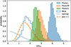Fig. 5. Distribution of trace ϵ/σ02 for a few ranges in halo mass (histograms). The dotted curve shows the expected (zero-mean, unit variance Gaussian) distribution at unconstrained positions; the dashed curve, at positions with λ3 ≥ 0 (Eq. 21). More massive haloes have larger ϵ/σ02, but the distribution around the mean is approximately independent of mass.

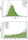Fig. 6. Distribution of traceless shear q/σ02 (top) and μ (bottom). The dotted curves show the expected distributions at unconstrained positions; the dashed ones, at positions with λ3 ≥ 0 (equations 22 and 23). Whereas q/σ02 is approximately the same for all masses, μ is closer to uniform as mass increases.

The top panel of Figure 6 displays the distribution of the traceless shear amplitude q/σ₀₂. In contrast to ϵ/σ₀₂, this shear shows remarkably little mass dependence: the four histograms lie almost on top of each other. Nevertheless, the measured values tend to be higher than predicted by p(q|+) (equation 22), shown by the dashed curve. The bottom panel shows the distribution of μ. In this case, values of μ closer to 1 become more likely, and the trend is more pronounced for less massive haloes. This is a consequence of the constraint X(μ) < ϵ/q: since small haloes have ϵ/q ∼ 1, values of μ closer to 1 are favoured, for which X(μ) is smaller (see bottom panel of Fig. 3). On the other hand, large haloes typically have ϵ/q ≫ 1, which makes the constraint less relevant (since 1 < X(μ) < 2). The same can also be inferred from Fig. 2: more and more haloes are excluded as the dashed line becomes steeper, but this does not affect the bottom left corner (where most massive haloes lie).

2.4. Linear combinations of eigenvalues

Figure 4 shows that the ϵ − v₊ relation has smaller scatter than ϵ − q. This motivated a study of the joint distribution of (ϵ, v₊, v₋), and of how it is affected by the positivity constraint.

Since v_± are formed from differences of eigenvalues, we expect them to be independent of the trace. Indeed, their joint distribution is (always with the σ₀₂ = 1 convention)

$$\begin{array}{c}\hfill p(ϵ,v_{+},v_{-})=\frac{{15}^3}{2^5}\frac{{\mathrm{e}}^{-{ϵ}^2/2}}{\sqrt{2\pi }}\frac{{\mathrm{e}}^{-5v_{+}^2/8-15v_{-}^2/8}}{\sqrt{90\pi }}{v}_{-}(v_{+}^2-v_{-}^2),\end{array}$$(24)

where an unconstrained Gaussian random field has −∞≤ϵ ≤ ∞, v₊ ≥ 0 and 0 ≤ v₋ ≤ v₊. Integrating over v₋ yields

$$\begin{array}{c}\hfill p(ϵ,v_{+})=\mathcal{N}(ϵ)\frac{{\mathrm{e}}^{-5v_{+}^2/8}}{\sqrt{2\pi /5}}({\mathrm{e}}^{-15v_{+}^2/8}-1+15v_{+}^2/8).\end{array}$$(25)

It is straightforward to check that integrating v₊ over the full range (v₊ ≥ 0) yields 𝒩(ϵ); and that, recalling that the positivity constraint is simply 0 ≤ v₊ ≤ ϵ (with the v₋ range unchanged), integrating over this restricted range returns p(ϵ|+) p(+). The distribution of v₊ subject to the constraint that λ₃ ≥ 0 is given by

$$\begin{array}{cc}\hfill p(v_{+}|+)& ={\displaystyle {\int }_{v_{+}}^{\infty }}dϵ\frac{p(ϵ,v_{+})}{p(+)}\hfill \\ \hfill & =\frac{{\mathrm{e}}^{-5v_{+}^2/8}}{\sqrt{2\pi /5}}({\mathrm{e}}^{-15v_{+}^2/8}-1+15v_{+}^2/8)\frac{\mathrm{erfc}(v_{+}/\sqrt{2})}{2p(+)}·\hfill \end{array}$$(26)

The final error function modifies the shape, effectively reducing the probability of large v₊.

3. From collapsing to collapsed

The positive-definite constraint is sensible from a dynamical point of view: bound objects should collapse along all three axes. However, Fig. 2 shows a clear lower limit, ϵ ≳ 2, that (for small q) is more stringent than the ϵ > q limit required by positive definiteness (lowest dashed line). This strongly suggests that something in addition to positive definiteness is required to explain the properties of protohaloes (in this case, the patches destined to be haloes by the present time, z = 0). Simply requiring λ₃ ≥ 0 does not constrain when the collapse is completed. There may be many objects that are collapsing now but have not yet collapsed completely, and others that collapsed earlier. This raises the question of what sets the time of collapse.

As shown by Musso & Sheth (2021), ϵ controls the evolution of the inertial radius of the halo; for a centrally peaked density profile, ϵ is always larger than mean enclosed matter overdensity, which controls the evolution of the geometric radius (related to the cubic root of the volume). In a simple spherical collapse model, the latter must have an initial overdensity of ∼1.7 for the required density to be assembled today (Gunn & Gott 1972). Since the final inertial radius is always smaller than the geometric radius, the threshold on ϵ must be even larger. Musso & Sheth (2021) showed that in large haloes, whose collapse should be fairly anisotropic, ϵ must equal a critical value: ϵ_c ≈ 2.

A simple calculation of the distribution of the three rotational invariants ϵ, q and μ subject to the additional constraint that ϵ > ϵ_c is given in Appendix A.1. However, the conditional pdf for ϵ resulting from this approach is simply the ϵ > ϵ_c tail of equation (21), appropriately normalized. None of our measurements is close to such a sharply cut distribution, and we therefore explored a different path.

In the current context, it is natural to assume that the other rotational invariants also determine the collapse time. Thus, requesting collapse by today enforces a relation

$$\begin{array}{c}\hfill \mathcal{C}(ϵ,q,\mu ,{ϵ}_c)=0,\end{array}$$(27)

where 𝒞 is a function of the three invariants and of a constant ϵ_c that depends on the collapse time. For example, a simple perturbation to the spherical collapse model might be written as ϵ ≃ ϵ_c + q, with ϵ_c ≈ 2. Indeed, in models based on density rather than energy it has been proposed that δ − δ_c ∝ q (e.g. Sheth et al. 2013; Ludlow et al. 2014; Castorina et al. 2016). This cannot be the full story, though, because Fig. 2 shows that there is substantial scatter in the ϵ − q plane.

As we saw, the scatter is substantially reduced in the ϵ − v₊ plane, where v₊ = qX. Moreover, the threshold should be such that ϵ > v₊, in order to guarantee the positivity of all eigenvalues and thus triaxial collapse. Therefore, we considered a threshold that depends on v₊ rather than q. Noting that there appears to be no additional correlation with the other natural variable v₋/v₊, we supposed that progenitors of haloes identified at the present time satisfy

$$\begin{array}{c}\hfill ϵ=b+y,\mathrm{with}b\equiv \sqrt{{ϵ}_c^2+v_{+}^2},\end{array}$$(28)

where y is some other variable whose variance we assumed to be small, so that the condition ϵ > v₊ is not violated.

For example, a contribution to the scatter at fixed v₊ (hence, to y) would come from differences in the actual virialisation time of haloes identified at the same redshift z = 0 Borzyszkowski et al. (2014). The details of the virialisation process in fact also depend on whether the initial profile is more or less centrally peaked. This effect is completely independent of the anisotropy of the infall. The solid line in Figure 4 shows ϵ = b (with ϵ_c = 2.2), and the dashed one shows the lower limit, ϵ = v₊. This plot confirms that the distribution of y is narrower than of b, suggesting that v₊ accounts for most of the measured scatter in ϵ.

To further support our assumption, Figure 7 shows ϵ versus b, coloured by protohalo mass. The range of ϵ values at fixed b (the vertical scatter) is significantly smaller than the range spanned as b changes (the diagonal extension of the plot), especially at low and intermediate masses. This suggests that y can be neglected in first approximation, adopting

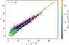Fig. 7. Scatter plot of ϵ vs $\sqrt{{ϵ}_c^2+v_{+}^2}$, with v+ = qX(μ) and ϵc = 2.2, coloured by mass. The residual scatter at fixed v+ is smaller than the range covered as v+ changes.

$$\begin{array}{c}\hfill \mathcal{C}=ϵ-\sqrt{{ϵ}_c^2+v_{+}^2}=ϵ-b\simeq 0\end{array}$$(29)

as the constraint. This assumption reproduces the asymptotic behaviour of the constraint at both large and small v₊, and automatically guarantees the positivity of all eigenvalues.

Regardless of its exact expression, the threshold depends implicitly on mass through the smoothing scale of the variables. Imposing the constraint therefore introduces a mass dependence in all pdfs, which were so far completely mass independent when expressed in terms of variables normalised by σ₀₂. In fact, if we define the conditional distribution

$$\begin{array}{c}\hfill p(\mathrm{variable}|\mathrm{halo}\mathrm{of}\mathrm{mass}M)\equiv p(\mathrm{variable}|\mathcal{C}=0),\end{array}$$(30)

where the variable could be any of ϵ/σ₀₂, b/σ₀₂ or q/σ₀₂, the constraint introduces an explicit dependence on mass through ϵ_c/σ₀₂(M). Comparing these conditional distributions with measurements in our mass-segregated samples provides further validation of our ansatz on the constraint. To do this comparison properly, however, we need to average over each mass range because each of our samples covers a broad range of masses. We describe this step below.

Before moving on, we note that the most appropriate expression to describe the measurement of a variable in a set of protohaloes of given mass should actually be

$$\begin{array}{c}\hfill p(\mathrm{variable}|\mathcal{C}=0,\mathrm{peak},1\mathrm{st}),\end{array}$$(31)

with the conditions including also the peak and first crossing constraint (that is, null gradient, negative-definite Hessian, and threshold not having been crossed on any larger scale). These conditions provide a more accurate description of protohaloes, introducing at the same time new variables that might correlate with the stochasticity in y (which we currently ignore). However, including these effects is more complicated, and the resulting expressions are not always analytical. For these reasons, we continued with the simpler equation (30).

3.1. Constrained q distribution and rescaling of variances

We noted above (histograms of Fig. 6, top panel) that the measured distribution of q/σ₀₂ is nearly mass-independent. We need to verify that this remains true for the predicted distribution in the presence of the mass-dependent constraint equation (29). Since 4q² = v₊² + 3v₋², the conditional distribution for q is

$$\begin{array}{c}\hfill p(q|\mathcal{C}=0)=\frac{\langle {\delta }_{\mathrm{D}}(q-\frac{1}{2}\sqrt{v_{+}^2+3v_{-}^2}){\delta }_{\mathrm{D}}(\mathcal{C})\rangle }{\langle {\delta }_{\mathrm{D}}(\mathcal{C})\rangle },\end{array}$$(32)

where ⟨…⟩ means that we averaged using equation (24) (in the numerator) or equation (25) (in the denominator). Note that the positivity condition is automatically implied by enforcing 𝒞 = 0.

The denominator of the expression above evaluates to

$$\begin{array}{c}\hfill \langle {\delta }_{\mathrm{D}}(\mathcal{C})\rangle =\frac{{\mathrm{e}}^{-{ϵ}_c^2/2}}{36\sqrt{\pi }}\sqrt{5(29-6\sqrt{6})};\end{array}$$(33)

thus, replacing ϵ_c → ϵ_c/σ₀₂(M) to reintroduce σ₀₂, it is exponentially mass dependent. However, the exponential cancels out with a similar term in the numerator, and we get

$$\begin{array}{cc}\hfill p(q|\mathcal{C}=0)& =\frac{{15}^2\sqrt{2}q{\mathrm{e}}^{-5q^2/2}}{\sqrt{(29-6\sqrt{6})}}{\displaystyle {\int }_q^{2q}}\mathrm{d}v\frac{{\mathrm{e}}^{-v^2/2}}{\sqrt{2\pi }}(v^2-q^2)\hfill \\ \hfill & =\frac{{15}^{2}q{\mathrm{e}}^{-5q^2/2}}{\sqrt{\pi (29-6\sqrt{6})}}[q({\mathrm{e}}^{-q^2/2}-2{\mathrm{e}}^{-2q^2})\hfill \\ \hfill & +\sqrt{\frac{\pi }{2}}(q^2-1)(\mathrm{erf}\left(\frac{q}{\sqrt{2}}\right)-\mathrm{erf}\left(\sqrt{2}q\right))],\hfill \end{array}$$(34)

where there is no dependence on ϵ_c, and thus no mass dependence left. This expression is numerically quite close to equation (22); in particular, it is closer to the dashed curve in Fig. 6 than to the histograms there. In other words, using a better model for the threshold does not fix the disagreement with the measured distribution of q for protohaloes.

We should not expect to find perfect agreement, however, since protohalo patches are not spherical, whereas our analysis implicitly assumed they are. This for instance changes the prediction of the variance. To account at least qualitatively for this, we rescaled σ₀₂ (the standard deviation of ϵ in spheres containing a given mass) by an ad hoc factor whose value we motivate elsewhere (see Padmanabhan & Subramanian 1993; Betancort-Rijo & López-Corredoira 2002; Lam & Sheth 2008, for earlier work). Here, we simply note that this factor should be greater than unity, to compensate for the fact that ϵ in the protohalo shapes is always larger than in the corresponding Lagrangian sphere (Musso & Sheth 2023). We also assumed for simplicity that this factor is the same for all masses. To fix its amplitude, we required that the distribution of q/σ_ϵ match equation (34) closely. Fig. 8 shows that setting σ_ϵ = 1.35 σ₀₂ provides a reasonably good agreement: the rescaled histograms are closer to the solid curve than to the dotted one. Presumably, some of the small differences that remain are due to approximating equation (31) with equation (30), and ignoring the stochasticity that allowed us to approximate equation (28) with equation (29).

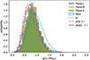Fig. 8. Distribution of q/(1.35σ02), the rescaling that provides the best match to equation (34) (purple solid line). Histograms show the measurements; dotted, dashed and solid curves show the distribution of random positions, those constrained to be positive definite, and those constrained to also have ϵ = b.

3.2. Testing the threshold ansatz

We tested if equation (29) is a useful parametrisation of the threshold for collapse by comparing the measured distributions of ϵ/σ₀₂ and b with the predicted conditional distribution. The latter can be expressed as

$$\begin{array}{c}\hfill p(b|\mathcal{C}=0)=\frac{{\int }_0^b\mathrm{d}{v}_{+}{\delta }_{\mathrm{D}}(b-\sqrt{{ϵ}_c^2+v_{+}^2})p(ϵ=b,v_{+})}{{\int }_0^{\infty }\mathrm{d}ϵ{\int }_0^{ϵ}\mathrm{d}{v}_{+}{\delta }_{\mathrm{D}}(ϵ-\sqrt{{ϵ}_c^2+v_{+}^2})p(ϵ,v_{+})};\end{array}$$(35)

Explicit calculation, using p(ϵ, v₊) from equation (25), yields

$$\begin{array}{c}\hfill p(b|\mathcal{C}=0)=\frac{18b{\mathrm{e}}^{-9v_{+}^2/8}}{\sqrt{\pi v_{+}^2}}\frac{{\mathrm{e}}^{-15v_{+}^2/8}-1+15v_{+}^2/8}{\sqrt{29-6\sqrt{6}}}{|}_{v_{+}^2=b^2-{ϵ}_c^2},\end{array}$$(36)

where 2b db = 2v₊ dv₊ is the reason why there is a b/v₊ factor in the expression above. Of course, this assumes that b ≥ ϵ_c, and p(b|𝒞 = 0) = 0 otherwise.

This distribution explicitly depends on ϵ_c, that is, after reintroducing σ₀₂, on ϵ_c/σ₀₂(M), so we must be careful when comparing it with measurements that span a range of masses. (This was not a concern for q/σ₀₂, for which there was no predicted mass dependence). To make a fair comparison, we averaged equation (36) over the same set of masses that contributed to the measurement. This average is

$$\begin{array}{c}\hfill p(b|[M_1,M2])=\frac{{\int }_{M_1}^{M_2}\mathrm{d}Mn(M)p(b|\mathcal{C}=0)}{{\int }_{M_1}^{M_2}\mathrm{d}Mn(M)},\end{array}$$(37)

where n(M) is the mass function. Ideally, we would like to predict n(M), rather than using the measured distribution. While a more careful derivation is the subject of work in progress, the plots that follow were made using the actual distribution of masses measured in each sample. We provide a simple estimate for n(M) motivated by an approach a la Press–Schechter in Appendix A.2.

With this in mind, we proceeded to a quantitative comparison. The filled histograms of Fig. 9 show the distribution of b in three of our protohalo samples, and the dashed step lines the measured distribution of ϵ (i.e. the same histograms as in Fig. 5). The similarity of the two sets of histograms proves that setting ϵ² = ϵ_c² + v₊² accounts for most of the scatter and is therefore a very good approximation for the threshold for halo formation.

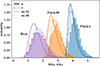Fig. 9. Distribution of $b=\sqrt{{ϵ}_c^2+v_{+}^2}/{\sigma }_{02}$ in the three mass bins (filled histograms). The dashed lines show the distribution of ϵ/σ02 (from Figure 5), the solid lines show equation (36) averaged over the measured distribution of σ02 values, and the dotted lines show equation (A.8).

The measured histograms are shifted to higher values of b/σ₀₂ (compared to the theory curves). In our discussion of q, we noted that rescaling σ₀₂ → 1.35σ₀₂ worked quite well; hence, it is natural to ask if this also works well here. Fig. 10 shows that it does. As further confirmation of the accuracy of this rescaling, Fig. 11 compares the distribution of b/1.35 measured in narrow mass bins directly with equation (36). We chose three mass intervals of (1 − 2)×10¹¹, (4 − 5)×10¹³ and (1 − 1.25)×10¹⁵ h⁻¹ M_⊙, corresponding to the lower end of Bice, Flora-S and Flora-L respectively. The bins are sufficiently narrow that no averaging over σ₀₂ values should be needed. Therefore, for the theory curves we use as ω_c the mean of ϵ_c/(1.35σ₀₂) in each narrow bin.

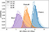Fig. 10. Weighted average of equation (36) (solid curves) with ϵc → ϵc/(1.35σ02), as described in the main text, providing an excellent description of the rescaled histograms of b/(1.35σ02) for all samples. The dotted curves show equation (A.8).

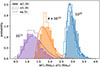Fig. 11. Distribution of b/(1.35σ02) (filled histograms) and ϵ/(1.35σ02) (empty dashed) in three narrow mass bins of mass 1011, 4 × 1013 and 1015 h−1 M⊙ (from left to right). The solid curves show equation (36).

The remarkable agreement with the filled histograms confirms that simply requiring the positivity of the eigenvalues, and imposing the approximate constraint ϵ² = ϵ_c² + v₊², gets very close to describing the correct distribution of v₊ (and thus of b) in protohaloes. In turn, b is a rather good approximation to the value of ϵ, and therefore to the collapse threshold of protohaloes. While a more careful calculation would require that we also impose the excursion set and peak constraints (see equation 31 and related discussion), we believe that the considerably simpler calculation discussed here (equations 29 and 30) captures most of the interesting physics.

4. Discussion and conclusions

We explored the statistical implications of two facts of dynamical origin that make protohaloes – the initial patches that are destined to become haloes – special locations: they must collapse along three axes, and they have to do so by today. Expressed in mathematical terms, these conditions are:

• (a)

  the energy shear u_ij is positive definite, so that all three axes of the protohalo collapse (Musso et al. 2024);

• (b)

  ϵ, the trace of u_ij, must exceed a critical value for the collapse to complete by the present day (Musso & Sheth 2021).

Both conditions are interesting in their own right.

The energy shear tensor u_ij (equation 1) measured at random positions in a Gaussian random field is a Gaussian random matrix, and its three rotational invariants (equation 4) are therefore uncorrelated with one another. However, in protohaloes they are strongly correlated (Fig. 2). We showed that the measured correlation pattern – in particular, the limiting values of some of these correlations (Figs. 2 and 3) – directly follows from the positive definiteness of the energy shear, that is from condition (a). We provided analytic expressions for the distributions of the three invariants, and their correlations, subject to these conditions (equations 21–23, and A.3–A.5 if one also requests ϵ > ϵ_c).

Previous work showed that the collapse threshold in ϵ is stochastic, with an absolute lower bound that we denoted ϵ_c. Fig. 2 shows that, for the protohaloes of haloes identified at z = 0, ϵ_c ≃ 2. Although condition (a) cannot explain the lower bound, the positivity requirement means that the excursion above this limit strongly correlates with the other rotational invariants (built out of differences of the eigenvalues). We verified that a parametrization of the stochasticity based on v₊ (equation 12) appears to be more efficient – that is, it has significantly less residual scatter – than one based on the rotational invariants q and μ (compare Figs. 2 and 4). In particular, ϵ in protohaloes is very close to $b=\sqrt{{ϵ}_c^2+v_{+}^2}$ (Fig. 7). Parametrising the threshold with this expression accounts for most of its stochasticity.

We then computed the conditional distribution of q given that ϵ equals the threshold. The result is rather insensitive to the constraint, and it matches the measured distributions well provided that one rescales σ₀₂ (the standard deviation of ϵ in spherical volumes) by a factor of 1.35 (Fig. 8). We argued that this rescaling can be attributed to the fact that protohaloes are not spherical. Computing it from first principles is the object of current work. The conditional distribution of b (equation 36), on the other hand, is very sensitive to the constraint, which makes it strongly mass dependent. However, the same variance rescaling brings the measurements of this quantity into good agreement with our (mass-dependent) predictions.

To summarise, we began our study with two main goals. One was the question of whether μ, the third invariant of the energy shear tensor, matters for protohaloes. Fig. 2 shows that it does, which has therefore potential implications for assembly bias. Our subsequent analysis suggests that a more efficient parametrisation of the physics of collapse uses v₊, a non-linear combination of the second and third invariants (q and μ) that is actually linear in the eigenvalues themselves (equation 13).

The second goal was to determine if the correlations between the invariants of the energy shear measured at protohalo positions (at random positions they are independent) can be understood as simply arising from the positivity of the eigenvalues. Here too the answer is yes, but with some subtleties. Our analysis suggests that triaxial collapse requires λ₃ ≥ 0, but collapse by today means ϵ ≥ 2. For very massive protohaloes, the dominant condition is the latter: in this regime, ϵ ∼ 2 with very little residual dependence on other rotational invariants. For smaller objects, however, which typically have ϵ ≫ 2, much of the correlation between ϵ and q or v₊ emerges from the constrained statistics, rather than being an additional physical requirement. The positivity condition is much simpler in the basis (ϵ, v₊, v₋) than in (ϵ, q, μ), which explains why parametrising the stochasticity of the threshold with v₊ is more efficient.

Our predictions are completely analytic and reasonably simple. This contrasts with many results on protohalo statistics, typically based on peak theory and first passage probabilities, which require rather involved calculations. These complications are indeed necessary when computing number densities, masses and correlation functions. However, a byproduct of our analysis is that they are not always required to predict the probability of secondary quantities in protohaloes. For these, conditioning on a sufficiently good model of the threshold is enough.

These results bring us closer to a first-principles derivation of the abundance of dark matter haloes and their properties. Whereas it is quite well established that haloes originate from sufficiently high peaks of the initial field smoothed on the corresponding mass scale, how tall these peaks should exactly be is a point under active discussion. Previous research has shown that the threshold is not the same for all haloes: it contains significant scatter. Accounting for this scatter is crucial to correctly predict when each halo virialised. Moreover, there is considerable interest in the role of additional variables on halo formation and clustering (sometimes called ‘assembly’ or ‘secondary’ bias), and which observable properties of the final halo they determine. We anticipate that some of the distributions of these secondary quantities, which we derived in Section 3, may be helpful in modelling these effects.

Three specific issues that still need to be addressed are:

• (i)

  the effect of non-sphericity of protohalo shapes on their statistics;

• (ii)

  the effect on the statistics of accounting for the fact that protohalo positions define a point process; and

• (iii)

  the exact relation between the value of ϵ and the time of virialisation.

About the first point, our work suggests that the main effect of initial non-sphericity is to rescale all variances. In a follow-up to Musso & Sheth (2023), who required protohalo shapes to maximise ϵ, we are in the process of showing why this rescaling takes place. In addition, now that we have a good model for the critical threshold (equation 28), we believe we are in a position to apply the technology of excursion set energy peaks theory (Musso & Sheth 2021) to address point (ii). This will allow us to quantify assembly or secondary bias effects as well (Sheth & Tormen 2004; Dalal et al. 2008; Musso & Sheth 2014; Lazeyras et al. 2017; Matsubara 2019; Lazeyras et al. 2023). It might also help us to improve models of shape bias for intrinsic alignments (Blazek et al. 2015; Vlah et al. 2020; Lee & Moon 2024; Maion et al. 2025)

As for point (iii), we note that a halo identified at z = 0 may have virialised at an earlier time: halo finders do not usually make this distinction. Since in first approximation the evolution of the inertial radius follows spherical collapse, where the final time depends on the initial energy, the uncertainty in the virialisation time will add to the stochasticity in the value of ϵ (similarly to Borzyszkowski et al. 2014). Much of this stochasticity, as shown in this work, is described by v₊: when v₊ is large then so is ϵ, implying early virialisation. Moreover, ϵ ∼ v₊ means that λ₃ ∼ 0: these objects represent the transition between a protohalo and a protofilament (Hanami 2001; Cadiou et al. 2020; Salvador-Solé & Manrique 2021), and can be associated with haloes that stopped accreting before the time of identification due to tidal stripping (as found in simulations by Borzyszkowski et al. 2017). There is however also a residual scatter in ϵ at fixed v₊, which might be related to how virialisation depends on the slope of the initial profile. We hope to quantify this effect in future work.

To obtain a more reliable estimate of the virialisation time in an anisotropic environment (large v₊), we may consider perturbative corrections to spherical collapse. These corrections naturally scale like q²/ϵ². Our analysis suggests that this ratio cannot exceed unity, which helps us to keep the perturbative treatment under control. Physically, this can be interpreted as reflecting the fact that the evolution cannot deviate too much from spherical collapse, even for arbitrary shapes, simply because the protohalo patch must end up in a very small region in order to create a high enough density. This is what makes protohaloes special locations.

Finally, our goal is to predict where haloes form in the initial field. Recent machine-learning based work aims to predict where they occur in the evolved field (Pandey et al. 2024). We hope that our work will be useful to train these algorithms to make predictions from the initial field.

Data availability

The simulation data and the post-processing quantities used in this work can be shared on reasonable request to the authors.

Acknowledgments

We are grateful to the anonymous referee for a helpful report. Thanks to G. Despali for sharing the data from the SBARBINE simulations, and to the organisers and participants of the 2023 KITP Cosmic Web workshop. Our visit to KITP was supported by the National Science Foundation under PHY-1748958. We are grateful to the EAIFR, Kigali and the ICTP, Trieste for their hospitality in summer 2024, when this work was completed. Marcello Musso acknowledges support from grants PID2021-122938NB-I00, PID2024-158938NBI00 and CNS2024-154286 funded by MICIU/AEI/10.13039/501100011033 and by “ERDF A way of making Europe”, and SA097P24 funded by Junta de Castilla y León.

References

Appendix A: Statistics for a range of masses

We discuss a simple model for the statistics when the sample includes objects more massive than a given threshold. The approach is similar to that of Press & Schechter (1974), which is known to not be very accurate – in particular, it does not account for the fact that haloes define a point process. Nevertheless, we believe it provides some insight.

A.1. Simple threshold: ϵ = ϵ_c

Integrating over masses above a threshold is like integrating σ₀₂ from 0 to an upper limit. Since the statistics depend on ϵ_c/σ₀₂, this is like integrating ϵ_c from a lower limit to infinity.

Hence, as a warm up, consider simply requiring ϵ ≥ ϵ_c. To quantify how the distribution of ϵ, q and μ are modified, we first define the new normalisation

$$\begin{array}{c}\hfill p(+{ϵ}_c)\equiv p({\lambda }_3\le 0,ϵ>{ϵ}_c)=p(+){\displaystyle {\int }_{{ϵ}_c}^{\infty }}dϵp(ϵ|+).\end{array}$$(A.1)

Although no analytical expression for p(+ϵ_c) exists, a simple and reasonably accurate approximation is

$$\begin{array}{cc}\hfill p(+{ϵ}_c)& \simeq \frac{1}{4}\mathrm{erfc}\left(\frac{{ϵ}_c}{\sqrt{2}{\sigma }_{02}}\right)[1+\mathrm{erf}\left(\frac{{ϵ}_c}{\sqrt{2}{\sigma }_{02}}\right)]\hfill \\ \hfill & -\frac{\sqrt{5}}{3\pi }{\mathrm{e}}^{-9{ϵ}_c^2/8{\sigma }_{02}^2}+\frac{\pi -2arctan(\sqrt{5})}{4\pi }{\mathrm{e}}^{-3{ϵ}_c^2/2{\sigma }_{02}^2},\hfill \end{array}$$(A.2)

which captures the correct asymptotic behaviour for small and large σ₀₂ (large and small masses) and deviates from the numerical solution by less than 1.8% over the entire positive axis.

Equations (21), (22) and (23) are changed to

$$\begin{array}{cc}\hfill p(ϵ|+{ϵ}_c)& =\mathrm{\Theta }(ϵ-{ϵ}_c)p(ϵ|+)\frac{p(+)}{p(+{ϵ}_c)},\hfill \end{array}$$(A.3)

$$\begin{array}{cc}\hfill p(q|+{ϵ}_c)& =\frac{\chi (q)}{p(+{ϵ}_c)}[{\displaystyle {\int }_{q_{\min 2}}^{\infty }}dϵp(ϵ)\hfill \\ \hfill & +{\displaystyle {\int }_{q_{\min 1}}^{q_{\min 2}}}dϵp(ϵ)\frac{(ϵ/2q)({ϵ}^2/q^2-3)+1}{2}]\hfill \\ \hfill & =\frac{\chi (q)}{4p(+{ϵ}_c)}[\mathrm{erfc}\left(\frac{q_{\min 1}}{\sqrt{2}}\right)+\mathrm{erfc}\left(\frac{q_{\min 2}}{\sqrt{2}}\right)\hfill \\ \hfill & -\frac{{\mathrm{e}}^{-q_{\min 2}^2/2}}{\sqrt{2\pi }}\frac{(q_{\min 2}^2+2-3q^2)}{q^3}\hfill \\ \hfill & +\frac{{\mathrm{e}}^{-q_{\min 1}^2/2}}{\sqrt{2\pi }}\frac{(q_{\min 1}^2+2-3q^2)}{q^3}]\hfill \end{array}$$(A.4)

where q_minn ≡ max(ϵ_c/σ₀₂, nq), and

$$\begin{array}{cc}\hfill p(\mu |+{ϵ}_c)& =\frac{1}{2p(+{ϵ}_c)}{\displaystyle {\int }_{{ϵ}_c}^{\infty }}\mathrm{d}ϵp(ϵ){\displaystyle {\int }_0^{ϵ/X}}\mathrm{d}q\chi (q)\hfill \\ \hfill & ={\displaystyle {\int }_{{ϵ}_c}^{\infty }}\mathrm{d}ϵ\frac{p(ϵ)}{2p(+{ϵ}_c)}[\mathrm{erf}\left(\sqrt{\frac{5}{2}}\frac{ϵ}{X}\right)\hfill \\ \hfill & -\sqrt{\frac{10}{\pi }}ϵ\frac{5{ϵ}^2+3X^2}{3X^3}{\mathrm{e}}^{-5{ϵ}^2/2X^2}].\hfill \end{array}$$(A.5)

The last integral does not have an analytical expression, but an approximation accurate to better than 1.5% is

$$\begin{array}{cc}\hfill p(\mu |+{ϵ}_c)& \simeq \frac{1}{p(+{ϵ}_c)}[\frac{1}{8}(\mathrm{erf}\left(\frac{{\omega }_c}{\sqrt{2}}\right)+1)\mathrm{erfc}\left(\frac{{\omega }_c}{\sqrt{2}}\right)\hfill \\ \hfill & +(\frac{arctan(\sqrt{5}/X)}{2\pi }-\frac{1}{8}){\mathrm{e}}^{-(X^2+5){\omega }_c^2/4X}].\hfill \end{array}$$(A.6)

Massive objects correspond to the ϵ_c/σ₀₂ ≫ 1 limit, for which $p(+{ϵ}_c)\simeq \frac{1}{2}\mathrm{erfc}({ϵ}_c/\sqrt{2}{\sigma }_{02})$ and q_min1 = q_min2 = ϵ_c/σ₀₂. Therefore, only the first term of equation (22) contributes and tends to χ(q) of Eq. (19) (dotted curve in Fig. 6). In contrast, at small masses the limits of the integrals in Eq. (22) are modified only when q ≤ 2 (i.e. not significantly). As a result, lower mass haloes are better described by Eq. (22) (dashed curve in Fig. 6).

These limiting cases can also be understood by looking at Fig. 2 which shows the two cuts explicitly: the dashed line showing ϵ = q and the obvious floor at ϵ = 2. Most lower mass haloes tend to have large q, so they are less affected by the ϵ > 2 floor: the ϵ > q cut matters much more. However, massive haloes tend to have small q, so the ϵ > 2 floor is the only relevant cut. In a Gaussian field, the distribution of q is uncorrelated with ϵ. This is modified by the ϵ = q cut, but, since this cut is irrelevant for the massive haloes, their distribution is not given by Eq. (22); instead, it should be much closer to Eq. (19). Fig. 6 shows that the distribution of massive haloes is indeed shifted towards larger values, as expected.

By this argument, one would expect the distribution of μ for massive haloes to be closer to that for unconstrained positions (uniform on [ − 1, 1]); this is in qualitative agreement with the trend in the bottom panel of Fig. 6, where the largest mass objects (green) are closest to being uniformly distributed.

A.2. More realistic threshold: $ϵ=\sqrt{{ϵ}_c^2+v_{+}^2}$

Now suppose the threshold is given by equation (28) of the main text (and the extra variable y is ignored). Integrating over all masses above some minimum means we now want $\sqrt{{ϵ}^2-v_{+}^2}/{\sigma }_{02}>{\omega }_c$, or equivalently $v_{+}/{\sigma }_{02}<\sqrt{{\omega }^2-{\omega }_c^2}$. The resulting distribution is then

$$\begin{array}{c}\hfill p(b|\mathcal{C}>0)\propto {\displaystyle {\int }_0^{\sqrt{b^2-{\omega }_c^2}}}\mathrm{d}{v}_{+}p(ϵ=b,v_{+}),\end{array}$$(A.7)

where the integral is analytical and is easily seen to be equal to ${\mathrm{e}}^{-{\omega }_c^2/2}p(\sqrt{b^2-{\omega }_c^2}|+)p(+)$. Normalising to unity, we get

$$\begin{array}{c}\hfill p(b|\mathcal{C}>0)=\frac{p(ϵ=\sqrt{b^2-{\omega }_c^2}|+)}{N({\omega }_c)},\end{array}$$(A.8)

where N(ω_c) is the integral of the numerator over b > ω_c. Changing variables from b to $\sqrt{b^2-{\omega }_c^2}$, the normalisation becomes

$$\begin{array}{c}\hfill N({\omega }_c)={\displaystyle {\int }_0^{+\infty }}\mathrm{d}ϵ\frac{ϵ}{\sqrt{{ϵ}^2+{\omega }_c^2}}p(ϵ|+);\end{array}$$(A.9)

this integral has no known analytical solution, but can be approximated by Taylor-expanding the fraction $ϵ/\sqrt{{ϵ}^2+{\omega }_c^2}$ around the conditional mean ⟨ϵ|+⟩ ≃ 1.663. At second order, this gives

$$\begin{array}{c}\hfill N({\omega }_c)\simeq \frac{\langle ϵ|+\rangle }{\sqrt{{\langle ϵ|+\rangle }^2+{\omega }_c^2}}[1-\frac{3\mathrm{Var}(ϵ|+)}{{({\langle ϵ|+\rangle }^2+{\omega }_c^2)}^2}\frac{{\omega }_c^2}{2}],\end{array}$$(A.10)

where Var(ϵ|+)≃0.3010. This approximation is asymptotically correct for both large and small ω_c (in which limits one gets ⟨ϵ|+⟩/ω_c and 1 respectively), and numerically accurate to less than 0.4% everywhere. The dotted curves in Fig. 9 show equation (A.8). While the agreement with the measurements is not compelling, as we noted above, this is only a crude estimate. A better estimate would include the peak and first-crossing constraints, and the corresponding Jacobians: the Hessian determinant and the slope of the excursion set (Musso & Sheth 2021). This is the subject of ongoing work.

All Figures

	Fig. 1. Ratio of traceless eigenvalues to q/3 as a function of μ (equation 7). Also shown (dashed line) is the function X(μ) defined in equation (10), marking the lower limit of ϵ/q.
In the text

Fig. 2. Top panel: Correlation between the three rotational invariants of protohaloes: energy overdensity ϵ, the traceless energy shear q, and μ (see equation 4). The colour displays the value of μ. The dashed lines show ϵ = nq for n = {1, 4/3, 5/3, 2} (from bottom to top), corresponding to the minimum value of ϵ for μ = {1, 0.815, 0.185, −1} whenever the energy shear tensor is positive definite – as shown by equation (10). Bottom panel: Expected distribution of ϵ − q and μ if protohaloes where centred on random locations constrained to have the measured values of ϵ (typically ϵ ≳ 2).

In the text

	Fig. 3. Correlation of ϵ (top panel) and q/ϵ (bottom) with μ for protohaloes, coloured by log10(M/h−1 M⊙). The dashed line in the bottom panel shows the upper limit given by (the inverse of) equation (10).
In the text

	Fig. 4. Correlation of ϵ with v+, with colours showing the value of v−/v+. The scatter is significantly narrower than in Figure 2, especially at higher values, and there is no residual correlation signal with v−/v+. Dashed line shows the theoretical lower limit ϵ = v+, and solid line shows $\sqrt{{ϵ}_c^2+v_{+}^2}$ with ϵc = 2.2.
In the text

	Fig. 5. Distribution of trace ϵ/σ02 for a few ranges in halo mass (histograms). The dotted curve shows the expected (zero-mean, unit variance Gaussian) distribution at unconstrained positions; the dashed curve, at positions with λ3 ≥ 0 (Eq. 21). More massive haloes have larger ϵ/σ02, but the distribution around the mean is approximately independent of mass.
In the text

	Fig. 6. Distribution of traceless shear q/σ02 (top) and μ (bottom). The dotted curves show the expected distributions at unconstrained positions; the dashed ones, at positions with λ3 ≥ 0 (equations 22 and 23). Whereas q/σ02 is approximately the same for all masses, μ is closer to uniform as mass increases.
In the text

	Fig. 7. Scatter plot of ϵ vs $\sqrt{{ϵ}_c^2+v_{+}^2}$, with v+ = qX(μ) and ϵc = 2.2, coloured by mass. The residual scatter at fixed v+ is smaller than the range covered as v+ changes.
In the text

	Fig. 8. Distribution of q/(1.35σ02), the rescaling that provides the best match to equation (34) (purple solid line). Histograms show the measurements; dotted, dashed and solid curves show the distribution of random positions, those constrained to be positive definite, and those constrained to also have ϵ = b.
In the text

	Fig. 9. Distribution of $b=\sqrt{{ϵ}_c^2+v_{+}^2}/{\sigma }_{02}$ in the three mass bins (filled histograms). The dashed lines show the distribution of ϵ/σ02 (from Figure 5), the solid lines show equation (36) averaged over the measured distribution of σ02 values, and the dotted lines show equation (A.8).
In the text

	Fig. 10. Weighted average of equation (36) (solid curves) with ϵc → ϵc/(1.35σ02), as described in the main text, providing an excellent description of the rescaled histograms of b/(1.35σ02) for all samples. The dotted curves show equation (A.8).
In the text

	Fig. 11. Distribution of b/(1.35σ02) (filled histograms) and ϵ/(1.35σ02) (empty dashed) in three narrow mass bins of mass 1011, 4 × 1013 and 1015 h−1 M⊙ (from left to right). The solid curves show equation (36).
In the text

References

- Bardeen, J. M., Bond, J. R., Kaiser, N., & Szalay, A. S. 1986, ApJ, 304, 15 [Google Scholar]
- Betancort-Rijo, J., & López-Corredoira, M. 2002, ApJ, 566, 623 [NASA ADS] [CrossRef] [Google Scholar]
- Blazek, J., Vlah, Z., & Seljak, U. 2015, JCAP, 08, 015 [CrossRef] [Google Scholar]
- Bond, J. R., & Myers, S. T. 1996, ApJS, 103, 1 [NASA ADS] [CrossRef] [Google Scholar]
- Borzyszkowski, M., Ludlow, A. D., & Porciani, C. 2014, MNRAS, 445, 4124 [Google Scholar]
- Borzyszkowski, M., Porciani, C., Romano-Diaz, E., & Garaldi, E. 2017, MNRAS, 469, 594 [NASA ADS] [CrossRef] [Google Scholar]
- Cadiou, C., Pichon, C., Codis, S., et al. 2020, MNRAS, 496, 4787 [Google Scholar]
- Castorina, E., Paranjape, A., Hahn, O., & Sheth, R. K. 2016, ArXiv e-prints [arXiv:1611.03619] [Google Scholar]
- Dalal, N., White, M., Bond, J. R., & Shirokov, A. 2008, ApJ, 687, 12 [NASA ADS] [CrossRef] [Google Scholar]
- Desjacques, V. 2013, Phys. Rev. D, 87, 043505 [Google Scholar]
- Despali, G., Tormen, G., & Sheth, R. K. 2013, MNRAS, 431, 1143 [NASA ADS] [CrossRef] [Google Scholar]
- Despali, G., Giocoli, C., Angulo, R. E., et al. 2016, MNRAS, 456, 2486 [NASA ADS] [CrossRef] [Google Scholar]
- Doroshkevich, A. G. 1970, Astrophysics, 6, 320 [Google Scholar]
- Gunn, J. E., & Gott, J. R. 1972, ApJ, 176, 1 [NASA ADS] [CrossRef] [Google Scholar]
- Hanami, H. 2001, MNRAS, 327, 721 [NASA ADS] [CrossRef] [Google Scholar]
- Lam, T. Y., & Sheth, R. K. 2008, MNRAS, 386, 407 [Google Scholar]
- Lazeyras, T., & Schmidt, F. 2018, JCAP, 2018, 008 [CrossRef] [Google Scholar]
- Lazeyras, T., Musso, M., & Desjacques, V. 2016, Phys. Rev. D, 93, 063007 [Google Scholar]
- Lazeyras, T., Musso, M., & Schmidt, F. 2017, JCAP, 2017, 059 [Google Scholar]
- Lazeyras, T., Barreira, A., Schmidt, F., & Desjacques, V. 2023, JCAP, 2023, 023 [CrossRef] [Google Scholar]
- Lee, J., & Moon, J.-S. 2024, JCAP, 10, 102 [Google Scholar]
- Ludlow, A. D., Borzyszkowski, M., & Porciani, C. 2014, MNRAS, 445, 4110 [NASA ADS] [CrossRef] [Google Scholar]
- Maion, F., Stücker, J., & Angulo, R. E. 2025, A&A, 699, A271 [NASA ADS] [CrossRef] [EDP Sciences] [Google Scholar]
- Matsubara, T. 2019, Phys. Rev. D, 100, 083504 [Google Scholar]
- Modi, C., Castorina, E., & Seljak, U. 2017, MNRAS, 472, 3959 [Google Scholar]
- Musso, M., & Sheth, R. K. 2014, MNRAS, 438, 2683 [Google Scholar]
- Musso, M., & Sheth, R. K. 2021, MNRAS, 508, 3634 [NASA ADS] [CrossRef] [Google Scholar]
- Musso, M., & Sheth, R. K. 2023, MNRAS, 523, L4 [NASA ADS] [CrossRef] [Google Scholar]
- Musso, M., Despali, G., & Sheth, R. K. 2024, MNRAS, 523, L4 [Google Scholar]
- Padmanabhan, T., & Subramanian, K. 1993, ApJ, 410, 482 [Google Scholar]
- Pandey, S., Lanusse, F., Modi, C., & Wandelt, B. D. 2024, 41st International Conference on Machine Learning [Google Scholar]
- Press, W. H., & Schechter, P. 1974, ApJ, 187, 425 [Google Scholar]
- Salvador-Solé, E., & Manrique, A. 2021, ApJ, 914, 141 [Google Scholar]
- Sandvik, H. B., Möller, O., Lee, J., & White, S. D. M. 2007, MNRAS, 377, 234 [NASA ADS] [CrossRef] [Google Scholar]
- Sheth, R. K., & Tormen, G. 2002, MNRAS, 329, 61 [Google Scholar]
- Sheth, R. K., & Tormen, G. 2004, MNRAS, 350, 1385 [NASA ADS] [CrossRef] [Google Scholar]
- Sheth, R. K., Mo, H., & Tormen, G. 2001, MNRAS, 323, 1 [NASA ADS] [CrossRef] [Google Scholar]
- Sheth, R. K., Chan, K. C., & Scoccimarro, R. 2013, Phys. Rev. D, 87, 083002 [NASA ADS] [CrossRef] [Google Scholar]
- van de Weygaert, R., & Bertschinger, E. 1996, MNRAS, 281, 84 [NASA ADS] [CrossRef] [Google Scholar]
- Vlah, Z., Chisari, N. E., & Schmidt, F. 2020, JCAP, 01, 025 [Google Scholar]