| Issue |
A&A
Volume 707, March 2026
|
|
|---|---|---|
| Article Number | A37 | |
| Number of page(s) | 11 | |
| Section | The Sun and the Heliosphere | |
| DOI | https://doi.org/10.1051/0004-6361/202555775 | |
| Published online | 25 February 2026 | |
Characterisation of in situ signatures of coronal mass ejections interacting with high-speed streams
1
University of Zagreb, Faculty of Geodesy, Hvar Observatory 10000 Zagreb, Croatia
2
Institut de Recherche en Astrophysique et Planétologie (IRAP) 31400 Toulouse, France
3
Centre National d’Etudes Spatiales (CNES) 31400 Toulouse, France
4
Institute of Physics, University of Graz Universitätsplatz 5 8010 Graz, Austria
★ Corresponding author: This email address is being protected from spambots. You need JavaScript enabled to view it.
Received:
2
June
2025
Accepted:
28
December
2025
Abstract
Aims. Interactions between coronal mass ejection (CMEs) and high-speed streams (HSSs) have the capacity to alter their plasma and magnetic field properties. The properties of such interactions are expected to be encoded in the in situ plasma and magnetic field observations. To characterise the properties of these interactions, we aim to analyse the in situ signatures of 28 interplanetary coronal mass ejections (ICMEs) interacting with high-speed streams (HSS) at 1 AU between 2010 and 2018.
Methods. We analysed the ICME velocity profiles, the duration of the sheath and magnetic obstacle (MO), and the distortion of the MO, as well as search for the signatures of the reconnection exhausts. We found twenty events where the ICME was located in front of the HSS and eight where it was behind. Statistical analyses were performed separately for these two classes of interactions.
Results. We find that ICMEs interacting with an HSS generally show distinct speed profiles for cases where an HSS is in front and behind. We find that for HSS in front cases, the formation of the sheath is hindered, and the duration of MO seems to be shorter with a lower average magnetic field magnitude. We find that HSSs catching up to ICMEs tend to compress and accelerate them from the back, whereas HSSs in front of ICMEs do not significantly alter the typical speed expansion profiles. Although we find reconnection exhaust signatures in about 30% events, we do not find significant evidence of the distortion of the internal magnetic structure.
Conclusions. Our results indicate that interaction with an HSS does not significantly influence the ICME internal magnetic structure. However, it might significantly influence its kinematics.
Key words: Sun: coronal mass ejections (CMEs) / Sun: heliosphere / solar wind
© The Authors 2026
 Open Access article, published by EDP Sciences, under the terms of the Creative Commons Attribution License (https://creativecommons.org/licenses/by/4.0), which permits unrestricted use, distribution, and reproduction in any medium, provided the original work is properly cited.
This article is published in open access under the Subscribe to Open model. This email address is being protected from spambots. You need JavaScript enabled to view it. to support open access publication.
1. Introduction
Coronal mass ejections (CMEs) and high-speed streams (HSSs) are among the most prevalent drivers of space weather phenomena. In brief, CMEs are large expulsions of highly magnetised plasma from the Sun’s corona, while high-speed streams (HSSs) are fast-moving solar wind originating from coronal holes (CHs). Interplanetary extensions of CMEs (ICMEs) directed towards Earth can interact with the magnetosphere and cause severe geomagnetic storms (e.g. Temmer 2021). HSSs and their associated stream interaction regions (SIRs), where the fast solar wind interacts with slow ambient wind during propagation). Although HSSs are generally less geoeffective than ICMEs, they can also cause severe geomagnetic disturbances (e.g. Richardson 2006).
These two dynamic transients can encounter each other as they evolve through interplanetary space, often leading to interactions that amplify their individual magnetic field and plasma characteristics. Case studies have shown that CME-HSS interactions may add to the CME’s complexity (Heinemann et al. 2019a; Dumbović et al. 2019; Scolini et al. 2022). In a case study, Winslow et al. (2021) found that even though the CME interacting with HSS did not undergo significant alterations to its magnetic topology, there were clear enhancements in plasma velocity and density, indicating compression. Kay et al. (2022) found that HSS-CME interaction may produce large changes in the sheath. He et al. (2018) found that even a stealth CME, which is typically not geoeffective owing to its typically low velocity and weak magnetic field, produces a G2 magnetic storm with a DST minimum of −104 nT when the CME was caught in the compression region of an HSS. In a statistical study, Heinemann et al. (2024) found that the interaction of slow ICMEs and faster HSS may lead to substantial geoeffective impact in comparison to SIR storm events. However, although there is plenty of evidence that an HSS might have the ability to alter the properties of ICMEs, a statistical study that would qualify and quantify the effects is still lacking.
Another aspect of CME-HSS interaction that has not been systematically studied is the possible erosion of the CME through CME-HSS interaction; namely, as CMEs traverse the heliosphere, they can also undergo magnetic reconnection with the ambient magnetic field. This interaction can significantly erode the flux rope structure, affecting the complexity and strength of the magnetic field inside a CME (e.g. Dasso et al. 2007). A statistical study from Ruffenach et al. (2015), Pal et al. (2021) showed that the erosion effects could happen roughly equally for the front and rear parts of the CME, with an average of 40% of the azimuthal flux eroding. Non-interacting ICMEs show a high correlation between the magnetic field strength and plasma velocity. However, ICMEs interacting with solar wind structures and altering their complexity lose this correlation, indicating that interaction can randomise their average internal properties (Scolini et al. 2022).
This study is aimed at statistically quantifying and qualifying CME-HSS interactions observed near Earth in situ by analysing 28 ICMEs observed at 1 AU between 2010 and 2018. We investigate their physical characteristics, focussing on their associated plasma and magnetic field properties, as well as searching for signatures of reconnection exhausts.
2. Data and method
To find ICME-HSS interaction events, we use the CME-ICME list in the vicinity of coronal holes (CH) compiled by Karuppiah et al. (2024) and the CH-HSS list compiled by Heinemann et al. (2019b). We analysed plasma and magnetic field measurements around these events using in situ magnetic field and plasma data from WIND and Advanced Composition Explorer (ACE) (Acuña et al. 1995; Stone et al. 1998), compiled in the OMNI database (King & Papitashvili 2020). To characterise the interaction signatures, we analysed two distinct interaction scenarios: the first being the cases where the ICME arrives first at 1 AU, with a trailing HSS (hereafter, HSS behind) and the second being the cases where the HSS arrives first with a trailing ICME (hereafter, HSS in front).
Detections of ICMEs in interplanetary space are carried out on the basis of their characteristic signatures that include some or all of the following properties: a compressed, heated, and turbulent sheath region, followed by increased and smooth rotating magnetic field components, low plasma beta and low plasma density (Burlaga et al. 1981), and a lower than expected plasma temperature, which is an estimate for the proton temperature calculated from the proton velocity (Lopez 1987). The events that satisfy all of these signatures are typically referred to as magnetic clouds and comprise one-third of the observed ICMEs. The rest (where only partial signatures are present) are classified as magnetic ejecta or magnetic obstacles (MOs) (Richardson & Cane 2010; Winslow et al. 2016; Nieves-Chinchilla et al. 2018). We use the term MO to refer to the events analysed in this work.
An HSS is identified as a region of increased plasma velocity and temperature, coupled with reduced density. The stream interface (SI) is determined by locating a change in azimuthal flow angle, dip in plasma density, increase in plasma temperature, and increase of velocity profile, similarly as the approach in Dumbović et al. (2022). We used the plasma entropy, Sp, as an additional indicator for identifying HSS. We defined a plasma entropy threshold of  , where Tp and Np are plasma temperature and density respectively) of 4 eV cm2. We used any result above this as an indicator of CH plasma (e.g. Xu & Borovsky 2015). We identified an event as an MO for the purposes of our analysis when at all three of the following criteria were observed:
-
smooth and rotating magnetic field;
-
plasma beta lower than 1;
-
proton temperature lower than the expected temperature.
We cross-checked our ICME identification with ICME lists by Richardson (2018) and Nieves-Chinchilla et al. (2019) and relied on their ICME borders as a first approximation. We also note that not all of our events show consistent signatures of MO (e.g. the proton temperature being lower than the expected temperature) throughout the period of interest, as the interaction can alter certain properties at the local level (e.g. heating and compressing parts of MO), causing anomalous signatures. Furthermore, as interpreting the magnetic field’s change at the boundary is often difficult, to ensure consistency in our analysis, we refined the boundary definition, choosing the plasma beta (β) and magnetic field behaviour as indicators for the start and end of the MO. We define the boundary as the point closest to a clearly discernible, smoothly rotating magnetic field where the plasma beta rises above 1. We found 28 ICME-HSS interactions (figures provided in figshare1). Out of these, there are 8 cases where the HSS is in front and 20 where the HSS is behind (see Fig. 1 for examples). Out of these identified events, 23 appear in Richardson (2018), 21 appear in Nieves-Chinchilla et al. (2019), and 19 are catalogued in both, with three events not catalogued in either.
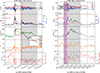 |
Fig. 1. Plots showing examples of ICME-HSS interaction and HSS-ICME interaction. Top panel: Magnetic field components in GSE coordinates. Second panel: Proton temperature (black) over plotted with the expected plasma temperature (red) and plasma density (blue). Third panel: Plasma velocity. Fourth panel: Plasma beta. Fifth panel: Plasma entropy (grey) and azimuthal (longitudinal) plasma flow angle (red). The horizontal red line in panel four marks the value one for plasma beta, the horizontal red line in panel four marks the value four for plasma entropy, while the horizontal black line marks zero for azimuthal flow angle. The shaded grey regions show the HSS (from the stream interface to the end), whereas the vertical black lines mark the start and end of the MO. The shaded brown region in the left panels marks the disturbed region (the zoomed-in plot highlights the same with the front and back of the MO marked with red and blue arrows, respectively. For more details, see the main text). The shaded purple region in the right panels marks the compression region + SIR. |
In the following sections, we use our sample to explore the statistical properties of the plasma and magnetic field associated with ICMEs. We begin by describing the general characteristics of ICMEs, such as the duration of the sheath and magnetic obstacle (MO), as well as the average magnetic field strength and velocity within the MO. Next, we investigate how the kinematics and plasma properties are influenced by the interaction with the HSS by quantifying the disturbance inside the MO (see Section 2.1). This is followed by an analysis of the velocity profiles inside the MO and their slopes (see Section 2.2), along with comparisons to the average velocities of HSSs and ICMEs. To better understand the magnetic field signatures of these interactions, we examine distortions in the magnetic field (Section 2.3) and look for signs of magnetic reconnection (Section 2.4) in the interaction region. Additionally, to combat the relatively small sample size, we use the Student’s t-test (STUDENT 1908) and Mann-Whitney-U test (Mann & Whitney 1947) to assess the statistical significance of the observed characteristics.
2.1. The fraction of the kinematically disturbed part of MO
We consider a part of the MO to be disturbed when its in situ speed profile begins to clearly deviate from the anticipated smooth, linearly decreasing trend. To quantify this, we manually identified the point on the velocity profile where this deviation starts and present it as a percentage of the MO’s total duration. This percentage gives us a simple, intuitive scale:
-
a perfectly behaved MO that follows the expected linear trend throughout is recorded as 0% distortion;
-
an MO that starts deviating halfway through is assigned 50% distortion;
-
an MO showing a fully non-linear profile (e.g. a constantly increasing speed) is recorded as 100% disturbed.
As the example in Figure 1 illustrates, because we do not have a single, rigid quantitative rule for where the disturbance begins, this identification process remains somewhat subjective. However, this percentage can serve as an indicator of the overall extent to which the MO’s expected motion was kinematically disrupted during the interaction.
2.2. Speed profiles
To quantify the amount of distortion the ICME underwent, we analysed the speed profiles. An undisturbed ICME typically shows a monotonically decreasing flow speed profile, which is a direct consequence of the expansion of MO (e.g. Kilpua et al. 2017; Gulisano et al. 2010). We hypothesise that the nature and duration of the interaction may influence the speed profiles, causing deviations from the typical expansion pattern. Figure 2 illustrates the hypothesised variations in speed profiles under no interaction and different interaction scenarios:
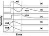 |
Fig. 2. Sketch showing different hypothesised speed profiles inside MO: a) undisturbed MO; b) slower CME is accelerated by the faster HSS behind for a shorter time period; c) lower CME is accelerated by the faster HSS behind for a longer time period; d) CME faster than the HSS is catching up with it; e) CME moving with the HSS. For details, see the main text. |
-
(a)
undisturbed ICME having a typical linearly decreasing speed profile;
-
(b)
a slower ICME is pushed and accelerated by the faster HSS behind for a shorter period, inhibiting or preventing expansion in the rear, resulting in a U-shape speed profile;
-
(c)
a slower ICME pushed and accelerated by the faster HSS behind for a longer period, resulting in a fully flat, no-expansion profile;
-
(d)
an ICME faster than the HSS is catching up with it, generating a sheath in front, having a typical monotonically decreasing speed profile;
-
(e)
an ICME moving with the HSS, not generating a sheath, and having a typical monotonically decreasing speed profile.
We could expect cases where the HSS is behind the ICME to show imprints of acceleration (and hindered expansion) in the rear part of the MO. Similarly, for cases where the HSS interaction occurs in front of the ICME, depending on the speed difference between the HSS and ICME, we might expect to see less prominent sheaths and minimal change in the general expansion profile. We note that there may also be a specific case of ICME moving within the HSS. The left panels of Fig. 1 show an example of an ICME compressed by the trailing HSS (case b) and the right panels show the ICME locally engulfed by an HSS (case e, where we observe the same HSS in front and behind the ICME). We note that by locally engulfed, we considered an ICME observed in situ with HSS originating from the same coronal hole preceding and trailing the ICME (e.g. Heinemann et al. 2019b). We see that the velocity profile for the first case shows no expansion traits, while the latter case shows a clear sign of expansion in the velocity profile during the interaction.
To test events for these scenarios, we analysed the speed profiles using several different approaches. First, we analysed the slope of the flow speed profile. Based on the total duration of the MO, it is divided into two parts for each event: front and back. The front part is defined as the region between the start of the MO and half of its total duration, while the back part is defined as the region between half of the total duration and the end of the MO (see 1). The slopes were calculated and analysed separately for these two regions.
Next, we used the superposed epoch analysis (SEA, e.g. Chree 1913) to analyse the velocity profiles for events with HSS in front and behind the ICME. We chose the ICME-HSS boundary as the zero epoch. For HSS behind cases, the left of the zero epoch is normalised to the MO duration and the right of the zero epoch is normalised to the period until the maximum speed of HSS. For HSS in front cases, the data left of the zero epoch is normalised to the period between the SI and the zero epoch, and the data right of the zero epoch is normalised to the duration of the MO. We omitted outliers showing significant distortions in speed profiles to better extract general characteristics. We note that only 3(1) events of 21(9) were omitted in this regard for HSS behind(in front) cases. To better understand the results of the SEA, we also plot the speed profiles of all events in the appendix to visually analyse them (see Fig. A.1). In addition, we checked how many speed profiles visually match the hypothesised speed profiles. Finally, we analysed the difference between the maximum velocity of the HSS and the average velocity of the ICME, measured within the boundaries of the MO.
2.3. Distortion parameter and MO type
To account for the distortion to the magnetic field, we use the flux rope distortion parameter (DiP) (Nieves-Chinchilla et al. 2018):
 (1)
(1)
Here, B(t) is the magnitude of the magnetic field vector inside the MO, Td is the duration of the MO, and DiP represents the fraction of MO temporal width where half of the total magnetic field is concentrated. Then, DiP = 0.5 indicates a symmetric profile of the total magnetic field, whereas DiP < 0.5 might indicate that the MO is compressed at the front, while DiP > 0.5 hints of compression on the back.
As another indication of disturbed inner magnetic structure, we look at the distribution of the types of MO, according to the classification by Nieves-Chinchilla et al. (2019):
-
Fr: Single rotation between 90°–180°;
-
F−: Single rotation lower than 90°;
-
F+: Single rotation greater than 180°;
-
Cx: complex structure with more than one rotation;
-
E: ejecta with unclear rotations.
In the Wind ICME catalogue, the listed categories are found in 43%, 16%, 18%, 14%, and 9% of ICMEs, respectively. If the HSS had the capacity to change the internal magnetic structure of the ICME or significantly erode it, we would expect to see a larger fraction of F and E types of MO in interaction events.
2.4. Magnetic reconnection
We searched for signatures of possible reconnection exhausts in the vicinity of the sheath, MO and SI using the following markers: a dip in the magnetic field, an increase in proton temperature, an increase in beta, and an increase in proton density (e.g. Tilquin et al. 2020). We transformed the in situ data from GSE coordinates to the local current sheet coordinates using the hybrid minimum variance analysis (MVA) (e.g. Gosling & Phan 2013). The transformed current sheet coordinates are such that the rotated X coordinate now lies in the plane of reconnection, the Z coordinate lies in the plane perpendicular to the current sheet, and the Y coordinate completes the right-handed orthogonal triad. In the current sheet coordinate system, the following characteristic behaviour must apply:
-
variation in BX is greater than in BY;
-
the correlation between VX and BX changes inside the boundary;
-
changes in VX are greater than those in VY and VZ;
-
the direction of BX changes inside the boundary;
-
[Inline35] remains close to zero at the start and end boundaries.
The set of criteria defined earlier identifies the start and end of the possible exhaust regions. The MVA was performed on a region ±30 min from the middle of the set boundaries. The Walen test, used to check for Alfvénic exhausts that hint at magnetic reconnection, was then applied to confirm the presence of a magnetic reconnection event (Hudson 1970):
 (2)
(2)
where Vref, αref, ρref, and Bref are the velocity, the pressure anisotropy factor, the proton density and the magnetic field, respectively, at the boundaries of the exhaust region. The B and ρ are the magnetic field and proton densities inside the boundary used to calculate the predicted velocity. Due to a lack of measurements, we assumed a plasma isotropy of αref = 0, which is usually verified near ICMEs (see Ruffenach et al. 2015).
The ± signs in the formula signify the propagation of Alfvénic waves antiparallel (parallel) to the magnetic field direction, incidentally showing correlated (anti-correlated) changes between the velocity components and magnetic field components.
Next, we calculated the width of the reconnection region as V ⋅ Z × Δt, where V is the solar wind speed inside the exhaust region, Z is the normal direction to the current sheet calculated using hybrid MVA, and Δt is the duration of the reconnection region (Mistry et al. 2017). We then calculated five associated exhaust parameters (Enžl et al. 2014), following:
1. The magnetic field available for reconnection, Brec,
 (3)
(3)
2. The magnetic shear angle, θ,
 (4)
(4)
3. The speed of the accelerated flow within the exhaust, Vacc,
 (5)
(5)
4. The density enhancement inside the exhaust, Nenh,
 (6)
(6)
5. The temperature enhancement inside the exhaust, Tenh,
 (7)
(7)
Here, B denotes the average of magnetic field vector, V denotes the average velocity, N denotes the average proton density, T denotes the average plasma temperature with subscripts 1 and 2 denoting the leading and trailing edge of exhausts, respectively, and subscript ‘in’ denoting the quantities inside the exhaust region.
3. Results and discussion
All the in situ plots with identified borders are furnished in figshare2. We note that the statistical properties showed negligible change when defined boundaries were altered within a few hours and all the found characteristics of interacting events were either confirmed or rejected using non-parametric statistical significance tests such as those presented in STUDENT (1908) and Mann & Whitney (1947).
We first analyse the sheath and MO duration separately for HSS behind and HSS in front events. The resulting statistics are plotted in panels a) and b) of Fig. 3. For HSS behind cases, the average sheath duration is found to be 10.49 hours, which is comparable to typical sheath durations (11 h as noted by Kilpua et al. 2017). In contrast, the mean sheath duration for HSS in front cases is much lower at 4.7 hours. The statistical significance of this difference is further confirmed by the Student’s t-test.
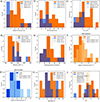 |
Fig. 3. Distributions of various ICME properties. Panel a: Distribution of the average duration of the sheath. Panel b: Average duration of MO. Panel c: Average magnitude of the magnetic field. Panel d: Average velocity inside the MO. Panel e: Percentage of disturbed part identified inside MO. Panel f: Velocity profile inside MO for HSS behind cases. Panel g: HSS in front cases. Panel h: Difference between the average velocity of MO and maximum velocity of HSS in percentage. Panel i: DiP. |
We find that, for HSS in front cases, 77% of the ICME events show no discernible sheath region before the start of the MO, while for HSS behind cases, only 20% of ICMEs are without a sheath region. This is expected as for HSS in front cases, the ICME is locally engulfed in the HSS, mostly having comparable plasma speeds upstream, which hinders the pileup of plasma and formation of a sheath region (e.g. Temmer et al. 2021). Interestingly, two of the HSS in front events reveal an ICME sheath duration of around ∼24 h, which is well above the average of 11 h as noted by Kilpua et al. (2017). Out of these, one ICME has a significantly higher velocity than the HSS; whereas for the other, the sheath is in the vicinity of the SIR compression region, making a clear distinction from the ICME sheath difficult.
Looking at the MO duration in panel b of Fig. 3, for cases of HSS behind, we derived a longer MO duration of 28.54 hours on average, compared to 18.8 hours for HSS in front cases. Both Mann-Whitney-U and Student’s t-tests suggest a statistically significant difference between the two distributions. We note that the MO duration is lower for HSS in front cases and higher for HSS behind cases when compared to typical ICMEs (i.e. approx. 24 hours according to Nieves-Chinchilla et al. 2018). The smaller duration of MO for HSS in front cases could point to significant flux rope erosion effects or different magnetic field draping behaviour in the scenario.
We find that the average magnetic field strength is lower for HSS in front cases (8.3 nT) compared to HSS behind cases (11.4 nT; see panel c, Fig. 3). Both statistical significance tests point to a significant difference in distributions. We note that in both cases. the average magnetic field is comparable to the total magnetic field of typical ICMEs (i.e. approx. 10 nT, according to Richardson & Cane 2010).
Next, we analysed the average speed of the MO (see panel d) in Fig. 3). We found a statistically significant difference between the distributions, with HSS in front cases having higher values (median 472 kms−1) compared to HSS behind (median 401 kms−1). This suggests that the HSS in front cases are where the ICME and HSS have comparable velocities. Although ICMEs could have speeds of 1000 kms−1, events in this upper limit are less prominent, with the average ICME having speeds of around 450 kms−1 (e.g. Richardson & Cane 2010). In contrast, HSSs tend to have speeds around 750–800 kms−1 (e.g. Richardson 2018). Hence, ICMEs travelling behind or catching up with the HSS should be less prevalent compared to HSS catching up with ICMEs. This is substantiated by our sample distribution too, since we only found 8 HSS in front cases, compared to 20 HSS behind cases, and we only found one case where the ICME was substantially faster than HSS. We note here that the average speed in both is comparable to average ICME speeds (Richardson & Cane 2010).
Next, we analysed the fraction of the disturbed part of the MO. The results are presented in panel e of Figure 3. We can see that in both cases, the distribution is slightly asymmetric. HSS in front cases show a larger proportion of undisturbed MOs tailing towards higher fractions. HSS behind cases show no specific trait, with the distribution revealing that the MOs are partially disturbed to some extent for most cases. Therefore, for most of the events, we expect to see only a fraction of MO disturbed. This is likely the reason why we do not derive a significant difference in the average MO properties compared to typical ICMEs. We also see that ICMEs with HSS behind tend to have somewhat higher fractions of the disturbed part of MO, compared to cases where the HSS is in front; however, the difference has not been confirmed by the statistical significance tests, possibly due to the small sample size. Nevertheless, this slight difference may indicate that an HSS catching up and compressing the ICME from the back disturbs it more easily than when the ICME is catching up with the HSS. A possible explanation could be that when HSS catches up with an ICME, a compressed and elevated magnetic field at the SI region readily acts as an obstacle for the ICME. On the other hand, when an ICME catches up with an HSS, there is no obstacle for the MO until it traverses the whole HSS and reaches the SI at the front.
We further inspected the speed profiles. For that, we first analysed the slopes of the speed profile within the MO, separately from the front and back regions. The average slopes calculated for the MO for either case are shown in panels f and g of Fig. 3. For undisturbed ICMEs, we expect a negative slope indicating a monotonically decreasing profile. We can see that the distributions of slopes in the front and back for HSS in front cases are shifted towards lower negative values, whereas for HSS behind cases show a distinct distribution of slopes. The front part shows a higher negative slope, while the back portion seems to be centred around zero (median 0.07 kms−2), although the spread is high. This difference in slope between the front and back parts is found to be statistically significant when the Student’s t-test is performed. This suggests that HSS in front cases tend to have more undisturbed-expanding speed profiles for the MO, whereas HSS behind cases can show a variety of scenarios for the MO expansion (monotonically decreasing profile, flat profile or accelerated profile). This is in agreement with the scenarios considered in Section 2.2. This result is also confirmed by performing a superposed epoch analysis (SEA), which is described in more detail in the following.
The SEA results, as shown in Fig. 4, clearly suggest an accelerated profile for HSS behind cases and a monotonically decreasing speed profile for HSS in front cases. We further confirm this result through visual inspection of speed profiles plotted in Appendix A (see Fig. A.1). We can see that for cases where the ICME is in front, 45% show partially disturbed profiles comparable to the scenario in Fig. 2b, while 25% show fully disturbed and accelerated profiles corresponding to the scenario in Fig. 2c. The remaining 30% show expansion traits. For the cases where the ICME is behind HSS, 62% show expansion traits with a largely undisturbed profile. Out of these, 10% corresponds to scenario Fig. 2d and 90% corresponds to scenario Fig. 2e. We note that the remaining 38% of ICMEs propagating behind HSS events do not adhere to scenarios proposed in Fig. 2 (three events showing bumpy and non-coherent speed profiles; see Appendix A).
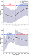 |
Fig. 4. Results from SEA. Top: Mean velocity and standard deviation from SEA for cases where the HSS is behind the ICME. Bottom: Same for cases where the HSS is in front of the ICME. |
We compared the relative difference in percentage between the average velocity and the HSS maximum speed. This is shown in panel h in Fig. 3. Since the solar wind tends to accelerate or decelerate the ICME to equalise the velocity difference (e.g. Vršnak et al. 2014), prolonged interactions should reflect a reduced velocity difference between the ICME and HSS in the distribution. Although the relative difference in velocities for HSS behind seems to have a higher median (22.5%) compared to HSS in front (12.5%), we find that the difference between the distributions is statistically insignificant. The large spread in the distribution might suggest that we are sampling a wide range of interaction durations since, presumably, during the interaction, there is a tendency to adjust the ICME speed to that of an HSS.
Next, we analysed the distortion of the MO using the DiP parameter, as described in Section 2.3. The results are shown in panel i of Fig. 3. We did not find a significant difference for either case, indicating there is no preferred enhancement to the magnetic field in the front or rear part of the MO in general. We note that we repeated the analysis for the so-called local DiP, which is defined on a subregion of MO (front, mid, and back), and obtained similar results (not shown here). We also note that the calculated DiP corresponds well to the median DiP of 0.47, as given by Nieves-Chinchilla et al. (2018). Looking at flux rope types as categorised in Nieves-Chinchilla et al. (2018), we find that 43% of the MOs in our sample represent the Fr type, 18% the Cx type, 18% the F− type, and the remaining 21% represent the F+ type. This is generally comparable to percentages obtained for a general ICME + MO sample (43%, 18%, 16%, and 14% for Fr, F−, F + , and Cx type, respectively, according to Nieves-Chinchilla et al. 2019), with a slightly more complex type of MOs and slightly more F+ type MOs.
Finally, we searched for reconnection exhausts and found ten events with reconnection exhausts observed at the front or back of the ICME. Among these, seven (three) were observed for HSS behind (in front) events. For HSS behind cases, all except one (found inside MO) reconnection exhausts were found at the back of the MO. The three reconnection exhausts found for HSS in front cases were found at the front of the MO. Thus, there is a clear tendency for the reconnection exhausts to appear at the interface between the magnetic obstacle of the ICME and the HSS.
We analysed the properties of reconnection exhausts and compared them to previous studies of general properties of reconnection exhausts in the solar wind. We first analysed the duration of the reconnection exhaust. We find that seven events (five in HSS behind cases and two in HSS in front cases) have a duration of less than three minutes (see the second last column of Table B.2). The remaining three display a longer duration, with a maximum of 40 minutes (2400 s). Among our results, one event shows unusually long temporal width compared to previous statistical studies (e.g. Mistry et al. 2017), where they found durations ranging from 3.7 s to 1610 s with a median of 42 s (see the fourth column of Table B.2). We find similar conclusions from analysing the width of reconnection exhausts (see the last column of Table B.2), which also compares well with a previous statistical study done in solar wind (Mistry et al. 2017) except for one event showing unusually long duration of 40 minutes. We then calculated the averages of reconnection parameters for HSS in front (HSS behind) case according to Equations (3) through (7):
-
θ−121(°);
-
Brec−6.3(11.3) nT;
-
Vacc−10(23) km−1;
-
Nenh−1.4(0.9) cm−3;
-
Tenh−1.6(3.2) eV.
The calculated averages of reconnection parameters are fully comparable to the results from the parameters as calculated in Enžl et al. (2014). Therefore, the reconnection exhausts do not seem to reveal any difference in the ICME-HSS interactions compared to solar wind in general.
4. Summary and conclusion
We analysed in situ signatures of 28 ICMEs interacting with HSSs at 1 AU between 2010 and 20183 to identify and characterise their common interaction features. In particular, we analysed the ICME velocity profiles, duration of the sheath and MO, and distortion of the MO. In addition, we searched for the signatures of reconnection exhausts. We found 20 events where the HSS is behind the ICMEs and 8 events where the HSS is in front of the ICME. Atatistical analysis was performed for these two classes of interaction separately. Our general findings are given below.
-
The sheath formation is clearly inhibited when the HSS is in front of the ICME, with ∼70% of the cases showing no discernible sheath region.
-
The MO duration is shorter for HSS in front cases compared to the HSS behind cases.
-
The average magnetic field amplitude is larger for HSS behind cases compared to HSS in front.
-
The average speed of ICMEs tends to be lower for HSS behind cases compared to HSS in front cases. This is expected since the HSSs in general are faster than the average ICMEs, while the ICMEs having speeds of the order of HSSs are less prevalent. This is also reflected in our sample size of 20 for HSS behind and 8 for HSS in front.
-
The MO speed profile may be significantly different from the expected speed profile of undisturbed MO, its shape depending on whether the HSS is in front or behind. In particular, we find that the velocity profile of HSS in front events generally shows an expanding profile, while the HSS behind show a compressed profile toward the rear of the MO.
-
The magnetic field of MO does not show preferential amplification towards the front or rear portion of the MO.
-
Reconnection exhaust signatures are found in 35% of ICME-HSS interactions, dominantly at the interface of ICME and HSS. The observed reconnection exhaust properties are similar to those of the reconnection exhaust in general.
-
Comparing the average percentage of disturbed part of MO and the difference between the average velocities of HSS and ICMEs shows no statistically significant difference. Since the prolonged interaction tends to equalise the velocity of ICME to that of HSS (to a first approximation), the latter suggests that we are sampling from a large number of interaction scenarios.
Although the average values of MO duration, average magnetic field strength, and average velocity are comparable to those reported in existing literature, statistical significance tests reveal meaningful differences in their distributions. Specifically, when analysing separately the interaction scenarios where an HSS is located either behind or in front of an ICME, statistically significant variations emerge. These differences highlight the impact of HSS-ICME interactions on the physical properties of the ICME.
To summarise, we find that ICMEs interacting with HSS in general do not show distinctly different properties compared to typical ICMEs; however, they do show distinct differences when resolved into cases where HSS is behind the ICME and HSS is in front of the ICME. We find that the HSS in front cases tend to inhibit the formation of the sheath and shows a lower average magnetic field magnitude inside the MO. This could point to erosion effects and/or different draping behaviour of magnetic field lines, which would be an interesting topic for further investigation. We also find that HSSs catching up to ICMEs tend to compress them from the back, whereas HSSs in front of ICMEs do not significantly alter the typical speed expansion profiles. Although we find reconnection exhaust signatures in about 35% of events, we do not find significant evidence of the distortion of the internal magnetic structure. Our results indicate that an interaction with an HSS does not significantly influence an ICME’s internal magnetic structure; however, it could significantly influence its kinematics.
Acknowledgments
We acknowledge the support by the Croatian Science Foundation under the project IP-2020-02-9893 (ICOHOSS), the European Union – NextGenerationEU within the framework of the National Recovery and Resilience Plan (NPOO), project “Eruptive processes on the Sun”, and from the Austrian-Croatian Bilateral Scientific Project “Analysis of solar eruptive phenomena from cradle to grave”. A.K.R. acknowledges support from the Croatian Science Foundation in the scope of the Young Researchers Career Development Project Training New Doctoral Students. The work of N.F. is funded by the CNES (Centre National d’Etudes Spatiales) and CNRS (Centre national de la Recherche Scientifique). We thank the science teams of ACE, and Wind for providing the data and maintaining the spacecraft.
References
- Acuña, M. H., Ogilvie, K. W., Baker, D. N., et al. 1995, Space Sci. Rev., 71, 5 [Google Scholar]
- Burlaga, L., Sittler, E., Mariani, F., & Schwenn, R. 1981, J. Geophys. Res., 86, 6673 [Google Scholar]
- Chree, C. 1913, Proc. Phys. Soc. London, 26, 137 [Google Scholar]
- Dasso, S., Nakwacki, M. S., Démoulin, P., & Mandrini, C. H. 2007, Sol. Phys., 244, 115 [Google Scholar]
- Dumbović, M., Guo, J., Temmer, M., et al. 2019, ApJ, 880, 18 [Google Scholar]
- Dumbović, M., Vršnak, B., Temmer, M., Heber, B., & Kühl, P. 2022, A&A, 658, 187 [Google Scholar]
- Enžl, J., Přech, L., Šafránková, J., & Němeček, Z. 2014, ApJ, 796, 21 [CrossRef] [Google Scholar]
- Gosling, J. T., & Phan, T. D. 2013, ApJ, 763, L39 [Google Scholar]
- Gulisano, A. M., Démoulin, P., Dasso, S., Ruiz, M. E., & Marsch, E. 2010, A&A, 509, A39 [NASA ADS] [CrossRef] [EDP Sciences] [Google Scholar]
- He, W., Liu, Y. D., Hu, H., Wang, R., & Zhao, X. 2018, ApJ, 860, 78 [NASA ADS] [CrossRef] [Google Scholar]
- Heinemann, S. G., Temmer, M., Farrugia, C. J., et al. 2019a, Sol. Phys., 294, 121 [NASA ADS] [CrossRef] [Google Scholar]
- Heinemann, S. G., Temmer, M., Heinemann, N., et al. 2019b, Sol. Phys., 294, 144 [NASA ADS] [CrossRef] [Google Scholar]
- Heinemann, S. G., Sishtla, C., Good, S., Grandin, M., & Pomoell, J. 2024, ApJ, 963, L25 [Google Scholar]
- Hudson, P. 1970, Planet. Space Sci., 18, 1611 [Google Scholar]
- Karuppiah, S., Dumbović, M., Martinić, K., et al. 2024, Sol. Phys., 299, 87 [Google Scholar]
- Kay, C., Nieves-Chinchilla, T., Hofmeister, S. J., & Palmerio, E. 2022, Space Weather, 20, e2022SW003165 [NASA ADS] [Google Scholar]
- Kilpua, E., Koskinen, H. E. J., & Pulkkinen, T. I. 2017, Liv. Rev. Sol. Phys., 14, 5 [Google Scholar]
- King, J. H., & Papitashvili, N. E. 2020, OMNI 5-min Data Set [Google Scholar]
- Lopez, R. E. 1987, J. Geophys. Res., 92, 11189 [Google Scholar]
- Mann, H. B., & Whitney, D. R. 1947, Ann. Math. Stat., 18, 50 [Google Scholar]
- Mistry, R., Eastwood, J. P., Phan, T. D., & Hietala, H. 2017, J. Geophys. Res.: Space Phys., 122, 5895 [NASA ADS] [CrossRef] [Google Scholar]
- Nieves-Chinchilla, T., Vourlidas, A., Raymond, J. C., et al. 2018, Sol. Phys., 293, 25 [NASA ADS] [CrossRef] [Google Scholar]
- Nieves-Chinchilla, T., Jian, L. K., Balmaceda, L., et al. 2019, Sol. Phys., 294, 89 [Google Scholar]
- Pal, S., Kilpua, E., Good, S., Pomoell, J., & Price, D. J. 2021, A&A, 650, A176 [NASA ADS] [CrossRef] [EDP Sciences] [Google Scholar]
- Richardson, I. G. 2006, in Recurrent Magnetic Storms: Corotating Solar Wind, eds. R. McPherron, W. Gonzalez, G. Lu, H. A. José, & S. Natchimuthukonar Gopalswamy, 167, 45 [Google Scholar]
- Richardson, I. G. 2018, Liv. Rev. Sol. Phys., 15, 1 [Google Scholar]
- Richardson, I. G., & Cane, H. V. 2010, Sol. Phys., 264, 189 [NASA ADS] [CrossRef] [Google Scholar]
- Ruffenach, A., Lavraud, B., Farrugia, C. J., et al. 2015, J. Geophys. Res.: Space Phys., 120, 43 [Google Scholar]
- Scolini, C., Winslow, R. M., Lugaz, N., et al. 2022, ApJ, 927, 102 [NASA ADS] [CrossRef] [Google Scholar]
- Stone, E. C., Frandsen, A. M., Mewaldt, R. A., et al. 1998, Space Sci. Rev., 86, 1 [Google Scholar]
- STUDENT 1908, Biometrika, 6, 1 [CrossRef] [Google Scholar]
- Temmer, M. 2021, Liv. Rev. Sol. Phys., 18, 4 [NASA ADS] [CrossRef] [Google Scholar]
- Temmer, M., Holzknecht, L., Dumbović, M., et al. 2021, J. Geophys. Res.: Space Phys., 126, e28380 [NASA ADS] [CrossRef] [Google Scholar]
- Tilquin, H., Eastwood, J. P., & Phan, T. D. 2020, ApJ, 895, 68 [NASA ADS] [CrossRef] [Google Scholar]
- Vršnak, B., Temmer, M., Žic, T., et al. 2014, ApJS, 213, 21 [CrossRef] [Google Scholar]
- Winslow, R. M., Lugaz, N., Schwadron, N. A., et al. 2016, J. Geophys. Res.: Space Phys., 121, 6092 [Google Scholar]
- Winslow, R. M., Scolini, C., Lugaz, N., & Galvin, A. B. 2021, ApJ, 916, 40 [NASA ADS] [CrossRef] [Google Scholar]
- Xu, F., & Borovsky, J. E. 2015, J. Geophys. Res.: Space Phys., 120, 70 [NASA ADS] [CrossRef] [Google Scholar]
Appendix A: Ancillary figures
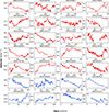 |
Fig. A.1. Velocity profiles inside MO. Plots in red show the cases where the HSS is behind the ICME, and plots in blue show the cases where the HSS is in front of the ICME. |
Appendix B: Tables
List of events
List of reconnection exhausts
All Tables
All Figures
|
Fig. 1. Plots showing examples of ICME-HSS interaction and HSS-ICME interaction. Top panel: Magnetic field components in GSE coordinates. Second panel: Proton temperature (black) over plotted with the expected plasma temperature (red) and plasma density (blue). Third panel: Plasma velocity. Fourth panel: Plasma beta. Fifth panel: Plasma entropy (grey) and azimuthal (longitudinal) plasma flow angle (red). The horizontal red line in panel four marks the value one for plasma beta, the horizontal red line in panel four marks the value four for plasma entropy, while the horizontal black line marks zero for azimuthal flow angle. The shaded grey regions show the HSS (from the stream interface to the end), whereas the vertical black lines mark the start and end of the MO. The shaded brown region in the left panels marks the disturbed region (the zoomed-in plot highlights the same with the front and back of the MO marked with red and blue arrows, respectively. For more details, see the main text). The shaded purple region in the right panels marks the compression region + SIR. |
| In the text | |
|
Fig. 2. Sketch showing different hypothesised speed profiles inside MO: a) undisturbed MO; b) slower CME is accelerated by the faster HSS behind for a shorter time period; c) lower CME is accelerated by the faster HSS behind for a longer time period; d) CME faster than the HSS is catching up with it; e) CME moving with the HSS. For details, see the main text. |
| In the text | |
|
Fig. 3. Distributions of various ICME properties. Panel a: Distribution of the average duration of the sheath. Panel b: Average duration of MO. Panel c: Average magnitude of the magnetic field. Panel d: Average velocity inside the MO. Panel e: Percentage of disturbed part identified inside MO. Panel f: Velocity profile inside MO for HSS behind cases. Panel g: HSS in front cases. Panel h: Difference between the average velocity of MO and maximum velocity of HSS in percentage. Panel i: DiP. |
| In the text | |
|
Fig. 4. Results from SEA. Top: Mean velocity and standard deviation from SEA for cases where the HSS is behind the ICME. Bottom: Same for cases where the HSS is in front of the ICME. |
| In the text | |
|
Fig. A.1. Velocity profiles inside MO. Plots in red show the cases where the HSS is behind the ICME, and plots in blue show the cases where the HSS is in front of the ICME. |
| In the text | |
Current usage metrics show cumulative count of Article Views (full-text article views including HTML views, PDF and ePub downloads, according to the available data) and Abstracts Views on Vision4Press platform.
Data correspond to usage on the plateform after 2015. The current usage metrics is available 48-96 hours after online publication and is updated daily on week days.
Initial download of the metrics may take a while.