| Issue |
A&A
Volume 707, March 2026
|
|
|---|---|---|
| Article Number | A79 | |
| Number of page(s) | 8 | |
| Section | Interstellar and circumstellar matter | |
| DOI | https://doi.org/10.1051/0004-6361/202555808 | |
| Published online | 09 March 2026 | |
The gas streamer G1–2–3 in the Galactic center
1
Max Planck Institute for extraterrestrial Physics,
Giessenbachstraße 1,
85748
Garching,
Germany
2
Departments of Physics and Astronomy, Le Conte Hall, University of California,
Berkeley,
CA
94720,
USA
3
Technical University of Munich,
85747
Garching,
Germany
4
Universidad Adolfo Ibañez,
Av. Padre Hurtado 750,
Viña del Mar,
Chile
5
Max Planck Institute for Astrophysics,
Karl-Schwarzschild-Straße 1,
85748
Garching,
Germany
6
University Observatory Munich,
Scheinerstraße 1,
81679
Munich,
Germany
7
Racah Institute for Physics, The Hebrew University,
Jerusalem
91904,
Israel
8
Department of Physics and Astronomy, Bartol Research Institute, University of Delaware,
Newark,
DE
19716,
USA
9
Millennium Nucleus on Transversal Research and Technology to Explore Supermassive Black Holes (TITANS),
Chile
10
INAF – Osservatorio Astrofisico di Arcetri,
Largo E. Fermi 5.,
50125,
Firenze,
Italy
11
INAF – Osservatorio Astronomico d’Abruzzo,
Via Mentore Maggini,
64100
Teramo,
Italy
12
INAF – Osservatorio Astronomico di Padova,
Vicolo dell’Osservatorio 5,
35122
Padova,
Italy
13
STFC UK ATC, Royal Observatory Edinburgh,
Blackford Hill. Edinburgh
EH9 3HJ,
UK
14
ETH Zurich, Institute of Particle Physics and Astrophysics,
Wolfgang-Pauli-Strasse 27,
8093
Zurich,
Switzerland
15
Leiden Observatory, University of Leiden,
PO Box 9513,
2300 RA
Leiden,
The Netherlands
16
I. Physikalisches Institut, Universität zu Köln,
Zülpicher Str. 77,
50937
Köln,
Germany
★ Corresponding author: This email address is being protected from spambots. You need JavaScript enabled to view it.
Received:
4
June
2025
Accepted:
16
January
2026
Abstract
The black hole in the Galactic center, Sgr A*, is prototypical of ultra-low-fed galactic nuclei. The discovery of a handful of gas clumps with masses on the order of a few Earth masses in its immediate vicinity provides a gas reservoir sufficient to power Sgr A*. In particular, the gas cloud G2 is of interest due to its extreme orbit, on which it passed at a pericenter distance of around 100 AU and notably lost kinetic energy during the fly-by due to interaction with the black hole accretion flow. Thirteen years prior to G2, a similar gas cloud called G1, passed Sgr A* on a similar orbit. The origin of G2 remained a topic of discussion, with models including a central (stellar) source still proposed as alternatives to pure gas clouds. Here, we report the orbit of a third gas clump moving along (nearly) the same orbital trace. Since the probability of finding three stars on such similar orbits is very low, this strongly argues against stellar-based source models. Instead, we show that the gas streamer G1–2–3 plausibly originates from the stellar wind of the massive binary star IRS 16SW. This claim is substantiated by the fact that the small differences between the three orbits – the orientations of the orbital ellipses in their common plane as a function of time – are consistent with the orbital motion of IRS 16SW.
Key words: black hole physics / gravitation / celestial mechanics / binaries: close / ISM: clouds / Galaxy: center
© The Authors 2026
 Open Access article, published by EDP Sciences, under the terms of the Creative Commons Attribution License (https://creativecommons.org/licenses/by/4.0), which permits unrestricted use, distribution, and reproduction in any medium, provided the original work is properly cited.
This article is published in open access under the Subscribe to Open model.
Open Access funding provided by Max Planck Society.
1 Introduction
The peculiar object G2 in the Galactic center was identified in Gillessen et al. (2012) as an object apparently residing between the S-stars (Eckart & Genzel 1996; Ghez et al. 1998; Schödel et al. 2002; Ghez et al. 2003; Eisenhauer et al. 2005; Ghez et al. 2008; Gillessen et al. 2009; Gillessen et al. 2017; Gravity Collaboration 2024). G2 showed the properties of a dusty, ionized gas cloud, with line emission from hydrogen and helium, and thermal emission corresponding to 600 K. No emission from a potential stellar photosphere (T ≳ 3000 K) was convincingly detected, as the claimed K-band detection in Eckart et al. (2013) remained episodic. G2 was spatially marginally resolved (at the ∼60 mas resolution of the 8m VLT in the K band) and – more importantly – spectrally showed a velocity gradient across the source.
Multiyear adaptive optics imaging (with NACO; see Lenzen et al. 1998; Rousset et al. 1998) and integral field spectroscopy (with SINFONI; see Eisenhauer et al. 2003; Bonnet et al. 2003) in the near-infrared showed that G2 was approaching Sgr A* on a highly eccentric orbit with pericenter passage in 2014 (Witzel et al. 2014; Gillessen et al. 2013). Position-velocity diagrams from subsequent years showed spectacular tidal evolution of the gas stretching along the orbital trace (Pfuhl et al. 2015; Plewa et al. 2017).
Given its measured size of around 120 AU, thermal luminosity, and temperature, it is clear that G2 is optically thin and fully ionized by the UV photons from the surrounding young, massive stars. From the Brackett-γ luminosity and assuming case B recombination theory, the gas mass of G2 was estimated to be ≲3 Earth masses.
With the gas of G2 nearly radially infalling, a number of papers addressed whether a radiative reaction would be observable around pericenter passage (Gillessen et al. 2012; Narayan et al. 2012; Crumley & Kumar 2013; Bartos et al. 2013). The absence of any such events does not, however, yield strong constraints on possible source models. Ponti et al. (2015) report a mildly increased rate of X-ray flares from Sgr A* following G2’s post-pericenter passage.
Pfuhl et al. (2015) noted that 12 years ahead of G2, a very similar – although somewhat fainter – object was moving along a very similar trajectory, which they called G1. The dust emission of this object was also noted already in very early adaptive-optics images (Clénet et al. 2005), where it appeared spatially extended (Ghez et al. 2005) and also showed tidal evolution along the orbit (Witzel et al. 2017). Further, a tail follows behind G2 on apparently a similar orbit. One could thus think of G1, G2, and the tail as knots in a long gas streamer, of which we detect only the brightest peaks in sensitivity-limited observations, aided by the fact that the observed surface brightness of the gas scales as density squared.
The long gas streamer is actually visible in deep spectroscopic integrations (see figures 9 and 10 in Plewa et al. 2017). It points spatially and in radial velocity back to the stellar wind of the contact binary system IRS 16SW (Ott et al. 1999; Martins et al. 2006). That star is classified as Ofpe/WN9 and is a member of the clockwise (CW) disk of young stars (Levin & Beloborodov 2003; Paumard et al. 2006; Lu et al. 2009; Bartko et al. 2009; Yelda et al. 2014; von Fellenberg et al. 2022; Jia et al. 2023); G2 and G1 orbit Sgr A* in that same plane. In hydrodynamical simulations (Cuadra et al. 2006; Calderón et al. 2020b) the star significantly contributes to the gas found around Sgr A*, and its spectrum observationally shows signs of strong winds.
The post-pericenter motion of G2 is actually better described by adding a ram-pressure-like drag force to the Keplerian model (Pfuhl et al. 2015; McCourt & Madigan 2016; Madigan et al. 2017; Gillessen et al. 2019). G2 decelerates due the interaction with the accretion flow of Sgr A*(Yuan et al. 2003; Yuan & Narayan 2014), the density of which follows roughly a radial profile ∝ r−1. G2’s motion thus provides a valuable measurement of the accretion flow density at around 103 Schwarzschild radii rS , which otherwise is constrained mostly around 10 rS from sub-millimeter observations (Agol 2000; Quataert & Gruzinov 2000; Bower et al. 2003; Marrone et al. 2006, 2007; Bower et al. 2015) or around 105 rS from X-ray observations (Baganoff et al. 2003; Wang et al. 2013).
Given the strong evidence for gaseous, tidal evolution in G2, it is clear that the observed gas cannot be gravitationally bound to a central source. With the measured size of G2 (≈20 mas) around the time of detection (Gillessen et al. 2012), the mass required to bind gas on that scale would exceed 104 M⊙ – i.e., an intermediate mass black hole – which is excluded at such small radii (Gillessen et al. 2009; Naoz et al. 2020; Reid & Brunthaler 2020; Gravity Collaboration 2023). Yet, this does not exclude the possibility of a central stellar source as the gas origin.
Observationally, there is no need to invoke a central object for G2. All its properties can be explained without. It only has an L-band counterpart but is invisible in the K band. Also, the post-pericenter presence and appearance of G2 are not strong discriminators, as purely gaseous models do not predict complete disruption of the cloud; see for example Fig. 2 in Schartmann et al. (2015). Still, models with a central source have been discussed and often favored (Phifer et al. 2013; Witzel et al. 2014). Scoville & Burkert (2013) proposed a young low-mass star, whose wind would create G2. Meyer & Meyer-Hofmeister (2012) discussed a stellar nova as the origin for G2. Tidal interactions of a star with Sgr A* have also been proposed, either from a disk around the star (Murray-Clay & Loeb 2012; Miralda-Escudé 2012) or a true partial tidal disruption of a giant star (Guillochon et al. 2014).
Perhaps the most extreme proposal is that not only G2, but also other similar gas knots (Ciurlo et al. 2020), are binary merger products (Witzel et al. 2014), driven by the Kozai-Lidov mechanism (Prodan et al. 2015; Stephan et al. 2016). This picture requires a number of assumptions – from the presence and merger of binaries close to Sgr A* to how such an object would appear, how long they would remain visible, and how likely it would be to observe several simultaneously – given that the total number of stars exceeds the number of mergers from which they arise by a factor of 20.
Here, we present new observational evidence supporting the gas streamer picture: the emission that formed the outer tail “G2t” at the time of G2’s discovery has now evolved into a clump resembling G2 in 2008 – thus constituting a third object moving along nearly the same trajectory. Given the properties of G1, G2, and the new clump, it is natural to consider them together as a gas streamer, which we call G1–2–31.
2 Observations
Our data are based on adaptive-optics-assisted integral field spectroscopy: pre-2020 with SINFONI, and since 2022 with ERIS (Davies et al. 2023). Both instruments use the same integral field unit (IFU). We employed the 25 mas pixel scale and observed the K band, concentrating the analysis on the Brackett-γ emission (vacuum rest wavelength 2.16612 µm). Since these data also serve to monitor the radial velocities of the S-stars, we covered a field of view of around ±0.6″ by dithering the 0.8″ field-of-view IFU into four quadrants offset by ±0.2″ from Sgr A* in both coordinates. G2t is located around (∆α, ∆δ) = (+0.3, −0.1)″ from Sgr A*, comfortably within the data cubes.
The top row in Figure 1 illustrates the ERIS data cube from June / July 2024.
The exposure time is 600 s per data cube. Given the faintness of the line emission from G1–2–3, we combined the data from one observing campaign lasting a few nights into a combined cube in order to reach fainter magnitudes. Prior to combining, we aligned the cubes in all three dimensions, neglecting the small change in the local standard of rest (LSR). Table A.1 in the appendix summarizes the data used for G2t.
3 Analysis
3.1 The orbits of G1, G2, and G2t
Using QFitsView (Ott, T. 2025), we identified the G2t emission around Brackett-γ. For obtaining an estimate of G2t’s orbit, we measured the position and radial velocity of the emission line. Since it is extended both spatially and spectrally, this was done manually to capture the major part of the emission around its peak. The bottom row of Figure 1 shows an example of the data cube from June/July 2024. The spectral and spatial line positions were obtained via simple Gaussian fits. Using the pixel scale of 12.5 mas/pix, positions were referenced to Sgr A* via S2, whose orbit is known to much higher precision than required for G2t. For the radial velocities we applied the standard LSR correction. Due to its extended nature, we assigned conservative error bars of 10 mas spatially (at least) and 50 km/s spectrally. We obtained positions from six epochs, and radial velocities from eight epochs between 2014 and 2025 in this way. For G2, compared to Gillessen et al. (2019), we obtained five more ERIS-based radial velocities and four more positions in the same way, yielding a total of 23 velocities and 18 positions.
At this point, G2t’s astrometry shows no significant acceleration toward Sgr A*, but a >9σ significant change in radial velocity is observed, providing enough dynamic quantities to determine an orbit (with six degrees of freedom) in a fixed gravitational potential. The data are shown in Figure 2. A preliminary orbit fit for G2t (Table B.1) shows that its orbital plane, orientation, shape, and size are similar to those of G2 (and thus also close to the CW disk and G1; Pfuhl et al. 2015). Finding three objects by chance on such similar orbits is very unlikely. The probability that two orbital planes agree to within ±θ is p1 = 2π(1 − cos θ)/4π. The probability that the orientations of the ellipses in the plane agree to within ±θ is p2 = θ/π. The probability of finding three such orbits by chance is therefore  , which evaluates to p = 2 × 10⁻⁶ for θ = 15°. Similarity in orbital phase, eccentricity, and semimajor axis further reduces p. Hence, one can exclude a random alignment.
This is the motivation for our proposed model: the three clumps share (almost) identical orbits due to their common origin from IRS 16SW. We therefore fit the three orbits under strong side constraints: they must be coplanar and share a common semimajor axis and eccentricity. The only allowed differences are the times of pericenter passage and the longitudes of periastron, which correspond to the orientation of the orbital ellipses within their common plane. The gravitational potential is taken from GRAVITY Collaboration (2022) and kept fixed (this is: M = 4.296 × 10⁶ M⊙, R0 = 8.275 kpc, and the coordinate system parameters for the central mass). The drag force model is used (and fit) as in Gillessen et al. (2019) for all three orbits. The resulting model (see Table B.2) is shown overlaid on the data in Figure 2. It is a very good description of the data, which is a very remarkable finding. Fitting the G2, G1, and G2t individually, with each fit having six free parameters (and an additional drag force parameter for G2), yields χ2 values of 115.6, 36.5, and 26.4 for 50, 14, and 14 degrees of freedom, respectively. This gives a total χ2 of 178.5. The combined fit is only slightly worse, with χ2 = 196.6, despite having eight fewer free parameters. For another representation of the combined fit, see Figure C.1 and Appendix B for the orbital elements.
The apocenter distance of the orbits is around 1.9″ and occurred around the mid of the 19th century. The apocenters are not far from the position of IRS 16SW at that time (using the orbit from Gillessen et al. 2017). An exact agreement is not expected, as the gas clumps originate from the winds of IRS 16SW (or from shocks created by them), which themselves have significant velocities of a few hundred kilometers per second. Also the orbital planes do not agree perfectly but differ by ≲30°, which likely reflects the fact that the initial conditions of the gas clouds do not need to coincide exactly with those of the star. When fit individually, G2 attains a larger apocenter distance and G2t a smaller one. This may indeed be more realistic, as individual clumps arising in the stellar wind can have different initial conditions. In that view, the orbital planes can also differ a bit between the three clumps and the star. Also, previous work found that the best-fitting orbits of G1 and G2 do not completely agree (Pfuhl et al. 2015; Witzel et al. 2017). Nevertheless, the point of the combined fit employed here is that the model – in which G1 and G2t only have two free parameters each (pericenter time and longitude of pericenter) – describes the data remarkably well.
Using the combined fit, G2t’s pericenter passage will occur 17.6 ± 0.3 yr after that of G2, i.e., in mid 2031. The pericenter longitudes differ by 12.9 ± 1.1° between G2 and G2t, with the G2t orbit rotated CW relative to the G2 orbit. These two numbers correspond to an angular speed of 0.74 ± 0.07°/yr. For G1, in comparison with G2, the same analysis yields an angular speed of 0.74 ± 0.10°/yr in the same direction (consistent with the value implied in Pfuhl et al. (2015) of 0.95 ± 0.63°/yr). Note that the numbers happen to be very close to each other; this was not a constraint for the fit. Furthermore, the value is remarkably close to the angular speed of IRS 16SW, which is around 1.11 ± 0.32°/yr at its orbital position around the year 1950. Thus, the differences between the G1, G2, and G2t orbits can be explained by the orbital motion of IRS 16SW. This further indicates that the star is the origin of the gas clouds. We note that other (CW-disk) stars in the vicinity could, in principle, also be responsible for the production of the gas clumps. Here we limit ourselves to discussing IRS 16SW, which we consider the most likely candidate.
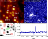 |
Fig. 1 G2t in the ERIS integral-field data from June/July 2024. Top left: continuum image showing the S-stars. Top right: Background-subtracted line map centered at 2.173 µm, corresponding to Brackett-γ + 1000 km/s. G2t stands out. Bottom left: example of a pixel selection (on – green, off – red) for extracting the G2t spectrum overlaid on the continuum map. Bottom right: Resulting spectrum showing a strong emission line at 2.173 µm. |
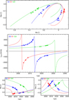 |
Fig. 2 Orbits and data of G1, G2, and G2t, fit under the constraint that they share the same orbital plane, semimajor axis, and eccentricity. Top: on-sky appearance of the two orbits. Middle: radial velocities. Bottom: spatial coordinates as a function of time. The non-Keplerian shapes result from the drag force acting on G2 and G2t when they are close to Sgr A*. |
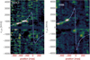 |
Fig. 3 Left: position–velocity diagram extracted from the June/July-2024 data cube, using a curved slit along the orbital trace of G2t. The emission of G2t is concentrated around (−300 mas, +1000km/s). Similar to G2, G2t seems to be followed by a tail, indicative of even more material flowing along the G1–2–3 path. Right: same diagram for G2 extracted from the 2008 data cube (from Gillessen et al. 2019) for comparison. |
3.2 Position-velocity diagram for G2t
Using the same technique as in Gillessen et al. (2019) for extracting a position-velocity diagram along the curved trajectory given by the orbit, we obtain the diagram shown in Figure 3. The G2t emission highly resembles G2 a few years before the latter’s pericenter passage. Notably, G2t also shows trailing emission, as G2 did and as mentioned in the discovery paper Gillessen et al. (2012), perhaps indicating a fourth clump forming within the next decade. The Brackett-γ luminosity of G2t is comparable to that of G2, though roughly 38% lower.
4 Discussion
With the ample hints linking G1–2–3 to IRS 16SW, it is worth reconsidering the formation of gas clumps from the winds of that source. This requires producing clouds with masses on the order of a few Earth masses at intervals of 10–20 years, yielding a time-averaged mass rate of ∼10−7 M⊙ yr−1. This constitutes a non-negligible fraction of around 1% of the Wolf-Rayet wind rate of ∼10−4.7 M⊙ yr−1 (Martins et al. 2007). Channeling such a substantial fraction of an initially quasi-spherical outflow toward the central black hole poses a significant dynamical challenge, as the gas must lose most of its orbital angular momentum. An anisotropic mass-loading geometry – possibly governed by the orientation of the IRS 16SW binary axis relative to its orbital motion – may be required to facilitate such an efficient mass transfer. Unfortunately, the orientation of the orbit is unknown, except that the system appears nearly edge-on, since it is observed as an eclipsing binary (Martins et al. 2006).
An alternative is to consider stellar wind interactions, both among themselves and with the surrounding medium. In each case, the stellar wind shocks create a dense slab, which, depending on its radiative properties, can be prone to cooling and hydrodynamic instabilities that result into the formation of clumps (Vishniac 1994). This process has been studied analytically and numerically for stellar wind collisions in binaries and random stellar encounters (Calderón et al. 2016, 2020a). These studies found that, for Galactic center stars, the clumps formed are smaller and lighter than those observed. Additionally, Calderón et al. (2018) investigated the hypothesis of binaries – specifically focusing on IRS 16SW – launching clumps into the medium and following their ballistic orbits. The results showed that it was not possible to reproduce the position and velocity of G2 if it formed from the binary. Thus, it would seem that IRS 16SW cannot be the source of the observed G1–2–3 clumps.
However, the simulations of Calderón et al. (2020b, 2025) of the entire Wolf-Rayet population in the Galactic center revealed a different clump formation mechanism that actually relies on the hydrodynamic interaction with the surrounding medium. This requires a relatively dense medium of ∼100 particles cm−3, as measured at the radial distance of IRS 16SW (Baganoff et al. 2003), and a stellar wind with a low terminal velocity of around 450 km s−1. The bow shock formed in this situation becomes unstable and breaks into clumps. Moreover, interaction with the medium slows the dense material and preferentially directs it into radial orbits toward Sgr A*, rendering the previous ballistic assumption invalid.
Previous models of Galactic center hydrodynamics (e.g. Cuadra et al. 2008, 2015; Ressler et al. 2018; Calderón et al. 2025) adopted 600 km s−1 for the stellar wind of IRS 16SW, based on its spectral features (Martins et al. 2007; Cuadra et al. 2008). While relatively low, this velocity did not produce an unstable bow shock in the models. IRS 16SW, however, is a contact binary (DePoy et al. 2004), so its outflow velocity can substantially differ from that determined from its atmospheric properties. High-resolution simulations of wind collisions in static stellar pairs by Calderón et al. (2020a) found that clumps formed by a symmetric binary are ejected at ≈3/5 of the individual stellar wind velocity, 360 km s−1 in this case. Although the orbit of the binary was not included in that model, we expect its internal velocity (also around 360 km s−1) can be added to or subtracted from the outflowing material, resulting in a range of effective outflow velocities from 0 to ≈700 km s−1. These low velocities could result in unstable bow shocks as described above.
To test this idea, we ran a simulation of the Wolf–Rayet stellar winds feeding Sgr A* using the setup of the control model (without feedback from Sgr A*) of Cuadra et al. (2015). In summary, we placed a system of 30 mass-losing stars on their observed orbits (Cuadra et al. 2008; Gillessen et al. 2017) with their constrained stellar wind properties (Martins et al. 2007; Cuadra et al. 2008), and evolved it for 1100 yr, starting in the past in order to recover the state of the system at the present time. Unlike our previous work, we used the state-of-the-art smoothed-particle hydrodynamic (SPH) code Phantom (Price et al. 2018, Russell et al. in prep.) to avoid the formation of spurious clumps in the generic SPH technique (e.g. Hobbs et al. 2013). While IRS 16SW should ideally be modeled as a binary, its compactness makes that impossible with our current setup. We therefore explored the effect of its expected slower wind by modeling it as a single source with wind speeds of 300 km s−1, 400 km s−1, and 600 km s−1. In all models the mass-loss rate of the source was kept at its original value of 1.12 × 10⁻⁵ M⊙ yr−1. The simulations with 300 km s−1 and 400 km s−1 do produce a dense bow shock around this source that fragments into several clumps and filaments, some of which enter orbits toward Sgr A* (see Figure 4), while remaining roughly in the same orbital plane as the source. The clumps produced in these simulations also have masses of the same order of magnitude as the observed ones. While there is some uncertainty in how clumps are defined, our simulation with a 300 km s−1 wind roughly produced 20 clumps in the inner arc second at the present time with masses above 3 Earth masses (see Figure D.1). This is, in principle, more than enough to explain the observed clumps. In a follow-up study, we will ascertain the robustness of this result to the numerical resolution and method (particle- or grid-based). These masses are much higher than those found in previous idealized stellar wind collision models (< 0.01 Earth masses; Calderón et al. 2018, 2020a), but their creation mechanism is very different. In the currently proposed scenario, the clumps form at the bow shock in front of IRS 16SW due to the wind-medium interaction, rather than from the wind-wind interaction within the binary system. Therefore, it seems possible that G1–2–3 originates from IRS 16SW, although the exact formation mechanism requires more detailed study that properly accounts for the binary nature of the source.
Finally, it is worth noting that accreting a single G2-like clump (with a mass ≈1 Earth mass) per decade suffices to explain the inferred accretion rate of ≈10−7.6 M⊙ yr−1 onto Sgr A* at the apocenter distance of G2 of ≈1000 RS (Yuan & Narayan 2014; Gillessen et al. 2019). Thus, the G1–2–3 streamer – decelerated by the drag force – could be the main current source of gas for Sgr A*, if the gas ≈50 yr after the first pericenter settles into the accretion flow. This notion is in agreement with the generally accepted view that Sgr A* is mostly fed directly by the hot plasma created by the stellar winds (Quataert et al. 1999; Cuadra et al. 2006). But it is more specific. Clump formation occurs preferentially when IRS 16SW approaches its pericenter (currently underway), where the medium is denser. This therefore does not necessarily represent a steady state and could explain the variable Sgr A* emission on timescales of decades to centuries, as seen in X-ray reflection echoes (Clavel et al. 2013; Chuard et al. 2018).
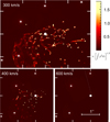 |
Fig. 4 Snapshots of the hydrodynamic simulations of the Wolf-Rayet stars (white asterisks) feeding Sgr A* (white disk) in the central parsec. The maps show density squared integrated along the line of sight in square-root scale, that is, [∫ρ2dz]1/2, i.e., the expected Brackett-γ flux. Each panel represents a simulation run with different wind speeds from IRS 16SW: 300 km s−1 (top), 400 km s−1 (bottom left), and 600 km s−1 (bottom right). The production of clumps on the scale shown here is dominated by IRS16 SW. The snapshots were created with Splash (Price 2007). |
5 Conclusions
New near-infrared IFU data from the Galactic center reveal a third object resembling G1 and G2, moving along (roughly) the same orbit but 18 years later. Given that probabilistic arguments de facto exclude finding three stellar sources in such a configuration, the new data render a stellar model – at least for these three sources – very unlikely. A much better picture is that of a G1–2–3 gas streamer apparently originating from the young, massive binary star IRS 16SW in the CW disk. The dominant differences between the orbits of the three gas clouds are the pericenter times and orientations of the (initial) orbital ellipses in their planes. These change systematically and synchronously with the motion of IRS 16SW. We conclude that G1–2–3 most likely originates from the winds of that star. Updated hydrodynamic simulations, accounting for lower wind velocities as they occur around binaries, show that IRS 16SW may well be able to produce clumps and filaments of gas that can reach Sgr A*.
Acknowledgements
We are very grateful to our funding agency MPG, to ESO and the Paranal staff, and to the many scientific and technical staff members in our institutions, who helped to design, build, test, commission and operate ERIS. Based on observations collected at the European Southern Observatory under the ESO programs listed in Appendix A. The research of D.C. has been funded by the Alexander von Humboldt Foundation. JC acknowledges financial support from ANID – FONDECYT Regular 1211429 and 1251444, and Millennium Science Initiative Program NCN2023_002. The research of TP was supported by an advanced ERC grant ‘multijets’.
References
- Agol, E. 2000, ApJ, 538, L121 [Google Scholar]
- Baganoff, F. K., Maeda, Y., Morris, M., et al. 2003, ApJ, 591, 891 [Google Scholar]
- Bartko, H., Martins, F., Fritz, T. K., et al. 2009, ApJ, 697, 1741 [Google Scholar]
- Bartos, I., Haiman, Z., Kocsis, B., & Márka, S. 2013, Phys. Rev. Lett., 110, 221102 [Google Scholar]
- Bonnet, H., Ströbele, S., Biancat-Marchet, F., et al. 2003, Proc. SPIE 4839, 329 [Google Scholar]
- Bower, G. C., Wright, M. C. H., Falcke, H., & Backer, D. C. 2003, ApJ, 588, 331 [Google Scholar]
- Bower, G. C., Markoff, S., Dexter, J., et al. 2015, ApJ, 802, 69 [Google Scholar]
- Calderón, D., Ballone, A., Cuadra, J., et al. 2016, MNRAS, 455, 4388 [Google Scholar]
- Calderón, D., Cuadra, J., Schartmann, M., et al. 2018, MNRAS, 478, 3494 [CrossRef] [Google Scholar]
- Calderón, D., Cuadra, J., Schartmann, M., et al. 2020a, MNRAS, 493, 447 [Google Scholar]
- Calderón, D., Cuadra, J., Schartmann, M., Burkert, A., & Russell, C. M. P. 2020b, ApJ, 888, L2 [Google Scholar]
- Calderón, D., Cuadra, J., Russell, C. M. P., et al. 2025, A&A, 693, A180 [NASA ADS] [CrossRef] [EDP Sciences] [Google Scholar]
- Chuard, D., Terrier, R., Goldwurm, A., et al. 2018, A&A, 610, A34 [NASA ADS] [CrossRef] [EDP Sciences] [Google Scholar]
- Ciurlo, A., Campbell, R. D., Morris, M. R., et al. 2020, Nature, 577, 337 [Google Scholar]
- Clavel, M., Terrier, R., Goldwurm, A., et al. 2013, A&A, 558, A32 [NASA ADS] [CrossRef] [EDP Sciences] [Google Scholar]
- Clénet, Y., Rouan, D., Gratadour, D., et al. 2005, A&A, 439, L9 [NASA ADS] [CrossRef] [EDP Sciences] [Google Scholar]
- Crumley, P., & Kumar, P. 2013, MNRAS, 436, 1955 [Google Scholar]
- Cuadra, J., Nayakshin, S., Springel, V., & Di Matteo, T. 2006, MNRAS, 366, 358 [NASA ADS] [CrossRef] [Google Scholar]
- Cuadra, J., Nayakshin, S., & Martins, F. 2008, MNRAS, 383, 458 [NASA ADS] [Google Scholar]
- Cuadra, J., Nayakshin, S., & Wang, Q. D. 2015, MNRAS, 450, 277 [CrossRef] [Google Scholar]
- Davies, R., Absil, O., Agapito, G., et al. 2023, A&A, 674, A207 [NASA ADS] [CrossRef] [EDP Sciences] [Google Scholar]
- DePoy, D. L., Pepper, J., Pogge, R. W., et al. 2004, ApJ, 617, 1127 [Google Scholar]
- Eckart, A., & Genzel, R. 1996, Nature, 383, 415 [NASA ADS] [CrossRef] [Google Scholar]
- Eckart, A., Mužić, K., Yazici, S., et al. 2013, A&A, 551, A18 [NASA ADS] [CrossRef] [EDP Sciences] [Google Scholar]
- Eisenhauer, F., Abuter, R., Bickert, K., et al. 2003, in Proc. SPIE, 4841, Instrument Design and Performance for Optical/Infrared Ground-based Telescopes, eds. M. Iye, & A. F. M. Moorwood, 1548 [Google Scholar]
- Eisenhauer, F., Genzel, R., Alexander, T., et al. 2005, ApJ, 628, 246 [Google Scholar]
- Ghez, A. M., Klein, B. L., Morris, M., & Becklin, E. E. 1998, ApJ, 509, 678 [NASA ADS] [CrossRef] [Google Scholar]
- Ghez, A., Duchêne, G., Matthews, K., et al. 2003, ApJ, 586, L127 [NASA ADS] [CrossRef] [Google Scholar]
- Ghez, A. M., Hornstein, S. D., Lu, J. R., et al. 2005, ApJ, 635, 1087 [NASA ADS] [Google Scholar]
- Ghez, A., Salim, S., Weinberg, N. N., et al. 2008, ApJ, 689, 1044 [Google Scholar]
- Gillessen, S., Eisenhauer, F., Trippe, S., et al. 2009, ApJ, 692, 1075 [NASA ADS] [CrossRef] [Google Scholar]
- Gillessen, S., Genzel, R., Fritz, T. K., et al. 2012, Nature, 481, 51 [Google Scholar]
- Gillessen, S., Genzel, R., Fritz, T. K., et al. 2013, ApJ, 774, 44 [NASA ADS] [CrossRef] [Google Scholar]
- Gillessen, S., Plewa, P. M., Eisenhauer, F., et al. 2017, ApJ, 837, 30 [Google Scholar]
- Gillessen, S., Plewa, P. M., Widmann, F., et al. 2019, ApJ, 871, 126 [NASA ADS] [CrossRef] [Google Scholar]
- GRAVITY Collaboration (Abuter, R., et al.) 2022, A&A, 657, L12 [NASA ADS] [CrossRef] [Google Scholar]
- Gravity Collaboration (Straub, O., et al.) 2023, A&A, 672, A63 [NASA ADS] [CrossRef] [EDP Sciences] [Google Scholar]
- Gravity Collaboration (Abd El Dayem, K., et al.) 2024, A&A, 692, A242 [NASA ADS] [CrossRef] [EDP Sciences] [Google Scholar]
- Guillochon, J., Loeb, A., MacLeod, M., & Ramirez-Ruiz, E. 2014, ApJ, 786, L12 [Google Scholar]
- Hobbs, A., Read, J., Power, C., & Cole, D. 2013, MNRAS, 434, 1849 [Google Scholar]
- Jia, S., Xu, N., Lu, J. R., et al. 2023, ApJ, 949, 18 [NASA ADS] [CrossRef] [Google Scholar]
- Lenzen, R., Hofmann, R., Bizenberger, P., & Tusche, A. 1998, Proc. SPIE, 3354, 606 [Google Scholar]
- Levin, Y., & Beloborodov, A. M. 2003, ApJ, 590, L33 [NASA ADS] [CrossRef] [Google Scholar]
- Lu, J. R., Ghez, A. M., Hornstein, S. D., et al. 2009, ApJ, 690, 1463 [NASA ADS] [CrossRef] [Google Scholar]
- Madigan, A.-M., McCourt, M., & O’Leary, R. M. 2017, MNRAS, 465, 2310 [Google Scholar]
- Marrone, D. P., Moran, J. M., Zhao, J.-H., & Rao, R. 2006, ApJ, 640, 308 [NASA ADS] [CrossRef] [Google Scholar]
- Marrone, D. P., Moran, J. M., Zhao, J.-H., & Rao, R. 2007, ApJ, 654, L57 [NASA ADS] [CrossRef] [Google Scholar]
- Martins, F., Trippe, S., Paumard, T., et al. 2006, ApJ, 649, L103 [NASA ADS] [CrossRef] [Google Scholar]
- Martins, F., Genzel, R., Hillier, D. J., et al. 2007, A&A, 468, 233 [NASA ADS] [CrossRef] [EDP Sciences] [Google Scholar]
- McCourt, M., & Madigan, A.-M. 2016, MNRAS, 455, 2187 [Google Scholar]
- Meyer, F., & Meyer-Hofmeister, E. 2012, A&A, 546, L2 [NASA ADS] [CrossRef] [EDP Sciences] [Google Scholar]
- Miralda-Escudé, J. 2012, ApJ, 756, 86 [CrossRef] [Google Scholar]
- Murray-Clay, R. A., & Loeb, A. 2012, Nat. Commun., 3, 1049 [NASA ADS] [CrossRef] [Google Scholar]
- Naoz, S., Will, C. M., Ramirez-Ruiz, E., et al. 2020, ApJ, 888, L8 [Google Scholar]
- Narayan, R., Özel, F., & Sironi, L. 2012, ApJ, 757, L20 [Google Scholar]
- Ott, T. 2025, QfitsView, https://www.mpe.mpg.de/~ott/QFitsView/ [Google Scholar]
- Ott, T., Eckart, A., & Genzel, R. 1999, ApJ, 523, 248 [NASA ADS] [CrossRef] [Google Scholar]
- Paumard, T., Genzel, R., Martins, F., et al. 2006, ApJ, 643, 1011 [NASA ADS] [CrossRef] [Google Scholar]
- Pfuhl, O., Gillessen, S., Eisenhauer, F., et al. 2015, ApJ, 798, 111 [NASA ADS] [CrossRef] [Google Scholar]
- Phifer, K., Do, T., Meyer, L., et al. 2013, ApJ, 773, L13 [NASA ADS] [CrossRef] [Google Scholar]
- Plewa, P. M., Gillessen, S., Pfuhl, O., et al. 2017, ApJ, 840, 50 [NASA ADS] [CrossRef] [Google Scholar]
- Ponti, G., De Marco, B., Morris, M. R., et al. 2015, MNRAS, 454, 1525 [NASA ADS] [CrossRef] [Google Scholar]
- Price, D. J. 2007, PASA, 24, 159 [Google Scholar]
- Price, D. J., Wurster, J., Tricco, T. S., et al. 2018, PASA, 35, e031 [Google Scholar]
- Prodan, S., Antonini, F., & Perets, H. B. 2015, ApJ, 799, 118 [Google Scholar]
- Quataert, E., & Gruzinov, A. 2000, ApJ, 539, 809 [NASA ADS] [CrossRef] [Google Scholar]
- Quataert, E., Narayan, R., & Reid, M. J. 1999, ApJ, 517, L101 [NASA ADS] [CrossRef] [Google Scholar]
- Reid, M. J., & Brunthaler, A. 2020, ApJ, 892, 39 [Google Scholar]
- Ressler, S. M., Quataert, E., & Stone, J. M. 2018, MNRAS, 478, 3544 [NASA ADS] [CrossRef] [Google Scholar]
- Rousset, G., Lacombe, F., Puget, P., et al. 1998, Proc. SPIE, 3353, 508 [Google Scholar]
- Schartmann, M., Ballone, A., Burkert, A., et al. 2015, ApJ, 811, 155 [Google Scholar]
- Schödel, R., Ott, T., Genzel, R., et al. 2002, Nature, 419, 694 [Google Scholar]
- Scoville, N., & Burkert, A. 2013, ApJ, 768, 108 [NASA ADS] [CrossRef] [Google Scholar]
- Stephan, A. P., Naoz, S., Ghez, A. M., et al. 2016, MNRAS, 460, 3494 [NASA ADS] [CrossRef] [Google Scholar]
- Vishniac, E. T. 1994, ApJ, 428, 186 [Google Scholar]
- von Fellenberg, S. D., Gillessen, S., Stadler, J., et al. 2022, ApJ, 932, L6 [NASA ADS] [CrossRef] [Google Scholar]
- Wang, Q. D., Nowak, M. A., Markoff, S. B., et al. 2013, Science, 341, 981 [NASA ADS] [CrossRef] [Google Scholar]
- Witzel, G., Ghez, A. M., Morris, M. R., et al. 2014, ApJ, 796, L8 [NASA ADS] [CrossRef] [Google Scholar]
- Witzel, G., Sitarski, B. N., Ghez, A. M., et al. 2017, ApJ, 847, 80 [NASA ADS] [CrossRef] [Google Scholar]
- Yelda, S., Ghez, A. M., Lu, J. R., et al. 2014, ApJ, 783, 131 [Google Scholar]
- Yuan, F., & Narayan, R. 2014, ARA&A, 52, 529 [Google Scholar]
- Yuan, F., Quataert, E., & Narayan, R. 2003, ApJ, 598, 301 [Google Scholar]
The name G3 has already been used by Ciurlo et al. (2020) for another, unrelated gaseous object.
Appendix A Data
Integral-field spectroscopy observations used for G2t.
Appendix B Orbital elements
We use the classical orbital elements for the non-Keplerian orbits in the sense of osculating elements. They are semimajor axis a, eccentricity e, inclination i, position angle ascending of the ascending node Ω, longitude of the pericenter ω and epoch of pericenter passage tP. The mass M of Sgr A* and its distance R0 are kept fixed. For the individual fits, we include the drag force parameter (Gillessen et al. 2019) as a free parameter for G2, and use the resulting best-fit value as fixed quantity for the much less constrained G1 and G2t fits. The uncertainties are the formal fit uncertainties, rescaled such the reduced χ2 of each fit is 1. The orbit of G1 with our data is only poorly constrained, especially in a and e, where the formal uncertainties don’t properly represent the posterior space. Comparing with Witzel et al. (2017) and/or including their data for increased phase coverage in our fits, leads to a semimajor axis value comparable with that of G2, and an eccentricity of around e = 0.98.
Orbit parameters for the individual orbit fits.
Orbit parameters for the common orbit fit.
Appendix C Additional illustration
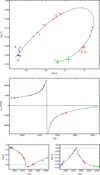 |
Fig. C.1 Alternative representation of the combined orbit fit for G1, G2, and G2t. The data from G1 (green) and G2t (blue) have been corrected for the differences in the respective orbits to the G2 orbit and plotted on top of the G2 orbit and data (red). |
Appendix D Clump mass function from the test simulations
Here we present the clump mass functions from our test simulations, at the present time and considering a central sphere of radius one arcsecond only. We first use splash to limit the computational domain to the inner arcsecond and output a uniformly sampled cubic grid of 1283 cells. On that grid we search for structures using the astrodendro package2. There are two parameters that control how a clump is defined, namely the number of sigmas above mean density for determining the density threshold, and the minimum number of cells that can constitute a clump. By visual inspection we found that making both parameters equal to 10 gave the best results.
Figure D.1 shows the mass function for the simulations with wind velocity 300 and 400 km s−1, while for the model with 600 km s−1 no clumps were formed. In the two models with the slowest wind there are 21 and four clumps above 3M⊕. While the clump numbers change for different parameters of the dendrogram algorithm, in particular at the low-mass end, the qualitative result is robust.
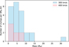 |
Fig. D.1 Clump mass functions from our test simulations. These consider the inner arc second only and are taken from the snapshots corresponding to the present time. Results are shown for the runs with wind velocities for IRS 16SW of 300 and 400 km s−1. The control run with 600 km s−1 did not yield a single clump. |
All Tables
All Figures
|
Fig. 1 G2t in the ERIS integral-field data from June/July 2024. Top left: continuum image showing the S-stars. Top right: Background-subtracted line map centered at 2.173 µm, corresponding to Brackett-γ + 1000 km/s. G2t stands out. Bottom left: example of a pixel selection (on – green, off – red) for extracting the G2t spectrum overlaid on the continuum map. Bottom right: Resulting spectrum showing a strong emission line at 2.173 µm. |
| In the text | |
|
Fig. 2 Orbits and data of G1, G2, and G2t, fit under the constraint that they share the same orbital plane, semimajor axis, and eccentricity. Top: on-sky appearance of the two orbits. Middle: radial velocities. Bottom: spatial coordinates as a function of time. The non-Keplerian shapes result from the drag force acting on G2 and G2t when they are close to Sgr A*. |
| In the text | |
|
Fig. 3 Left: position–velocity diagram extracted from the June/July-2024 data cube, using a curved slit along the orbital trace of G2t. The emission of G2t is concentrated around (−300 mas, +1000km/s). Similar to G2, G2t seems to be followed by a tail, indicative of even more material flowing along the G1–2–3 path. Right: same diagram for G2 extracted from the 2008 data cube (from Gillessen et al. 2019) for comparison. |
| In the text | |
|
Fig. 4 Snapshots of the hydrodynamic simulations of the Wolf-Rayet stars (white asterisks) feeding Sgr A* (white disk) in the central parsec. The maps show density squared integrated along the line of sight in square-root scale, that is, [∫ρ2dz]1/2, i.e., the expected Brackett-γ flux. Each panel represents a simulation run with different wind speeds from IRS 16SW: 300 km s−1 (top), 400 km s−1 (bottom left), and 600 km s−1 (bottom right). The production of clumps on the scale shown here is dominated by IRS16 SW. The snapshots were created with Splash (Price 2007). |
| In the text | |
|
Fig. C.1 Alternative representation of the combined orbit fit for G1, G2, and G2t. The data from G1 (green) and G2t (blue) have been corrected for the differences in the respective orbits to the G2 orbit and plotted on top of the G2 orbit and data (red). |
| In the text | |
|
Fig. D.1 Clump mass functions from our test simulations. These consider the inner arc second only and are taken from the snapshots corresponding to the present time. Results are shown for the runs with wind velocities for IRS 16SW of 300 and 400 km s−1. The control run with 600 km s−1 did not yield a single clump. |
| In the text | |
Current usage metrics show cumulative count of Article Views (full-text article views including HTML views, PDF and ePub downloads, according to the available data) and Abstracts Views on Vision4Press platform.
Data correspond to usage on the plateform after 2015. The current usage metrics is available 48-96 hours after online publication and is updated daily on week days.
Initial download of the metrics may take a while.