| Issue |
A&A
Volume 707, March 2026
|
|
|---|---|---|
| Article Number | A287 | |
| Number of page(s) | 11 | |
| Section | Extragalactic astronomy | |
| DOI | https://doi.org/10.1051/0004-6361/202556028 | |
| Published online | 16 March 2026 | |
Effect of the large-scale cosmic web environment on the X-ray-emitting circumgalactic medium
1
Max Planck Institute for Extraterrestrial Physics (MPE), Gießenbachstraße 1, 85748 Garching, Munich, Germany
2
Kavli IPMU (WPI), UTIAS, The University of Tokyo, Kashiwa, Chiba 277-8583, Japan
3
Department of Physics, Yale University, New Haven, CT 06520, USA
4
Department of Astronomy, Yale University, New Haven, CT 06520, USA
5
European Southern Observatory, Karl-Schwarzschild-Straße 2, 85748 Garching, Munich, Germany
6
Institut d’Astrophysique de Paris, 98bis Bd Arago, 75014 Paris, France
7
INAF-Osservatorio Astronomico di Brera, Via E. Bianchi 46, I-23807 Merate (LC), Italy
★ Corresponding author: This email address is being protected from spambots. You need JavaScript enabled to view it.
Received:
19
June
2025
Accepted:
1
February
2026
Abstract
Aims. The hot circumgalactic medium (CGM), probed by X-ray observations, plays a central role in understanding gas flows that drive a galaxy’s evolution. While CGM properties have been widely studied, the influence of a galaxy’s large-scale cosmic environment on the hot gas content remains less explored. We investigate how the large-scale cosmic web affects the X-ray surface brightness (XSB) profiles of galaxies in the context of cosmological simulations.
Methods. We used our novel IllustrisTNG-based lightcone, first developed in our previous work and spanning 0.03 ≤ z ≤ 0.3, to generate self-consistent mock X-ray observations, using intrinsic gas cell information. We applied the filament-finder DisPerSE on the galaxy distributions to identify cosmic filaments within the lightcone. We classified central galaxies into five distinct large-scale environment (LSE) categories: clusters and massive groups, cluster outskirts, filaments, filament-void transition regions, and voids and walls.
Results. We find that the X-ray surface brightness profiles (XSB) of central galaxies of dark matter halos in filaments with M200 m > 1012 M⊙ are X-ray brighter than those in voids and walls, with 20 − 45% deviations in the radial range of (0.3 − 0.5)×R200 m. We investigated the source of this enhancement and found that filament galaxies have higher average gas densities, temperatures, and metallicities than void and wall galaxies.
Conclusions. Our results demonstrate that the impact of the large-scale cosmic environment is imprinted on the hot CGM’s X-ray emission. Future theoretical works studying the effects of assembly history, connectivity, and gas accretion on galaxies in filaments and voids would help further our understanding of the impact of the environment on X-ray observations.
Key words: galaxies: evolution / galaxies: halos / large-scale structure of Universe / X-rays: galaxies
© The Authors 2026
 Open Access article, published by EDP Sciences, under the terms of the Creative Commons Attribution License (https://creativecommons.org/licenses/by/4.0), which permits unrestricted use, distribution, and reproduction in any medium, provided the original work is properly cited.
This article is published in open access under the Subscribe to Open model.
Open access funding provided by Max Planck Society.
1. Introduction
Observational and theoretical studies show that galaxy properties, such as stellar mass, star formation rate, and gas content, vary across different large-scale environments (LSEs). The galaxies close to groups and clusters, which form the nodes of the cosmic web, are more likely to be elliptical, red, and have suppressed star formation, compared to their less crowded “field” counterparts that tend to be spiral, blue, and actively forming stars (Dressler 1980; Butcher & Oemler 1984; Dressler et al. 1997; Lewis et al. 2002; Blanton et al. 2005; Alpaslan et al. 2015; Pasquali & Nachname 2015; Shimakawa et al. 2021). Additionally, galaxies infalling into clusters via cosmic filaments are systematically more quenched than their counterparts from other isotropic directions (see, e.g., Martínez et al. 2016; Einasto et al. 2018; Salerno et al. 2019; Gouin et al. 2020). Simulations show that the gas content of galaxies located as far as out to three times the virial radius (Cen et al. 2014; Arthur et al. 2019; Mostoghiu et al. 2021) to five times the virial radius (Bahé et al. 2013) of the group and cluster centres is gas-depleted compared to their counterparts in the field, as also reaffirmed by observations (e.g., Tanaka et al. 2004; Catinella et al. 2013; Cortese et al. 2011). Similar trends of higher gas depletion, higher quiescent fraction, and stellar mass also hold for galaxies closer to the cosmic filament spines (Malavasi et al. 2017; Laigle et al. 2018; Sarron et al. 2019; Bonjean et al. 2020; Winkel et al. 2021; Hoosain et al. 2024).
The hot CGM is the diffuse gas that surrounds galaxies, playing a crucial role in regulating the growth and evolution of the galaxy (see Tumlinson et al. 2017 and Faucher-Giguère & Oh 2023 for a review). The hot gas (T ≳ 106 K) reservoir hosted by the CGM is crucial for replenishing the cold gas consumed for star formation (Fox & Davé 2017; Wang et al. 2022). The ability of halos to retain or deplete their cold gas in an intrafilamentary environment has been shown to correlate with stellar mass in HI studies (see, e.g., Kleiner et al. 2017; Odekon et al. 2018; Hoosain et al. 2024). From these HI studies, the emerging picture is that mass plays a crucial role in determining whether a galaxy can retain or further accrete gas from the cosmic web, or whether it is more vulnerable to stripping and supply truncation. More massive galaxies (M★ > 1011 M⊙) retain and accrete gas from the surrounding filament due to their deeper gravitational potentials; however, lower mass galaxies (M★ < 1010.5 M⊙) are more susceptible to gas-depleting processes, such as stripping and detachment. However, there is an overall lack of understanding related to how the hot gas content around galaxies, as probed by the CGM, is impacted by filaments, voids, and nodes. This motivates the need to explore whether the hot CGM, traced through X-ray emission, encodes information about a galaxy’s cosmic web environment.
In the lambda cold dark matter (ΛCDM) Universe, the existence of the cosmic web follows from the initial fluctuations in the primordial density field, whose evolution is dictated by gravity in an expanding Universe. The anisotropic nature of gravitational collapse leads to the formation of high-density peaks that are the nodes that host today’s galaxy clusters, while the expansive network of bridges between these nodes forms a large-scale web dominated by filaments, which demarcate the underdense voids (Peebles 2020). The theoretical formulation of the existence and evolution of the cosmic web (Bond et al. 1996) has been confirmed by all large N-body simulations of structure formation in a ΛCDM Universe (e.g., Klypin & Shandarin 1983; Springel et al. 2006; Popping et al. 2009; Angulo et al. 2012; Habib et al. 2012; Poole et al. 2015). The existence of filaments, clusters, and voids is also reaffirmed with advances in spectroscopic surveys, with increasing resolution and depth, which have allowed us to observationally map the cosmic web. A unified approach to jointly study the cosmic web, as traced by galaxies, is possible with exquisite detail up to redshift z ≈ 0.9 with surveys such as the CfA Redshift Survey (de Lapparent et al. 1986), SDSS (York et al. 2000), 2dFGRS (Colless et al. 2001), 6dFGS (Jones et al. 2009), GAMA Driver et al. (2011), Vipers (Guzzo et al. 2014), 2MASS (Huchra et al. 2012), and COSMOS (Scoville et al. 2007). This is being further explored at higher redshifts of z ≈ 2, close to the peak epoch of star formation, with ongoing and upcoming Stage-4 surveys such as Euclid (Laureijs et al. 2011), PFS (Takada et al. 2014), and 4MOST (De Jong et al. 2012).
Studies using simulations find that cosmic filaments dominate the mass budget, occupying 50% of the total mass of the cosmic web, with mean overdensities δ ∼ 10 (Cautun et al. 2014), while the underdense voids, δ ∼ −0.8, are the most voluminous component of the cosmic web (Sheth & Van De Weygaert 2004). Cui et al. (2018) show that the gas component is the dominant baryonic tracer of cosmic filaments, hosting the warm-hot intergalactic medium (WHIM) gas phase (Galárraga-Espinosa et al. 2021). The WHIM gas can be accreted onto the halos resulting in the denser circumgalactic medium (CGM) gas phase (nH ≳ 10−4 cm−3; see the categorization in Martizzi et al. 2019). Inversely, CGM gas around halos might be ejected due to feedback effects or undergo stripping due to ram-pressure inside filaments (Benítez-Llambay et al. 2013; Winkel et al. 2021). Liao & Gao (2019) show that up to 30% of the gas accreting onto galaxies residing in filaments is pre-processed and they also have higher baryon fractions compared to the field galaxies (e.g., see also Singh et al. 2020). Thus, the CGM, as probed by X-rays, is an interesting avenue for testing these environment-driven gas processes.
In this work, we use an IllustrisTNG-based lightcone from Shreeram et al. (2025b, a), called LC-TNGX, to study the impact of the LSE on the hot gas properties of galaxies. Isolating the impact of the large-scale environment (LSE) is complicated by the fact that various mechanisms, both gravitational and hydrodynamic, act on galaxies simultaneously. In particular, local overdensity and galaxy hierarchy (central vs. satellite) also impact galaxy properties (Pasquali & Nachname 2015; O’Kane et al. 2024; Rodríguez-Medrano et al. 2024). The latter effect can be accounted for by separately studying the trends of central and satellite galaxy properties (Yu et al. 2025). The former effect of local overdensity (or crowdedness of the environment) is related to the degeneracies between different cosmic web environments’ local and global overdensities (Hahn et al. 2007; Cautun et al. 2014; O’Kane et al. 2024). As the local overdensity correlates with the halo mass function, where massive halos reside in high-density regions (Tinker et al. 2011; Wang et al. 2018; Wechsler & Tinker 2018), this work accounts for local density effects by studying the impact of the LSE in halo-mass bins. In this way, we can additionally distinguish the effect of the stellar-to-halo-mass relation (SHMR) from that of the LSE (e.g., see Wechsler & Tinker 2018).
The paper is organized as follows. We describe the LC-TNGX and the procedure we used to self-consistently generate mock X-ray observations within the LC-TNGX, using the gas cell information in Sect. 2.1. We detail our application of DisPerSe to the galaxy distribution, aiming to identify the cosmic filaments within LC-TNGX, in Sect. 2.2. We classify the central galaxies in different LSE: clusters and groups, galaxies in clusters and group outskirts, galaxies in filaments, galaxies in the filament-void transition region, and galaxies in voids and walls in Sect. 2.3. Section 3 presents the main results of this work on how the XSB profiles are affected by the galaxies in different LSE. We interpret our findings in Sect. 4 and report our conclusions in Sect. 5.
2. Methods
This section outlines the data products used to study the impact of the LSE on the hot CGM. More precisely, Sect. 2.1 describes the TNG300 X-ray lightcone (LC-TNGX), Sect. 2.2 describes the filament catalogue obtained within the LC-TNGX using DisPerSE, and lastly, Sect. 2.3 describes the classifications of the LC-TNGX halos into their LSE categories.
2.1. The TNG300 X-ray lightcone: LC-TNGX
In this work, we model the hot gas emission using the TNG300 hydrodynamical simulations (Pillepich et al. 2018; Marinacci et al. 2018; Naiman et al. 2018; Nelson et al. 2015; Springel et al. 2018). We used TNG3001 to construct a lightcone, using the LightGen code2 and generated mock X-ray observations (LC-TNGX), which is presented in Shreeram et al. (2025b) and applied to eROSITA data in Shreeram et al. (2025a). Here, we summarize the most important features. Using the IllustrisTNG cosmological hydrodynamical simulation, with the box of side length 302.6 Mpc (Nelson et al. 2019, TNG300), we mapped the hot CGM around a wide range of halo masses embedded in the LSS. TNG300 contains 25003 dark matter particles, with a baryonic mass resolution of 1.1 × 10⁷ M⊙, a comoving value of the adaptive gas gravitational softening length for gas cells of 370 comoving parsec, gravitational softening of the collisionless component of 1.48 kpc, and dark matter mass resolution of 5.9 × 10⁷ M⊙. The TNG simulations adopt the cosmological parameters from Planck Collaboration XIII 2016. LC-TNGX is constructed with the box remap technique (Carlson & White 2010) and spans across redshifts of 0.03 ≲ z ≲ 0.3; this range was motivated by the initial MW-mass scale of the hot CGM observations (e.g., Comparat et al. 2022; Chadayammuri et al. 2022; Zhang et al. 2024). It goes out to 1231 comoving Mpc (cMpc) along the x-axis, subtending an area of 47.28 deg2 on the sky in the y-z plane. There are 22 snapshots within the observationally motivated redshift range of 0.03 ≤ z ≤ 0.3.
The physical properties of the distinct halos and subhalos within the TNG300 lightcone were obtained by the friends-of-friends (FoF) and SUBFIND algorithms (Springel et al. 2001; Dolag et al. 2009). SUBFIND detects gravitationally bound substructures, equivalent to galaxies in observations, and also provides us with a classification of subhalos into centrals and satellites, where centrals are the most massive substructure within a distinct FoF halo.
This paper focuses its analysis on studying the average XSB profiles from central galaxies in halo-mass bins. Therefore, we used the FoF groups, whose centres are defined as the most bound particle within the central subhalo as found by the SUBFIND algorithm. We did not include satellites, since their stacked XSB profiles are dominated by the hot gas emission of their more massive host halos, rather than the intrinsic CGM of the satellites themselves. Segregating satellites by environment would therefore not directly probe their own hot gas content, but instead the emission of their nearby massive companions. This effect has been quantified in detail in Shreeram et al. (2025b), where we show that including satellites primarily adds a flat background component to the stacked profiles at large radii, driven by group- and cluster-mass host halos. Since the aim of this work is to study the XSB of galaxies as a function of environment, we focussed exclusively on centrals, for which the measured signal can be directly interpreted in terms of their own halo gas content.
The X-ray photons are simulated within the LC-TNGX in the 0.5 − 2.0 keV intrinsic band with pyXsim (ZuHone & Hallman 2016), which is based on PHOX (Biffi et al. 2013), by assuming an input emission model where the hot X-ray emitting gas is in collisional ionization equilibrium. The X-ray emissivity, ϵ, in turn depends on the gas mass density, ρ, temperature, T, and the metallicity of the gas, Zmet (Lovisari et al. 2021), as follows
 (1)
(1)
where ne and np are the number densities of the electron and protons, which are related to the gas mass density ρ = μmp(ne + np). Here, μ and mp are the mean molecular weight and the proton mass, respectively. Λ(T, Zmet) is the cooling function of the hot gas, which depends on the emission mechanism in the considered energy window3. The spectral model computations of hot plasma use the Astrophysical Plasma Emission Code, APEC4 code (Smith et al. 2001), with atomic data from ATOMDB v3.0.9 (Foster et al. 2012) and solar abundance values from Asplund et al. (2009). This model uses the plasma temperature of the gas cells (in keV), the redshift, z, and metallicity. We have improved the mock X-ray generation from Shreeram et al. (2025b), where we assumed a constant metallicity of 0.3 Z⊙, to include the intrinsic TNG gas cell metallicity. Additionally, we also have updated the solar abundance values used from Anders & Grevesse (1989) to Asplund et al. (2009). We report no impact of these updates on the averaged XSB profiles. Nevertheless, these key improvements enable a more accurate and self-consistent estimate of the X-ray emission at the gas cell level throughout the lightcone.
The events are generated by assuming a telescope with an energy-independent collecting area of 1000 cm2 and an exposure time of 1000 ks. The photon list is generated in the observed frame of the X-ray-emitting gas cells and is corrected to rest-frame energies. Finally, the photons generated by the gas cells are projected onto the sky. We used the projected central galaxy positions and obtain the XSB profiles in the 0.5 − 2.0 keV band. We selected the X-ray events within R200m5 of the parent halo for obtaining the XSB profiles and we define these profiles as the intrinsic hot gas emission profiles. In this work, we tested the impact of the CGM environment on the XSB profiles, showing the distribution of X-ray events in the bottom panel of Fig. 1. For this purpose, we classified the cosmic web in the LC-TNGX into different LSEs, as further described in the following sections. We note that the aim of this work is to provide predictions that are independent of instrument-specific systematics by isolating the underlying theoretical behaviour driven by the LSE within LC-TNGX. As shown in Shreeram et al. (2025a), a meaningful comparison with observations requires carefully modeling the stellar mass, redshift, and halo-mass distributions of the corresponding observational sample. Although no suitable datasets currently exist, this situation is expected to change with the forthcoming wide-area spectroscopic surveys, such as 4MOST.
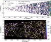 |
Fig. 1. TNG300 lightcone (LC-TNGX) built in Shreeram et al. (2025b) overplotted with the filaments, which are identified using the DisPerSe algorithm (Sect. ). The top panel shows the central galaxies in LC-TNGX that are classified into five distinct large-scale environments categories: (1) clusters in blue, (2) cluster outskirts in orange, (3) filaments in green, (4) filament-void transition region in red, and (5) voids and walls in purple, as defined in Sect. 2.3. The bottom panel zooms in on the lightcone, showing the X-ray events generated with pyXsim in the 0.5 − 2.0 keV energy band with the filaments depicted by the yellow-dashed lines. While the filaments are identified using the galaxy distribution, we show that the hot gas emitting X-ray events trace the cosmic web. This alignment validates the full pipeline used in this work, from the lightcone construction and X-ray map generation to filament identification. |
2.2. Extracting cosmic filaments in LC-TNGX using DisPerSE
The theoretical background of DisPerSE is provided in Sousbie (2011), Sousbie et al. (2011)6. Here, we summarize the most important details. DisPerSE deals with discrete datasets and provides the user with a geometric three-dimensional ridge, allowing for the classification of the cosmic web based on its topology. It is built on Morse and persistence theories, and it functions by first estimating the underlying density field, given an input galaxy distribution, using the Delaunay Tessellation Field Estimator (DTFE; Schaap & van de Weygaert 2000; Cautun & van de Weygaert 2011). The Delaunay tessellation is a triangulated space that represents a geometric assembly of cells, faces, edges, and vertices, mapping the entire volume of the galaxy distribution. The gradients of the DTFE density field, ρDTFE, provide the critical points: maxima, minima, and saddles, which are connected by field lines tangent to the gradient of ρDTFE. The filaments comprise connecting segments between the maxima of the density field, also known as CPmax or peaks and the saddle points.
The significance of a filament (or the persistence threshold) is estimated by the density contrast of the critical pair chosen to pass a certain signal-to-noise threshold. For a filament, this critical pair is between a CPmax and the saddle point. The noise level is defined relative to the root mean square of the significance values obtained from random sets of points. This thresholding eliminates less significant filaments, simplifying the Morse complex and retaining its most topologically robust features. The skeletons generated in this work use the 3σ persistence thresholds, following the careful calibration method presented in Galárraga-Espinosa et al. (2024). The galaxies above M★ > 109 M⊙ (83 297 galaxies) were used to build the skeleton, as shown in Fig. 1. This mass choice is motivated by matching typical galaxy mass limits in current observational surveys, as well as the resolution of the simulation used to construct the lightcone. We highlight that while the filament skeleton is constructed from DisPerSE, using the galaxy distribution, as shown by the top panel of Fig. 1, we find that the hot gas, as probed by the X-rays, also traces the cosmic web as shown in the bottom panel of Fig. 1. This alignment provides a compelling validation of the full pipeline used in this work, from the construction of the lightcone and the generation of X-ray maps to the identification of the filamentary network.
Fraction of galaxies in each halo-mass bin for each large-scale environment classification.
2.3. Classification of halos in LC-TNGX into different cosmic web environments
Given the skeleton from DisPerSE, the central galaxies in the LC-TNGX are divided into five mutually exclusive categories in a similar fashion as in Galárraga-Espinosa et al. (2023), also depicted in Fig. 1. We summarize the fraction of galaxies in each of these distinct LSE categories in Table 1 and we also illustrate the LSE classification of galaxies in Fig. 2, which are defined as follows.
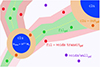 |
Fig. 2. Illustration of the classification of galaxies into different LSE categories within the LC-TNGX. The filament spines (yellow dashed lines) are extracted using the DisPerSe algorithm. The clusters, representing the nodes of the cosmic web, are defined as halos with masses of M200 m > 1013.5 M⊙. The dots represent central galaxies in different LSE, such as cluster outskirts (orange), filaments (green), filament-void transition region (red), and voids and walls (purple). |
-
Clusters and massive groups: The galaxy clusters and massive groups are defined as halos with M200 m > 1013.5 M⊙, with a radius R200 m, centred on the positions of the FoF halos.
-
Galaxies in cluster and group outskirts (clu-outgal): This category comprises of galaxies located (1 − 3)×R200 m from a cluster center. This radial range is motivated by Aung et al. (2023), who demonstrated that the gas accretion shock is located at approximately (1.5 − 3)×R200 m. This accretion shock leads to the onset of the galaxy quenched fraction, influenced by ram pressure and tidal stripping due to clusters, approaching the average value (e.g., Cen et al. 2014).
-
Galaxies in filaments (filgal): The cosmic filaments that are extracted by DisPerSe are defined as cylinders, with a radius of 1 cMpc (Wang et al. 2024), aligned along the spine of the filament skeleton identified by DisPerSe (Sect. 2.2). The central galaxies within the 1 cMpc cylinder of the filament spine are defined as galaxies in filaments.
-
Galaxies in the filament-voids+walls transition region (fil-voids transitgal): the central galaxies that are 1 − 3 cMpc away from the filament spine are categorized as galaxies in the passage between filaments and voids. This category is primarily designed to facilitate a smooth transition between galaxies located in the outskirts of filaments and those in voids and walls. For brevity, we also refer to this group of galaxies as the transition galaxies.
-
Galaxies in voids and walls (voids+wallgal): This category encompasses all the galaxies that do not fall in any of the above categories. These galaxies are also referred to as “field” galaxies. The galaxies in voids and walls have been combined due to a lack of information about the size of the void or wall, which is required to distinguish galaxies into these distinct categories.
We present the fraction of central galaxies in each of these distinct categories in Table 1; within LC-TNGX, of the 44 376 halos with M200 m ∈ 1011.5 − 13.5 M⊙, 8%, 11%, 22%, and 59% of the halos are located in cluster outskirts, filaments, filament-void transition region, and voids and walls, respectively.
We compare our findings on the fraction of filament galaxies with other literature works reporting the fraction of galaxies in filaments. Ganeshaiah Veena et al. (2019) find that 63% of the central galaxies are hosted by filaments; they use the EAGLE simulation and run the Bisous filament finder on the galaxy distribution. Using THETHREEHUNDRED project, Kuchner et al. (2022) found that 45% of the galaxies in filaments are feeding clusters (independent of the distance to the cluster). Navdha et al. (2025) used the Millennium simulation to show that 26% of the galaxies reside in the cosmic web at a halo mass of 1011 M⊙, going up to 50% at 1012.7 M⊙. However, these fractions encompass both central and satellite galaxies and they define the cosmic web in a different manner. We have taken extreme caution when directly comparing these values with the 11% of filament galaxies found in our work. As also highlighted by these works, the fraction of filament galaxies is affected by the following: (1) the box size and the volume of the simulation, which, in turn, affect the number of massive clusters in the LSS, which are different across the simulations discussed here; (2) different filament finding techniques (see, e.g., Cautun et al. 2013; Leclercq et al. 2016; Libeskind et al. 2018; Rost et al. 2020, for comparisons between different cosmic web identification methods); and (3) different cosmic web definitions, affecting in turn the resulting fraction of galaxies considered to be in filaments. Here, we perform, for the first time, this type of categorization for galaxies in a lightcone configuration (ranging across 0.03 ≤ z ≤ 0.3), which could display further deviations from galaxy categorizations in a cubic snapshot at a fixed redshift.
3. Effect of the environment on the X-ray surface brightness profiles of halos
The hot CGM emits in X-rays due to infalling gas within halos, which is shock-heated up to the virial temperatures of Tvir ≳ 5 × 10⁵ K (White & Rees 1978). We present the projected X-ray surface brightness profiles of halos for varying halo masses and cosmic web environments in Fig. 3. The increasing halo-mass bins (left to right) result in brighter XSB profiles, given that the gas is heated to higher virial temperatures (e.g., Comparat et al. 2022; Zhang et al. 2024).
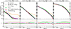 |
Fig. 3. X-ray surface brightness profiles (XSB) of halos located in different cosmic web environments in increasing halo-mass bins from left to right. The fraction of central galaxies in each mass bin (and each LSE category) is shown in Table 1. The bottom panel shows the significance (see Eq. 2) of the difference in the XSB in a given cosmic environment with respect to the others (see text for details). The shaded regions around each curve correspond to the uncertainty in the mean profile obtained by bootstrapping. |
We separated galaxies into the following different bins of halo mass: M200 m ∈ 1011.5 − 12 M⊙, M200 m ∈ 1012 − 12.5 M⊙, M200 m ∈ 1012.5 − 13 M⊙, and M200 m ∈ 1013 − 13.5 M⊙. These are hereafter referred to as the lowest, low, medium, and highest mass bins, respectively. For the lowest halo-mass bin (leftmost panel), the peak temperature of the gas within the halo is 0.03 − 0.09 keV (also shown later in Fig. 5), which is well below the 0.5 − 2 keV soft X-ray band considered here for measuring the XSB profiles. Therefore, the results of the XSB profiles corresponding to this lowest mass bin only probe the high-temperature end of the halos in the lowest halo-mass bin presented in the XSB profiles, which would explain their weak signal. Future studies that focus on a softer bandpass would allow for the full thermal emission of the lowest mass halos to be probed more effectively.
The different LSE considered are shown in Fig. 3: cluster outskirts (orange), filaments (green), filament-void transition region (red), and voids and walls (purple). The bottom panel of Fig. 3 shows the significance of the deviation of a given XSB profile, SX, i, in a defined LSE category with respect to all the other categories,  . Here, the subscript i signifies one among the five LSE categories defined in Sect. 2.3 (also shown by the colored lines in Fig. 3), while
  (with a tilde) is the XSB profile obtained by averaging over all the galaxies in the other LSE categories. The significance, σ, is defined as
 (2)
(2)
where δi and  are the uncertainties in the mean XSB profiles obtained from bootstrapping. A positive significance implies that a given SX, i is brighter at a given scale compared to its counterparts in other LSE, while the negative significance represents steeper or X-ray fainter profiles. Another useful metric we use to compare the observed differences in the XSB profiles in Fig. 4 is the percentage deviation, Δ, where
 (3)
(3)
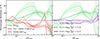 |
Fig. 4. Percentage deviations of the XSB profiles of halos located in filaments (green), compared to those in the filament-void transition region (left panel: red lines) and in voids and walls (right: purple lines). We also show the effect of varying the halo-mass bins, where the dotted lines represent the M200 m ∈ 1012 − 12.5 M⊙ halos, whereas the dashed and solid lines represent the M200 m ∈ 1012.5 − 13 M⊙ and M200 m ∈ 1013 − 13.5 M⊙ bins, respectively. We find that the XSB profiles of filgal are X-ray brighter in ∼(0.3 − 0.5)×R200 m by 20 − 45% with respect to the fil-voids transitgal and voids+wallgal populations. |
The following sections detail the trends observed in the XSB profiles in the different LSE categories. We present the effect of the LSE on the XSB profiles of halos in cluster outskirts in Sect. 3.1, with those of filaments, voids and walls given in Sect. 3.2.
3.1. Galaxies in cluster outskirts
The clu-outgal galaxy population probes the XSB profile of the halos located physically close to a cluster, shown by the orange lines in Fig. 3. Across all halo-mass bins (left to right), although notably more prominent at the lowest and low halo-mass bins, the XSB profiles from clu-outgal are significantly brighter than the mean XSB profile (without categorizing halos by their LSE). We attribute this striking feature of XSB profiles from clu-outgal to its close proximity to a cluster, where the emission from the intracluster medium (ICM) in the cluster outskirts begins to dominate the profile at these radii. We further quantified this effect in the significance plots in the bottom panel of Fig. 3. We show that the halos in the least massive bin are 2σ brighter at 0.2 R200 m. The significance is over 3σ at 0.7 R200 m for the low-halo-mass bin. For the medium and highest halo-mass bins considered here, the significance of the XSB profiles from clu-outgal being brighter than their counterparts in other LSE is < 3σ significant at all radii. We explain the lower significance of the highest halo-mass bins by the fact that more massive halos have comparable intrinsic X-ray brightness to their neighbouring cluster. Therefore, the cluster emission only dominates at large radii. Our results demonstrate that X-ray contamination from the cluster is a significant factor to consider when studying galaxies in the cluster outskirts using X-ray stacking experiments.
Cluster and group outskirts are special regions, where the gas in these halos is depleted due to gas stripping processes, as shown by simulations (e.g., Bahé et al. 2013; Cen et al. 2014) and observations (e.g., Tanaka et al. 2004; Catinella et al. 2013; Cortese et al. 2011). However, to measure the impact of such stripping processes on the average XSB profiles obtained in stacking experiments, it is necessary to accurately model out the contribution of the ICM emission from clusters. A key finding of our analysis here is to highlight that galaxies in cluster outskirts appear X-ray bright primarily because they reside within (and are illuminated by) the extended ICM, rather than due to their own gas properties. The elevated XSB signal in these environments reflects the surrounding cluster emission itself. As the local ICM contribution varies with both cluster mass and a galaxy’s distance from the cluster centre, assessing the observability of this effect in real data would require detailed, galaxy-by-galaxy modeling prior to stacking. We have left this type of modeling analysis to a future work, with the aim to recover the XSB of galaxies in cluster outskirts from the contamination of the nearby cluster emission. The following sections focus on the other LSE categories that are unaffected by cluster emission, as they are located far (> 3R200 m) from the cluster and group centres.
3.2. Galaxies in filaments and voids
We focus on the galaxies far away from clusters and massive groups, which are located in filaments, voids and walls, as well as the transition region in between them. The filgal, fil-voids transitgal, and voids+wallgal population are shown by the green, red, and purple lines in Fig. 3, respectively, with the bottom panel showing the significance of deviation compared to other LSE. We further examined these three categories in Fig. 4, which displays the absolute deviation in the XSB profiles for the low-, medium-, and high-halo-mass bins. We excluded the lowest halo-mass bin, M200 m ∈ 1011.5 − 12 M⊙, from this comparison, as there was no observable trend captured due to the high scatter in the measured XSB profiles. We quantified the deviation of the filament galaxies with respect to transition galaxies (left panel) and the void and wall galaxies (right panel).
We find that for all the halo-mass bins considered, the XSB profiles of filgal are X-ray brighter than the mean population between ∼(0.3 − 0.5)×R200 m by 20 − 45%. More precisely, Fig. 4 shows that the filament galaxies in the low-, medium-, and highest halo-mass bins are brighter than the mean XSB profile at different fractions of R200 m. For the low-halo-mass bin, the maximum mean deviation is 20% at ∼0.45 × R200 m, whereas for medium and highest halo-mass bins, the maximum mean deviation of 40% and 20% is at ∼0.3R200 m and ∼0.5R200 m, respectively.
Interestingly, we also find that the voids and walls, as well as the transition galaxies, are X-ray fainter than the mean XSB profiles. In the fil-voids transitgal case, for all halo-mass bins, the maximum mean deviation is between −(10 − 20)% at ∼(0.2 − 0.3)×R200 m. This trend becomes weaker for the voids+wallgal populations, where all the XSB profiles are fainter than the mean profiles by less than 10% across all halo-mass bins.
We delve deeper into understanding the non-negligible XSB excess in the filamentary galaxies with respect to those in voids and walls and the transition galaxies by exploring the primary quantities affecting the X-ray emission, which are the underlying thermodynamic quantities. This is further detailed in the following section.
4. Discussion on filament galaxies being X-ray brighter than the galaxies in voids and walls
We investigated the thermodynamic properties, such as density, ρ, temperature, T, and metallicity, Zmet, of the hot gas (T > 5 × 10⁵ K)7 around galaxies given the dependence of X-ray emission on the gas properties, as shown in Eq. (1). In Fig. 5, we present the radial profiles of ρ (top panel), T (middle panel), and Zmet (bottom panel) for galaxies in filaments, voids and walls, and the transitional region for increasing halo-mass bins (left to right columns). The thermodynamic profiles shown in Fig. 5 were computed using gas cell information combined in an emission and volume-weighted manner in 3D. The volume weighting accounts for the cell refinement criterion in the simulation. Indeed, the moving-mesh AREPO code is based on a fixed-mass threshold for the gas cells (Weinberger et al. 2020), leading to a broad distribution of cell volumes. Therefore, our volume-weighted results are independent of the irregular volumes of the Voronoi gas cells in the AREPO grid. Contrary to the more conventional mass-weighted average profiles, which are biased by the different gas cell volumes.
For the highest halo-mass bin in Fig. 5, we find that the mean T and Zmet radial profiles are approximately 10% higher in filament galaxies, compared to those in voids and walls and the transition population. The mean density profiles also show an enhancement at r > 0.2 R200 m. However, due to the significant scatter around the mean profiles across different environments (as also illustrated in Fig. 5 of Truong et al. 2023), these average trends alone are insufficient to robustly interpret the observed X-ray enhancement. To better explore the full variations across galaxy populations in different LSEs, we studied the probability distribution functions (PDFs) of the average thermodynamic properties of individual galaxies as a function of the halo mass.
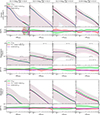 |
Fig. 5. Emission measure weighted gas mass density (top panel), temperature (middle panel), and metallicity (bottom panels) profiles together with their percentage deviations (corresponding bottom rows; see Eq. (3)) of halos located in different LSE in increasing halo-mass bins from left to right. The different cosmic environments considered here are filaments (green), filament-void transition region (red), and voids and walls (purple). The shaded regions show the 16th to 84th percentile distributions. |
Using the radial profiles presented in Fig. 5, we computed the emission-weighted average value of ρ, T, and Zmet for each galaxy within R200 m. In Fig. 6, we present the resulting normalized PDFs of these average thermodynamic quantities as a function of halo mass. The top, middle, and bottom panels correspond to the two-dimensional PDFs of ρ–M200 m, T–M200 m, and Zmet–M200 m, respectively. The first three columns present the normalized PDFs for galaxies residing in filaments (left), the filament-void transition region (middle), and voids and walls (right). The last two columns display the fractional difference in the PDFs relative to the filament population. Column four compares the transition population to filaments, and column five compares the voids and walls to filaments. The colour bars in the ratio panels indicate the relative suppression (blue) or enhancement (red) with respect to the filament galaxies. Across all three thermodynamic quantities, filament galaxies exhibit systematic enhancements compared to other large-scale environments. More specifically, galaxies in filaments are up to a factor of 6 − 9× more likely to have higher gas densities, 4 − 14× more likely to have higher temperatures, and 8 − 14× more likely to have higher metallicities than galaxies in transition regions and those in void and wall regions, respectively. These differences are especially pronounced in the medium-to-highest halo mass range (1012.5 M⊙ < M200 m < 1013.5 M⊙), where the contrast between environments is strongest. Within this mass bin, the PDF ratios between filament galaxies and those in voids and walls or transition regions are, on average, higher by factors of 40–70% across all thermodynamic quantities. This comparative study of the gas properties that directly affect X-ray emissivity is crucial for a better understanding of the results in Fig. 4.
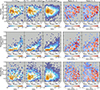 |
Fig. 6. Normalized probability distribution functions of gas mass density, ρ (top row), temperature, T (middle row), and metallicity, Zmet (bottom row), as a function of the halo mass. The population of galaxies in filaments (1825), filament-void transition region (3434), and voids and walls (10 183) is shown in the first three columns, respectively. The last two columns show the ratios of the fil-voids transitgal and the voids+wallgal to the filgal population. The colour bars in the ratio panels indicate the relative suppression (blue) or enhancement (red) of the thermodynamic quantity of the filament galaxies with respect to transition or galaxy voids and walls. We find that the overdense intrafilamentary environments hosting the filgal population show up to a factor of 9× higher gas densities, 14× higher temperatures, and 14× higher metallicities compared to the void and wall populations. |
In the following, we briefly discuss other quantities that may impact X-ray emission. Another possible reason for the filgal population being X-ray brighter could be the higher hot gas fractions. The importance of higher hot gas fractions on the X-ray brightness (and their detectability) of galaxy groups (> 1013 M⊙) in Magneticum is discussed in Marini et al. (2025), where they show that X-ray bright groups are driven by higher hot gas fractions, alongside a steady accretion history and are located in overdense environments. Future works could jointly explore the impact of the assembly history on the hot gas fractions of the galaxies in different environments.
Finally, another possibility for enhanced X-ray emission from the filgal population, given their denser environment than void galaxies, could be from gas clumping (Nagai & Lau 2011)8 or from penetrating gas streams (van de Voort & Schaye 2012; Zinger et al. 2016). Particularly, the energy that is carried by infalling hot gas is dissipated and eventually radiated in X-rays at r ≳ 70 kpc (e.g., see Fig. 14 in Nuza et al. 2014); thereby affecting the XSB in the low-redshift universe. Another way to probe the past and present gas accretion activity of a galaxy can be tested using galaxy connectivity as a proxy (Kraljic et al. 2020). Precisely, Galárraga-Espinosa et al. (2023) demonstrate that galaxy connectivity is impacted by the large-scale environment, galaxy mass, and the local density, which are shown to impact the star formation rate of the galaxy. Future works that study the contributions to X-ray emission from infalling streams, as probed by galaxy connectivity, gas accretion rate, and gas clumping, for filament versus void galaxies, could illuminate whether these factors play an additional role in enhancing X-ray emission in filament galaxies.
5. Conclusions and summary
In this work, we used an IllustrisTNG-based lightcone, LC-TNGX, to study the impact of the LSE on the hot gas properties of galaxies. We self-consistently generated mock X-ray observations within the LC-TNGX (Shreeram et al. 2025b). We applied DisPerSe on the galaxy distribution to identify the cosmic filaments within LC-TNGX and distinguish the central galaxies into different LSE classes. These are as follows: galaxies in cluster and group outskirts (clu-outgal), galaxies in filaments (filgal), galaxies in the filament-void transition region (fil-voids transitgal), and galaxies in voids and walls (voids+wallgal). We also studied the effect of LSE in different halo-mass bins. The main findings of this work are summarized below.
-
We show that the galaxies in cluster-outskirts are ≳2 − 3σ brighter than the other populations across all halo-mass bins (Fig. 3). This striking feature of XSB profiles from galaxies in cluster outskirts being brighter is attributed to their close proximity to a cluster, where the ICM emission from the neighbouring cluster begins to dominate over the intrinsic emission from the galaxies in cluster outskirts. We emphasize the significance of this effect when examining the population of halos near clusters in X-ray stacking experiments.
-
We find that the filament galaxies are X-ray brighter than the galaxies in voids and walls and in the transitional region between them. More precisely, independent of the halo mass bins considered here, the XSB profiles of filament galaxies are X-ray brighter between ∼(0.3 − 0.5)×R200 m by 20 − 45% (Fig. 4). We investigated the source of this brightness by exploring the thermodynamic properties (ρ, T, and Z) of the hot gas in these galaxies in these different environments. We find that the filament galaxies show significantly enhanced thermodynamic properties compared to those in transition regions or voids and walls. They are up to 9× more likely to exhibit higher gas densities, 14× more likely to have higher temperatures, and 14× more likely to show elevated metallicities. These differences peak in the 1012.5 M⊙ < M200 m < 1013.5 M⊙ range, where ratios of the probability density functions across all quantities are consistently 40 − 70% higher for filament galaxies.
Our findings emphasize the significance of environmental effects in understanding the hot CGM in X-rays. The framework developed here opens several promising avenues for future work. On the observational side, with improved spectral resolution from ongoing and upcoming missions such as XRISM (Tashiro et al. 2020) and NewAthena (Barret et al. 2020; Cruise et al. 2025), paired with the already available depth of eROSITA data (Merloni et al. 2024), it is feasible to search for an X-ray excess in filament galaxies using stacking techniques (e.g., Zhang et al. 2024) by including LSE classification with ongoing and upcoming stage-4 surveys (e.g., Euclid, 4MOST, DESI, and PFS). Additionally, future work should explore the energy dependence of the XSB profiles in the soft X-ray regime (0.2–1 keV), particularly for halos with M200 m < 1012 M⊙, to better probe the impact of the LSE on lower mass halos in X-rays. On the theoretical side, future studies exploring the effects of gas clumping (Nagai & Lau 2011; Zhuravleva et al. 2013; Avestruz et al. 2016), infalling hot streams (Zinger et al. 2016), mass assembly history (Marini et al. 2025), galaxy connectivity (Galárraga-Espinosa et al. 2023), and impact of filament morphology (Galárraga-Espinosa et al. 2024; Yu et al. 2025) on filament galaxies could further elucidate the mechanisms driving enhanced X-ray emission in filaments. The work developed here lays the groundwork for jointly constraining CGM properties with the impacts of the cosmic web, which is key to understanding galaxy formation in a cosmological context.
Acknowledgments
SS would like to thank Fulvio Ferlito, Nabila Aghanim, Rüdiger Pakmor, and Annalisa Pillepich for the helpful scientific discussions. SS would like to thank the anonymous referee who helped to improve the quality of the manuscript. This research was facilitated by the Munich Institute for Astro-, Particle and BioPhysics (MIAPbP), which is funded by the Deutsche Forschungsgemeinschaft (DFG, German Research Foundation) under Germany’s Excellence Strategy – EXC-2094 – 390783311. IM acknowledges funding from the European Research Council (ERC) under the European Union’s Horizon Europe research and innovation programme ERC CoG (Grant agreement No. 101045437). Computations were performed on the HPC system Raven at the Max Planck Computing and Data Facility. We acknowledge the project support by the Max Planck Computing and Data Facility.
References
- Ade, P. A., Aghanim, N., Arnaud, M., et al. 2016, A&A, 594, A13 [NASA ADS] [CrossRef] [EDP Sciences] [Google Scholar]
- Alpaslan, M., Driver, S., Robotham, A. S., et al. 2015, MNRAS, 451, 3249 [Google Scholar]
- Anders, E., & Grevesse, N. 1989, Geochim. Cosmochim. Acta, 53, 197 [Google Scholar]
- Angulo, R. E., Springel, V., White, S. D. M., et al. 2012, MNRAS, 426, 2046 [NASA ADS] [CrossRef] [Google Scholar]
- Arthur, J., Pearce, F. R., Gray, M. E., et al. 2019, MNRAS, 484, 3968 [Google Scholar]
- Asplund, M., Grevesse, N., Sauval, A. J., & Scott, P. 2009, ARA&A, 47, 481 [NASA ADS] [CrossRef] [Google Scholar]
- Aung, H., Nagai, D., Klypin, A., et al. 2023, MNRAS, 519, 1648 [Google Scholar]
- Avestruz, C., Nagai, D., & Lau, E. T. 2016, ApJ, 833, 227 [NASA ADS] [CrossRef] [Google Scholar]
- Bahé, Y. M., McCarthy, I. G., Balogh, M. L., & Font, A. S. 2013, MNRAS, 430, 3017 [Google Scholar]
- Barret, D., Decourchelle, A., Fabian, A., et al. 2020, Astron. Nachr., 341, 224 [NASA ADS] [CrossRef] [Google Scholar]
- Benítez-Llambay, A., Navarro, J. F., Abadi, M. G., et al. 2013, ApJ, 763, L41 [Google Scholar]
- Biffi, V., Dolag, K., & Böhringer, H. 2013, MNRAS, 428, 1395 [Google Scholar]
- Blanton, M. R., Eisenstein, D., Hogg, D. W., Schlegel, D. J., & Brinkmann, J. 2005, ApJ, 629, 143 [Google Scholar]
- Böhringer, H., & Werner, N. 2010, A&ARv., 18, 127 [CrossRef] [Google Scholar]
- Bond, J. R., Kofman, L., & Pogosyan, D. 1996, Nature, 380, 603 [NASA ADS] [CrossRef] [Google Scholar]
- Bonjean, V., Aghanim, N., Douspis, M., Malavasi, N., & Tanimura, H. 2020, A&A, 638, A75 [NASA ADS] [CrossRef] [EDP Sciences] [Google Scholar]
- Butcher, H., & Oemler, A. 1984, ApJ, 285, 426 [NASA ADS] [CrossRef] [Google Scholar]
- Carlson, J., & White, M. 2010, ApJS, 190, 311 [NASA ADS] [CrossRef] [Google Scholar]
- Catinella, B., Schiminovich, D., Cortese, L., et al. 2013, MNRAS, 436, 34 [NASA ADS] [CrossRef] [Google Scholar]
- Cautun, M. C., & van de Weygaert, R. 2011, ArXiv e-prints [arXiv:1105.0370] [Google Scholar]
- Cautun, M., van de Weygaert, R., & Jones, B. J. 2013, MNRAS, 429, 1286 [NASA ADS] [CrossRef] [Google Scholar]
- Cautun, M., Van De Weygaert, R., Jones, B. J., & Frenk, C. S. 2014, MNRAS, 441, 2923 [CrossRef] [Google Scholar]
- Cen, R., Pop, A. R., & Bahcall, N. A. 2014, PNAS, 111, 7914 [Google Scholar]
- Chadayammuri, U., Bogdán, Á., Oppenheimer, B. D., et al. 2022, ApJ, 936, L15 [NASA ADS] [CrossRef] [Google Scholar]
- Colless, M., Dalton, G., Maddox, S., et al. 2001, MNRAS, 328, 1039 [Google Scholar]
- Comparat, J., Truong, N., Merloni, A., et al. 2022, A&A, 666, A156 [NASA ADS] [CrossRef] [EDP Sciences] [Google Scholar]
- Cortese, L., Catinella, B., Boissier, S., Boselli, A., & Heinis, S. 2011, MNRAS, 415, 1797 [Google Scholar]
- Cruise, M., Guainazzi, M., Aird, J., et al. 2025, Nat. Astron., 9, 36 [Google Scholar]
- Cui, W., Knebe, A., Yepes, G., et al. 2018, MNRAS, 473, 68 [NASA ADS] [CrossRef] [Google Scholar]
- De Jong, R. S., Bellido-Tirado, O., Chiappini, C., et al. 2012, SPIE, 8446, 252 [Google Scholar]
- de Lapparent, V., Geller, M. J., & Huchra, J. P. 1986, ApJ, 302, L1 [Google Scholar]
- Dolag, K., Borgani, S., Murante, G., & Springel, V. 2009, MNRAS, 399, 497 [Google Scholar]
- Dressler, A. 1980, ApJ, 236, 351 [Google Scholar]
- Dressler, A., Oemler, A., Jr, Couch, W. J., et al. 1997, ApJ, 490, 577 [NASA ADS] [CrossRef] [Google Scholar]
- Driver, S. P., Hill, D. T., Kelvin, L. S., et al. 2011, MNRAS, 413, 971 [Google Scholar]
- Einasto, M., Gramann, M., Park, C., et al. 2018, A&A, 620, A149 [NASA ADS] [CrossRef] [EDP Sciences] [Google Scholar]
- Faucher-Giguère, C.-A., & Oh, S. P. 2023, ARA&A, 61, 131 [CrossRef] [Google Scholar]
- Foster, A., Ji, L., Smith, R., & Brickhouse, N. 2012, ApJ, 756, 128 [Google Scholar]
- Fox, A., & Davé, R. 2017, ASSL, 430, 1 [Google Scholar]
- Galárraga-Espinosa, D., Aghanim, N., Langer, M., & Tanimura, H. 2021, A&A, 649, A117 [Google Scholar]
- Galárraga-Espinosa, D., Garaldi, E., & Kauffmann, G. 2023, A&A, 671, A160 [NASA ADS] [CrossRef] [EDP Sciences] [Google Scholar]
- Galárraga-Espinosa, D., Cadiou, C., Gouin, C., et al. 2024, A&A, 684, A63 [NASA ADS] [CrossRef] [EDP Sciences] [Google Scholar]
- Ganeshaiah Veena, P., Cautun, M., Tempel, E., van de Weygaert, R., & Frenk, C. S. 2019, MNRAS, 487, 1607 [NASA ADS] [CrossRef] [Google Scholar]
- Gouin, C., Aghanim, N., Bonjean, V., & Douspis, M. 2020, A&A, 635, A195 [NASA ADS] [CrossRef] [EDP Sciences] [Google Scholar]
- Guzzo, L., Scodeggio, M., Garilli, B., et al. 2014, A&A, 566, A108 [NASA ADS] [CrossRef] [EDP Sciences] [Google Scholar]
- Habib, S., Morozov, V., Finkel, H., et al. 2012, in SC’12: Proceedings of the International Conference on High Performance Computing, Networking, Storage and Analysis, IEEE, 1 [Google Scholar]
- Hahn, O., Porciani, C., Carollo, C. M., & Dekel, A. 2007, MNRAS, 375, 489 [NASA ADS] [CrossRef] [Google Scholar]
- Hoosain, M., Blyth, S.-L., Skelton, R. E., et al. 2024, MNRAS, 528, 4139 [NASA ADS] [CrossRef] [Google Scholar]
- Huchra, J. P., Macri, L. M., Masters, K. L., et al. 2012, ApJS, 199, 26 [Google Scholar]
- Jones, D. H., Read, M. A., Saunders, W., et al. 2009, MNRAS, 399, 683 [Google Scholar]
- Kleiner, D., Pimbblet, K. A., Jones, D. H., Koribalski, B. S., & Serra, P. 2017, MNRAS, 466, 4692 [Google Scholar]
- Klypin, A. A., & Shandarin, S. F. 1983, MNRAS, 204, 891 [NASA ADS] [Google Scholar]
- Kraljic, K., Pichon, C., Codis, S., et al. 2020, MNRAS, 491, 4294 [Google Scholar]
- Kuchner, U., Haggar, R., Aragón-Salamanca, A., et al. 2022, MNRAS, 510, 581 [Google Scholar]
- Laigle, C., Pichon, C., Arnouts, S., et al. 2018, MNRAS, 474, 5437 [Google Scholar]
- Laureijs, R., Amiaux, J., Arduini, S., et al. 2011, ArXiv e-print [arXiv:1110.3193] [Google Scholar]
- Leclercq, F., Lavaux, G., Jasche, J., & Wandelt, B. 2016, JCAP, 2016, 027 [CrossRef] [Google Scholar]
- Lewis, I., Balogh, M., De Propris, R., et al. 2002, MNRAS, 334, 673 [NASA ADS] [CrossRef] [Google Scholar]
- Liao, S., & Gao, L. 2019, MNRAS, 485, 464 [Google Scholar]
- Libeskind, N. I., van de Weygaert, R., Cautun, M., et al. 2018, MNRAS, 473, 1195 [NASA ADS] [CrossRef] [Google Scholar]
- Lovisari, L., Ettori, S., Gaspari, M., & Giles, P. A. 2021, Universe, 7, 139 [NASA ADS] [CrossRef] [Google Scholar]
- Malavasi, N., Arnouts, S., Vibert, D., et al. 2017, MNRAS, 465, 3817 [Google Scholar]
- Marinacci, F., Vogelsberger, M., Pakmor, R., et al. 2018, MNRAS, 480, 5113 [NASA ADS] [Google Scholar]
- Marini, I., Popesso, P., Dolag, K., et al. 2025, A&A, 698, A191 [NASA ADS] [CrossRef] [EDP Sciences] [Google Scholar]
- Martínez, H. J., Muriel, H., & Coenda, V. 2016, MNRAS, 455, 127 [CrossRef] [Google Scholar]
- Martizzi, D., Vogelsberger, M., Artale, M. C., et al. 2019, MNRAS, 486, 3766 [Google Scholar]
- Merloni, A., Lamer, G., Liu, T., et al. 2024, A&A, 682, A34 [NASA ADS] [CrossRef] [EDP Sciences] [Google Scholar]
- Mostoghiu, R., Arthur, J., Pearce, F. R., et al. 2021, MNRAS, 501, 5029 [Google Scholar]
- Nagai, D., & Lau, E. T. 2011, ApJ, 731, L10 [NASA ADS] [CrossRef] [Google Scholar]
- Naiman, J. P., Pillepich, A., Springel, V., et al. 2018, MNRAS, 477, 1206 [Google Scholar]
- Navdha, Busch, P., & White, S. D. M. 2025, MNRAS, 539, 1248 [Google Scholar]
- Nelson, D., Pillepich, A., Genel, S., et al. 2015, Astron. Comput., 13, 12 [Google Scholar]
- Nelson, D., Springel, V., Pillepich, A., et al. 2019, CompAC, 6, 1 [Google Scholar]
- Nuza, S. E., Parisi, F., Scannapieco, C., et al. 2014, MNRAS, 441, 2593 [NASA ADS] [CrossRef] [Google Scholar]
- Odekon, M. C., Hallenbeck, G., Haynes, M. P., et al. 2018, ApJ, 852, 142 [NASA ADS] [CrossRef] [Google Scholar]
- O’Kane, C. J., Kuchner, U., Gray, M. E., & Aragón-Salamanca, A. 2024, MNRAS, 534, 1682 [CrossRef] [Google Scholar]
- Pasquali, A., & Nachname, V. 2015, Astron. Nachr., 336, 505 [NASA ADS] [CrossRef] [Google Scholar]
- Peebles, P. J. E. 2020, Cosmology’s Century: An Inside History of our Modern Understanding of the Universe [Google Scholar]
- Pillepich, A., Nelson, D., Hernquist, L., et al. 2018, MNRAS, 475, 648 [Google Scholar]
- Poole, G. B., Blake, C., Marín, F. A., et al. 2015, MNRAS, 449, 1454 [Google Scholar]
- Popping, A., Davé, R., Braun, R., & Oppenheimer, B. D. 2009, A&A, 504, 15 [NASA ADS] [CrossRef] [EDP Sciences] [Google Scholar]
- Rodríguez-Medrano, A. M., Springel, V., Stasyszyn, F. A., & Paz, D. J. 2024, MNRAS, 528, 2822 [CrossRef] [Google Scholar]
- Rost, A., Stasyszyn, F., Pereyra, L., & Martínez, H. J. 2020, MNRAS, 493, 1936 [Google Scholar]
- Salerno, J. M., Martínez, H. J., & Muriel, H. 2019, MNRAS, 484, 2 [NASA ADS] [CrossRef] [Google Scholar]
- Sarron, F., Adami, C., Durret, F., & Laigle, C. 2019, A&A, 632, A49 [NASA ADS] [CrossRef] [EDP Sciences] [Google Scholar]
- Schaap, W. E., & van de Weygaert, R. 2000, A&A, 363, L29 [Google Scholar]
- Scoville, N., Aussel, H., Benson, A., et al. 2007, ApJS, 172, 150 [Google Scholar]
- Sheth, R. K., & Van De Weygaert, R. 2004, MNRAS, 350, 517 [NASA ADS] [CrossRef] [Google Scholar]
- Shimakawa, R., Tanaka, T. S., Toshikage, S., & Tanaka, M. 2021, PASJ, 73, 1575 [NASA ADS] [CrossRef] [Google Scholar]
- Shreeram, S., Comparat, J., Merloni, A., et al. 2025a, A&A, 703, A137 [NASA ADS] [CrossRef] [EDP Sciences] [Google Scholar]
- Shreeram, S., Comparat, J., Merloni, A., et al. 2025b, A&A, 697, A22 [NASA ADS] [CrossRef] [EDP Sciences] [Google Scholar]
- Singh, A., Mahajan, S., & Bagla, J. S. 2020, MNRAS, 497, 2265 [Google Scholar]
- Smith, R. K., Brickhouse, N. S., Liedahl, D. A., & Raymond, J. C. 2001, ApJ, 556, L91 [Google Scholar]
- Sousbie, T. 2011, MNRAS, 414, 350 [NASA ADS] [CrossRef] [Google Scholar]
- Sousbie, T., Pichon, C., & Kawahara, H. 2011, MNRAS, 414, 384 [NASA ADS] [CrossRef] [Google Scholar]
- Springel, V., White, S. D., Tormen, G., & Kauffmann, G. 2001, MNRAS, 328, 726 [NASA ADS] [CrossRef] [Google Scholar]
- Springel, V., Frenk, C. S., & White, S. D. 2006, Nature, 440, 1137 [NASA ADS] [CrossRef] [Google Scholar]
- Springel, V., Pakmor, R., Pillepich, A., et al. 2018, MNRAS, 475, 676 [Google Scholar]
- Takada, M., Ellis, R. S., Chiba, M., et al. 2014, PASJ, 66, R1 [Google Scholar]
- Tanaka, M., Goto, T., Okamura, S., Shimasaku, K., & Brinkmann, J. 2004, AJ, 128, 2677 [NASA ADS] [CrossRef] [Google Scholar]
- Tashiro, M., Maejima, H., Toda, K., et al. 2020, SPIE, 11444, 293 [Google Scholar]
- Tinker, J., Wetzel, A., & Conroy, C. 2011, ArXiv e-prints [arXiv:1107.5046] [Google Scholar]
- Truong, N., Pillepich, A., Werner, N., et al. 2020, MNRAS, 494, 549 [NASA ADS] [CrossRef] [Google Scholar]
- Truong, N., Pillepich, A., Nelson, D., et al. 2023, MNRAS, 525, 1976 [NASA ADS] [CrossRef] [Google Scholar]
- Tumlinson, J., Peeples, M. S., & Werk, J. K. 2017, ARA&A, 55, 389 [Google Scholar]
- van de Voort, F., & Schaye, J. 2012, MNRAS, 423, 2991 [CrossRef] [Google Scholar]
- Wang, E., Wang, H., Mo, H., et al. 2018, ApJ, 860, 102 [Google Scholar]
- Wang, S., Xu, D., Lu, S., et al. 2022, MNRAS, 509, 3148 [Google Scholar]
- Wang, W., Wang, P., Guo, H., et al. 2024, MNRAS, 532, 4604 [NASA ADS] [CrossRef] [Google Scholar]
- Wechsler, R. H., & Tinker, J. L. 2018, ARA&A, 56, 435 [NASA ADS] [CrossRef] [Google Scholar]
- Weinberger, R., Springel, V., & Pakmor, R. 2020, ApJS, 248, 32 [Google Scholar]
- White, S. D., & Rees, M. J. 1978, MNRAS, 183, 341 [NASA ADS] [CrossRef] [Google Scholar]
- Winkel, N., Pasquali, A., Kraljic, K., et al. 2021, MNRAS, 505, 4920 [CrossRef] [Google Scholar]
- York, D. G., Adelman, J., Anderson, J. E., Jr, et al. 2000, AJ, 120, 1579 [Google Scholar]
- Yu, G., Zhu, W., Yang, Q.-R., et al. 2025, ApJ, 986, 193 [Google Scholar]
- Zhang, Y., Comparat, J., Ponti, G., et al. 2024, A&A, 690, A267 [NASA ADS] [CrossRef] [EDP Sciences] [Google Scholar]
- Zhuravleva, I., Churazov, E., Kravtsov, A., et al. 2013, MNRAS, 428, 3274 [NASA ADS] [CrossRef] [Google Scholar]
- Zinger, E., Dekel, A., Birnboim, Y., Kravtsov, A., & Nagai, D. 2016, MNRAS, 461, 412 [NASA ADS] [CrossRef] [Google Scholar]
- ZuHone, J. A., & Hallman, E. J. 2016, Astrophysics Source Code Library [record ascl:1608.002] [Google Scholar]
The code to generate lightcones from TNG is publicly available at https://github.com/SoumyaShreeram/LightGen/
These could be free-free, recombination, or line cooling; see Böhringer & Werner (2010) for a review.
R200 m and M200 m is the radius and mass at which the density of the halo is 200× the mean matter density (cold dark matter and baryons).
To ensure that we only include gas cells that physically emit in X-rays, we also exclude star-forming gas cells, and gas cells with densities above 10−25 g/cm3 (see Shreeram et al. 2025b, Sect. 3.1 and Truong et al. 2020, Appendices B and C).
While Nagai & Lau (2011) demonstrate gas clumping to be important in cluster outskirts, this could also play a role for intrafilamentary environments.
All Tables
Fraction of galaxies in each halo-mass bin for each large-scale environment classification.
All Figures
|
Fig. 1. TNG300 lightcone (LC-TNGX) built in Shreeram et al. (2025b) overplotted with the filaments, which are identified using the DisPerSe algorithm (Sect. ). The top panel shows the central galaxies in LC-TNGX that are classified into five distinct large-scale environments categories: (1) clusters in blue, (2) cluster outskirts in orange, (3) filaments in green, (4) filament-void transition region in red, and (5) voids and walls in purple, as defined in Sect. 2.3. The bottom panel zooms in on the lightcone, showing the X-ray events generated with pyXsim in the 0.5 − 2.0 keV energy band with the filaments depicted by the yellow-dashed lines. While the filaments are identified using the galaxy distribution, we show that the hot gas emitting X-ray events trace the cosmic web. This alignment validates the full pipeline used in this work, from the lightcone construction and X-ray map generation to filament identification. |
| In the text | |
|
Fig. 2. Illustration of the classification of galaxies into different LSE categories within the LC-TNGX. The filament spines (yellow dashed lines) are extracted using the DisPerSe algorithm. The clusters, representing the nodes of the cosmic web, are defined as halos with masses of M200 m > 1013.5 M⊙. The dots represent central galaxies in different LSE, such as cluster outskirts (orange), filaments (green), filament-void transition region (red), and voids and walls (purple). |
| In the text | |
|
Fig. 3. X-ray surface brightness profiles (XSB) of halos located in different cosmic web environments in increasing halo-mass bins from left to right. The fraction of central galaxies in each mass bin (and each LSE category) is shown in Table 1. The bottom panel shows the significance (see Eq. 2) of the difference in the XSB in a given cosmic environment with respect to the others (see text for details). The shaded regions around each curve correspond to the uncertainty in the mean profile obtained by bootstrapping. |
| In the text | |
|
Fig. 4. Percentage deviations of the XSB profiles of halos located in filaments (green), compared to those in the filament-void transition region (left panel: red lines) and in voids and walls (right: purple lines). We also show the effect of varying the halo-mass bins, where the dotted lines represent the M200 m ∈ 1012 − 12.5 M⊙ halos, whereas the dashed and solid lines represent the M200 m ∈ 1012.5 − 13 M⊙ and M200 m ∈ 1013 − 13.5 M⊙ bins, respectively. We find that the XSB profiles of filgal are X-ray brighter in ∼(0.3 − 0.5)×R200 m by 20 − 45% with respect to the fil-voids transitgal and voids+wallgal populations. |
| In the text | |
|
Fig. 5. Emission measure weighted gas mass density (top panel), temperature (middle panel), and metallicity (bottom panels) profiles together with their percentage deviations (corresponding bottom rows; see Eq. (3)) of halos located in different LSE in increasing halo-mass bins from left to right. The different cosmic environments considered here are filaments (green), filament-void transition region (red), and voids and walls (purple). The shaded regions show the 16th to 84th percentile distributions. |
| In the text | |
|
Fig. 6. Normalized probability distribution functions of gas mass density, ρ (top row), temperature, T (middle row), and metallicity, Zmet (bottom row), as a function of the halo mass. The population of galaxies in filaments (1825), filament-void transition region (3434), and voids and walls (10 183) is shown in the first three columns, respectively. The last two columns show the ratios of the fil-voids transitgal and the voids+wallgal to the filgal population. The colour bars in the ratio panels indicate the relative suppression (blue) or enhancement (red) of the thermodynamic quantity of the filament galaxies with respect to transition or galaxy voids and walls. We find that the overdense intrafilamentary environments hosting the filgal population show up to a factor of 9× higher gas densities, 14× higher temperatures, and 14× higher metallicities compared to the void and wall populations. |
| In the text | |
Current usage metrics show cumulative count of Article Views (full-text article views including HTML views, PDF and ePub downloads, according to the available data) and Abstracts Views on Vision4Press platform.
Data correspond to usage on the plateform after 2015. The current usage metrics is available 48-96 hours after online publication and is updated daily on week days.
Initial download of the metrics may take a while.