| Issue |
A&A
Volume 707, March 2026
|
|
|---|---|---|
| Article Number | A395 | |
| Number of page(s) | 19 | |
| Section | Astrophysical processes | |
| DOI | https://doi.org/10.1051/0004-6361/202556461 | |
| Published online | 23 March 2026 | |
Spin-orbit alignment hypothesis in millisecond pulsars
1
Université de Strasbourg, CNRS, Observatoire astronomique de Strasbourg, UMR 7550, F-67000, Strasbourg, France
2
Université de Strasbourg, CNRS, IRMA, UMR 7501, F-67000, Strasbourg, France
3
INRIA, équipe MACARON: Apprentissage automatique pour des méthodes numériques optimisées, F-67000, Strasbourg, France
★ Corresponding author: This email address is being protected from spambots. You need JavaScript enabled to view it.
Received:
17
July
2025
Accepted:
10
February
2026
Abstract
Context. Millisecond pulsars (MSPs) are spun up during their accretion phase in a binary system. The exchange of angular momentum between the accretion disk and the star tends to align the spin and orbital angular momenta on a very short timescale compared to the accretion stage.
Aims. In this work, we study a sub-set of γ-ray MSPs in binaries for which the orbital inclination angle, i, has been accurately constrained thanks to the Shapiro delay measurements. Our goal is to constrain the observer viewing angle, ζ, and to check whether it agrees with the orbital inclination angle, i, in other words, whether ζ ≈ i.
Methods. We used a Bayesian inference technique to fit the MSP γ-ray light curves based on the third γ-ray pulsar catalogue (3PC). The emission model relies on the striped wind model deduced from force-free neutron star magnetosphere simulations.
Results. We found a good agreement between the two angles, i and ζ, for a significant fraction of our sample (i.e. about four-fifths), confirming the spin-orbit alignment scenario during the accretion stage. However, we find that about one-fifth of our sample deviates significantly from this alignment. The possible reasons are manifold, namely, either the γ-ray fit is not reliable or some precession and external torque act to avoid an almost perfect alignment.
Key words: magnetic fields / radiation mechanisms: non-thermal / binaries: general / pulsars: general
© The Authors 2026
 Open Access article, published by EDP Sciences, under the terms of the Creative Commons Attribution License (https://creativecommons.org/licenses/by/4.0), which permits unrestricted use, distribution, and reproduction in any medium, provided the original work is properly cited.
This article is published in open access under the Subscribe to Open model. This email address is being protected from spambots. You need JavaScript enabled to view it. to support open access publication.
1. Introduction
Millisecond pulsars (MSPs) represent a special class of neutron stars rotating at periods around several milliseconds, close to their rotational break-up limit. They are spun up during the accretion phase in the binary system that they were formed in. The accretion efficiency depends on the timescale of this phase, the type of binary, and the nature of the companion star. Overall, MSPs spend their life either as isolated pulsars or as accreting X-ray pulsars (Lorimer 2008). These two classes are linked by recently discovered transitional pulsars. Isolated MSPs are mostly detected as radio-loud γ-ray pulsars, as reported in the third pulsar catalogue (3PC) by Smith et al. (2023), whereas accreting X-ray pulsars show pulsations in the X-ray band without any counterpart in radio or γ-rays. In some binary systems with favourable orbital inclination, i, which is the angle between the orbital angular momentum of the binary and the line of sight, the Shapiro delay is detected and used to accurately estimate this inclination angle, i. Moreover, if the observer line-of-sight angle, ζ (i.e. the angle between the rotation axis and the line of sight) is assumed to coincide with i, there are powerful tools at hand to determine the magnetic obliquity, χ, from multi-wavelength pulse profile modelling (with the obliquity being the angle between the rotation and magnetic axis).
This approach to constraining the pulsar geometry from γ-ray light curves fitting has been successfully applied to isolated γ-ray pulsars, as in Benli et al. (2021) for MSPs and in Pétri & Mitra (2021) with respect to young pulsars for which good radio polarisation data can be used to optimally constrain the geometric angles ζ and χ. If we set ζ = i, as expected in a perfect spin-orbit alignment scenario, then the constrain on the obliquity χ will be tighter.
Pulse profile modelling (PPM) in X-ray binary pulsars also furnishes an interesting mean to check for stellar spin and orbital angular momentum alignment in those systems, as demonstrated by Laycock et al. (2025). Thermal X-ray PPM has also proven to be an efficient tool to deduce the hot spot geometry onto the neutron star surface and to extract the line-of-sight inclination, ζ, by using the Neutron star Interior Composition ExploreR (NICER) data (see e.g. Riley et al. 2019; Salmi et al. 2024; Choudhury et al. 2024 for one approach and Miller et al. 2019, 2021; Dittmann et al. 2024 for a different pipeline).
During the accretion phase in binary systems, the concomitant stellar spin axis and magnetic obliquity evolution involves a complex interaction between the accretion disk and the neutron star magnetosphere. This interaction includes electromagnetic torques and the precession of a possibly deformed star, deviating from a perfect sphere. The impact on the magnetic inclination angle has been described by Biryukov & Abolmasov (2021). A recent review on the spin evolution of neutron star taking into account the different regimes of accretor, propeller, and ejector is given by Abolmasov et al. (2024). In addition, Yang & Li (2023) investigated the evolution of the magnetic obliquity χ based on the model of Biryukov & Abolmasov (2021).
From an observational point of view, Guillemot & Tauris (2014) used constraints from binary evolution scenarios to fit MSP γ-rays light curves. However, only the outer gap and slot gap models were considered. They claimed that the non-detection in γ-rays is due to the unfavourable geometry. However, a flux level that is too low for the Fermi/LAT (Large Area Telescope) sensitivity could also explain the lack of detection. Therefore, it is desirable to extend their work by increasing the sample of pulsars seen in γ-ray and for which Shapiro delays are measured. As the striped wind is now considered to be the paradigm for high-energy emission since the seminal work of Kirk et al. (2002), this was later followed up and improved by many authors (Pétri 2011; Contopoulos & Kalapotharakos 2010; Bai & Spitkovsky 2010; Kalapotharakos et al. 2014; Cerutti et al. 2016; Kalapotharakos et al. 2018; Philippov & Spitkovsky 2018; Cao & Yang 2019, 2022; Kalapotharakos et al. 2023; Cerutti et al. 2025) and their results must be updated to take this emission model into account. Among all possible target pulsars, spiders are an interesting sub-class of MSPs for which Blanchard et al. (2025) published a complete census in our galaxy, as observed with the Nançay Radio Telescope (NRT). Many of them show eclipses (Clark et al. 2023; Polzin et al. 2020) and are also detectable in γ-rays (Hui & Li 2019), which is a mandatory requirement in the context of our work.
In this paper, we check the hypothesis of spin-orbit alignment in some MSPs for which the inclination angle, i, has been accurately constrained by the Shapiro delay or at least constrained with reasonable accuracy. The line-of-sight inclination will be estimated by the γ-ray light curve fittings. Section 2 briefly recalls the underlying model used for the magnetosphere and the associated emission models for radio and γ-rays. Our Bayesian inference approach and light curve interpolation by discrete Fourier transform is outlined in Sect. 3. Detailed results for individual pulsars are discussed in Sect. 4. The impact of a possible non-radial γ-ray emission is discussed in Sect. 5. Possible deviations from perfect alignment are discussed in Sect. 6. Finally, we draw our conclusions in Sect. 7.
2. Emission model and samples
The multi-wavelength emission model relies on force-free simulations of a dipolar magnetosphere based on Pétri (2012) and updated in Pétri (2024), where all the details are given. For completeness, we recall the ingredients in this section, starting with the magnetosphere model, followed by the radio and γ-ray emission sites. We close this section by choosing relevant targets for our samples of MSPs with measured Shapiro delay.
2.1. Magnetosphere model
We computed the pulsar magnetosphere, filled with electron-positron pairs in the force-free regime to deduce its magnetic field structure. In this approximation, the fluid characteristics of the plasma are completely ignored and only its electromagnetic properties are considered. The size of the closed magnetosphere is rL = c/Ω, with Ω as the angular velocity of the pulsar and c the speed of light. Due to computational resource limitations, the ratio between the neutron star radius, R, and the light cylinder radius is set to R/rL = 0.1, which corresponds to a pulsar of a period of 2.5 ms and assuming a radius of 12 km.
2.2. Radio emission
The radio photons originate from the polar caps, defined as the pulsar surface to which the open magnetic field lines are rooted. There are two symmetric polar caps, situated at the magnetic poles of the pulsar. Radio photons are produced through curvature radiation. Because of the high magnetic field, the gyration radius of particles inside the magnetosphere is very small and it is as if they followed exactly the magnetic field lines. Due to the curved trajectory they adopt, they emit γ-ray photons, which cannot escape the magnetosphere. Instead, they produce e−e+ pairs, which again emit γ-ray photons through annihilation with another pair and so on: particles are produced in cascade. An e−e+ plasma is progressively created, which emits in the radio waveband in the form of a beam.
2.3. Gamma emission
The discontinuity of the magnetic field outside the light cylinder is at the origin of a current sheet. Due to the rotation of the pulsar, this current sheet will propagate in a way that is typically described as a ‘ballerina skirt.’ The γ-ray emission emanates from this current sheet and produces a pulsed emission. The number of pulses detected per period depends on the line-of-sight inclination. If the observer looks directly through the current sheet, two pulses per period are observed; if it looks at the edge of the layer, one pulse is seen and if the line of sight is outside the current sheet, no pulsation is detected. The emission starts directly at the light cylinder radius and continues up to several times this radius, with a decaying emissivity. It is assumed that the particles propagate radially at a speed close to the speed of light; thus, they are expected to present a focalised relativistic emission. The cone of emission of the particles depend on the Lorentz factor, Γ, associated with their velocity. We fixed Γ = 10 for concreteness.
2.4. Pulsar geometry
We defined three angles linked to the pulsar geometry in the binary. First we introduced the angle, χ, which is the angle between the rotation axis and the magnetic axis (also called the obliquity). Next, the viewing angle, ζ, represents the angle between the rotation axis and the line of sight. Finally, we defined the orbital inclination angle, i, which is the angle between the line of sight and the binary orbital angular momentum. To observe the pulsar shining in γ-rays, radio, or both, some conditions need to be satisfied. First, for the γ-ray emission, the condition expressed in radians reads  . This ensures that the observer is looking through the current sheet of the pulsar. For radio emission, the ideal configuration corresponds to an observer looking directly at one magnetic pole at least. However, due to the opening of the polar cap, there is some level of tolerance with respect to the discrepancy between ζ and χ. In general, the condition expressed in radians to see the radio emission is
  , with ρ as the half-opening angle of the radio beam cone. By symmetry, the condition for the other pole is
  .
.
2.5. The MSP target sets
Our approach requires radio-loud γ-ray MSPs orbiting in a binary system with precise orbital inclination measurements obtained, for instance, from the Shapiro delay. We selected two MSP samples satisfying this criteria. In the first sample, the angle, i was accurately determined within 1° (or even less), whereas for the second sample, it was only loosely constrained with an interval spanning 10° or more. By cross-matching the 3PC with reported Shapiro delays, we found a small sample of 14 pulsars for the first set listed in Table 1 and 15 pulsars with credible intervals in Table 2 for the second set. The essential features, spin period, P, orbital inclination angle, i, from the Shapiro delay and companion type are also given. The γ-ray light curves for both samples are taken from the Third Fermi/LAT Catalog of Gamma-ray Pulsars Catalog (3PC), where the radio pulse profiles are also provided.
Radio-loud γ-ray MSPs from the first sample.
Radio-loud γ-ray MSPs from the second sample.
3. Fitting of the light curves
Because the γ-ray light curves are periodic functions of the rotational phase φ ∈ [0, 1], in the first stage, we used Fourier transforms to interpolate the predicted γ-ray profiles ℳ(φ) at any phase, φ, to a high level of accuracy. In the second stage, we looked for the best shift, ϕ, the best scaling, a, and the best background level, b, to apply to the modelled signal 𝒱(φ) so that it best approaches the observed signal 𝒰(φ). This can be expressed as
 (1)
(1)
with 𝒩 some noise in the data (see Appendix B). The optimal shift, ϕ, primarily fixes the degeneracy between two-peak γ-ray profiles, depending on whether or not the separation between the first and the second peak is larger than half a period. This parameter is also used to correct from possible non-radial emission (not taken into account by our γ-ray emission model), but only for small phase shifts (smaller than 0.25 in absolute value). This effect is discussed in more detail in Section 5. Finally, to fit our model, we used Bayesian inference to extract the maximum likelihood value and get an estimate of the error in the fitted angles (χ,ζ). Appendix A gives more details of this method.
Before finding these best parameters (a, b, ϕ) and performing the fit, we properly phase-aligned the modelled γ-ray pulses with the radio pulse profile, such that phase zero φ = 0 corresponds to the peak of the radio pulse. We note that this phase alignment is already done for the γ-ray light curves taken from 3PC. We emphasize that the fitting was not performed on the radio profile. However, once the characteristic angles (ζ,χ) have been obtained through the γ-ray light curve fitting, we can predict the corresponding radio profile (see Sect. 2.2). This predicted profile is then used as a visual cross-check of the accuracy of our fit, on top of more formal verifications that are described in Section 3.3. This visual verification is based on whether or not we recover a possible interpulse and its separation to the main pulse, without accurately looking at the radio pulse shape.
3.1. Bayesian inference
Finding the model that best fits the observed γ-ray light curve is a typical Bayesian inference problem. The parameters of the fitting being θ = (χ,ζ), we look for the posterior of the parameter θ and maximise it to obtain the best-fit parameters. We computed the posterior distribution thanks to Bayes theorem (see Appendix A for more details). The prior for θ is taken to be uniform in
![Mathematical equation: $$ \begin{aligned} \Theta =\{(\chi ,\zeta ) \in \left[0,\frac{\pi }{2}\right]^2 : \left|\zeta - \frac{\pi }{2}\right| \le \chi \text{ and} |\zeta - \chi | \le \rho \} ,\end{aligned} $$](/articles/aa/full_html/2026/03/aa56461-25/aa56461-25-eq10.gif) (2)
(2)
which guarantees that the pulsar is seen in radio and in γ-rays (see Sect. 2.4). A tolerance of 10° is applied to the intervals constrained by those two observational conditions, since the transition is not that sharp but certainly smoother. As described in Appendix A, maximising the posterior is equivalent to maximise the likelihood (or, in the same way, its logarithm). By taking a Gaussian distribution for the likelihood, we recover the least square method. In practice, the computation, including uncertainties, is made using the Python library Bilby, which is a Markov chain Monte Carlo (MCMC) sampling algorithm, originally implemented for the analysis of gravitational waves from merging compact objects (Ashton et al. 2019). The error bars are taken at a 3σ confidence interval. After performing the fitting of all the pulsars γ-ray light curves from our sample, we compare the best line-of-sight angle, ζ, fit to the inclination angle, i, provided by Shapiro delay measurements. As a check of the best fit, we performed a second fitting of all the γ-ray light curves, but this time imposing an almost perfect alignment; namely, ζ = i. For this purpose, the prior for ζ was next taken to be a Gaussian of mean i and variance σ2 = 0.01, while the prior for χ was the same as in the previous procedure.
3.2. Symmetry property in the γ-ray emission
The model used for the γ-ray light curves predicts a symmetry in the χ-ζ plane with respect to the line χ = ζ. This means that for a solution (χ1,ζ1), there should also be a symmetrical solution (χ2 = ζ1,ζ2 = χ1). This comes from the following formula, which predicts the separation between the pulses (Pétri 2011):
 (3)
(3)
with Δ as the peak separation. It can be seen that even when inverting the values of χ and ζ, the separation remains the same. The symmetry is not exact for a dipolar model; thus, mathematically, only one solution will maximize our likelihood (or, in the same way, it will minimize the χ2 from the least square method) during the Bayesian inference process. However, in our study, the second symmetrical solution might be physically more relevant, if it favours alignment. The selection method we applied is the following. We run the inference on the whole parameter space. If the absolute best fit found is in agreement with the hypothesis of alignment, we kept this solution. If it was not, we performed a second fit using the symmetrical parameter space to find a second local minimum and we tested the hypothesis of alignment on this solution. If the value of its χ2 (expressed as  ) is considered as equivalent to the one of the first solution,
  , then we kept this solution for our analysis. Equivalently, this means that the value of
  is within an isocontour at
  , which corresponds to a confidence interval at 90% (Press et al. 2007).
3.3. Testing the fit quality
To assess the quality of the fitting, a Kolmogorov-Smirnov (KS) test was performed on the distribution of the residuals {Rn} (n being the number of data points) defined by Andrae et al. (2010)Rn = (ydata, n − ymodel, n)/σn, with ydata, n as the data set, ymodel, n as the predicted set after the fit, and σn as the uncertainty on the data points. If the fit is accurate, the distribution of the residuals should follow a Gaussian of mean μ = 0 and variance σ2 = 1: this is the null hypothesis. The KS test compares the distribution of the residuals to a Gaussian distribution to quantify how much they differ. The test statistic D = max|F1(x)−F2(x)|, measures the maximum distance between two cumulative distributions, F1 and F2. In our case, F1 would be the Gaussian distribution and F2 the distribution of the residuals. From this statistic, a p-value can be computed. If the p-value is larger than a threshold, α, usually fixed to α = 5%, meaning that the null hypothesis cannot be rejected at a 5% confidence level, the two distributions are close enough to consider the fit accurate. This test is still not entirely reliable and we ultimately find that for some pulsars of the sample, we need to qualify its result.
4. Fitting results
We divided our results into two parts corresponding to our two samples of MSPs. The first sample belongs to binary systems for which the orbital inclination, i, is known accurately. The second sample belongs to binary systems for which the orbital inclination, i, is not as well constrained. For both samples, the solution considered by default is the one of the first fit and if the symmetrical solution has been kept, it is stated in the description of the corresponding pulsar. For those pulsars, the original solution with the absolute minimum is shown in Sect. A.4.
4.1. First sample
We started with the first sample of MSP. Figure 1 summarises the γ-ray light curve fitting for the whole sample. The black and dark red curves correspond respectively to the γ-ray and radio data; the blue and the red curves correspond to the predicted γ-ray light curves and radio pulse profiles, respectively, plotted according to characteristic angles obtained after the fitting of the γ-ray light curve. Finally, the light blue and orange dotted curves with triangles are obtained from the same fitting but imposing perfect alignment with the constraint ζ = i. A description of those curves for each pulsar individually is given in the following paragraphs.
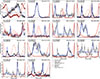 |
Fig. 1. Light curve fitting from the first sample of MSPs, with the black curve and the dark red curves corresponding to the γ-ray and radio data, respectively. The light blue and the orange curves correspond to the γ-ray light curves and radio profiles, respectively. Finally, the light blue dotted and orange dotted curves obtained from the same fitting, but imposing a perfect alignment, signifying ζ = i. |
4.1.1. J0218+4232
This pulsar of a period of P = 2.32 ms shows one wide γ-ray peak during almost the whole period, along with one radio peak with a complex shape, which could be due to a hollow cone geometry or possibly a characteristic of multipolar magnetic field components. The radio profile also presents a wide interpulse with a small amplitude. The light curve fit provides ![Mathematical equation: $ \chi = 66.6 [+0.4,-0.6]{\circ} $](/articles/aa/full_html/2026/03/aa56461-25/aa56461-25-eq16.gif) , ζ = 14.2[+1.7, −1.1]°, and ϕ = 0.095. Rather than one wide peak, the modelled light curve shows two unresolved γ-ray peaks. Indeed, this type of light curve with one very large peak is not aptly predicted by the model. However, the fitting is still accurate, with a p-value of 0.19. The predicted radio profile is also rather good, considering the complex shape of the radio pulse; however, we did miss the small interpulse. The fitted ζ angle is far from what has been obtained with Shapiro delay, with i = 85.2° (Tan et al. 2024). When a second fit imposing perfect alignment was carried out, the magnetic angle obtained was
, ζ = 14.2[+1.7, −1.1]°, and ϕ = 0.095. Rather than one wide peak, the modelled light curve shows two unresolved γ-ray peaks. Indeed, this type of light curve with one very large peak is not aptly predicted by the model. However, the fitting is still accurate, with a p-value of 0.19. The predicted radio profile is also rather good, considering the complex shape of the radio pulse; however, we did miss the small interpulse. The fitted ζ angle is far from what has been obtained with Shapiro delay, with i = 85.2° (Tan et al. 2024). When a second fit imposing perfect alignment was carried out, the magnetic angle obtained was ![Mathematical equation: $ \chi_i = 30.0 [+0.9,-0.1]{\circ} $](/articles/aa/full_html/2026/03/aa56461-25/aa56461-25-eq17.gif) , with a phase shift of ϕi = 0.035. We see that the curve deviates even further from the observed light curve, with a p-value of 0.0005. Indeed, we can see that the corresponding γ-ray light curve has two well-resolved pulses, which does not match at all the observed light curve. However, the radio pulse profile is rather accurate, showing both the pulse and the interpulse. With those results, we can conclude that this pulsar does not satisfy the hypothesis of alignment.
, with a phase shift of ϕi = 0.035. We see that the curve deviates even further from the observed light curve, with a p-value of 0.0005. Indeed, we can see that the corresponding γ-ray light curve has two well-resolved pulses, which does not match at all the observed light curve. However, the radio pulse profile is rather accurate, showing both the pulse and the interpulse. With those results, we can conclude that this pulsar does not satisfy the hypothesis of alignment.
4.1.2. J0437-4715
This pulsar of a period of P = 5.76 ms shows one γ-ray peak and one radio peak. The best-fit parameters for are ![Mathematical equation: $ \chi = 44.4 [+3.5,-12.8]{\circ} $](/articles/aa/full_html/2026/03/aa56461-25/aa56461-25-eq18.gif) , ζ = 44.0[+12.3, −3.5]° and ϕ = −0.04, with a p-value of 0.82. This is consistent with the orbital inclination angle deduced from Shapiro delay with i′ = 42.42°, assuming the complementary angle, i′=π − i, which gives the same γ-ray light curves due to symmetry considerations (Reardon et al. 2016). When a second fit imposing a perfect alignment was performed, we did indeed recover a very similar fitting, with a magnetic angle of
, ζ = 44.0[+12.3, −3.5]° and ϕ = −0.04, with a p-value of 0.82. This is consistent with the orbital inclination angle deduced from Shapiro delay with i′ = 42.42°, assuming the complementary angle, i′=π − i, which gives the same γ-ray light curves due to symmetry considerations (Reardon et al. 2016). When a second fit imposing a perfect alignment was performed, we did indeed recover a very similar fitting, with a magnetic angle of ![Mathematical equation: $ \chi_i = 44.5[+3.4,-0.5]{\circ} $](/articles/aa/full_html/2026/03/aa56461-25/aa56461-25-eq19.gif) and phase shift of ϕi = −0.035, as well as a slightly higher p-value of 0.91.
and phase shift of ϕi = −0.035, as well as a slightly higher p-value of 0.91.
4.1.3. J0737-3039A
This pulsar has the largest period of the sample, with P = 22.7 ms. It belongs to a very peculiar system, the only double pulsar system known so far. It shows two γ-ray peaks and a radio peak with interpulse, hinting for an almost perpendicular rotator. The fitting of the γ-ray light curve provides ![Mathematical equation: $ \chi = 63.7 [+26.1,-8.9]{\circ} $](/articles/aa/full_html/2026/03/aa56461-25/aa56461-25-eq20.gif) , ζ = 88.2[+1.8, −18.1]° and ϕ = 0.45. The separation of the two peaks being Δ = 0.506 ± 0.012, the large phase shift can be attributed to an inversion of the peaks. The fit is accurate, with a p-value of 0.93. This is coherent with the Shapiro delay, with i = 89.35° (Kramer et al. 2021). The resulting modelling of the radio pulse profile gives a radio interpulse with an amplitude and a shape that is not exactly the one obtained through observations, but it is fully centred on the observed peak, which is what we are looking for with this model. When a second fit imposing a perfect alignment was done, we were able to recover a very similar fitting, with a magnetic angle of
, ζ = 88.2[+1.8, −18.1]° and ϕ = 0.45. The separation of the two peaks being Δ = 0.506 ± 0.012, the large phase shift can be attributed to an inversion of the peaks. The fit is accurate, with a p-value of 0.93. This is coherent with the Shapiro delay, with i = 89.35° (Kramer et al. 2021). The resulting modelling of the radio pulse profile gives a radio interpulse with an amplitude and a shape that is not exactly the one obtained through observations, but it is fully centred on the observed peak, which is what we are looking for with this model. When a second fit imposing a perfect alignment was done, we were able to recover a very similar fitting, with a magnetic angle of ![Mathematical equation: $ \chi_i = 63.3 [+24.7,-6.8]{\circ} $](/articles/aa/full_html/2026/03/aa56461-25/aa56461-25-eq21.gif) , the same large phase shift ϕi = 0.45, and a p-value of 0.93.
, the same large phase shift ϕi = 0.45, and a p-value of 0.93.
4.1.4. J0740+6620
This pulsar of a period of P = 2.89 ms exhibits double γ-ray peaks and a radio peak with an interpulse. The results of the fit are ![Mathematical equation: $ \chi= 50.1 [+8.8,-7.1]{\circ} $](/articles/aa/full_html/2026/03/aa56461-25/aa56461-25-eq22.gif) , ζ = 83.4[+2.2, −3.2]°, and ϕ = −0.005. The fitting of the γ-ray light curve is accurate, with a p-value of 0.41. The modelled radio profile recovers the interpulse, however, with an amplitude that is too small. The fitted ζ angle is only a few degrees away from the inclination given by Shapiro delay, with i = 87.56° (Fonseca et al. 2021). For the second modelling, imposing a perfect alignment, we recovered a radio interpulse with a larger amplitude. The magnetic angle found is
, ζ = 83.4[+2.2, −3.2]°, and ϕ = −0.005. The fitting of the γ-ray light curve is accurate, with a p-value of 0.41. The modelled radio profile recovers the interpulse, however, with an amplitude that is too small. The fitted ζ angle is only a few degrees away from the inclination given by Shapiro delay, with i = 87.56° (Fonseca et al. 2021). For the second modelling, imposing a perfect alignment, we recovered a radio interpulse with a larger amplitude. The magnetic angle found is ![Mathematical equation: $ \chi_i = 38.8 [+2.9,-0.9]{\circ} $](/articles/aa/full_html/2026/03/aa56461-25/aa56461-25-eq23.gif) , with a phase shift ϕi = −0.005. The γ-ray light curve obtained is similar to the previous one, leading to a p-value of 0.16.
, with a phase shift ϕi = −0.005. The γ-ray light curve obtained is similar to the previous one, leading to a p-value of 0.16.
4.1.5. J0955-6150
This pulsar of a period of P = 1.99 ms is the fastest pulsar of the sample. It shows one strong and one weak γ-ray peak, as well as a radio peak with a complex shape. For this pulsar, the symmetrical solution has been taken. The fitting gives ![Mathematical equation: $ \chi = 32.6 [+10.5,-9.6]{\circ} $](/articles/aa/full_html/2026/03/aa56461-25/aa56461-25-eq24.gif) , ζ = 85.2[+1.7, −9.2]° and ϕ = −0.31. Due to the noise and the large delay between the two γ-ray peaks, the fitting was difficult to perform, as only the right part of the first γ-ray peak was recovered and the second γ-ray peak was too thin and the amplitude too small when compared to observations. Since the radio pulse is quite wide, it is hard to define the phase 0 of this profile. This uncertainty could explain the large phase shift obtained for this pulsar, better than a non-radial propagation effect in the γ-ray emission. The predicted radio profile shows a radio interpulse that is not observed, and overestimates the signal between the peaks. The fit is still accurate, with a p-value of 0.43. The best-fit ζ angle is consistent with Shapiro delay measurements, with i = 83.2° (Serylak et al. 2022). The two fits are very similar, with only the first γ-ray peak is a bit shifted to the left. The magnetic angle found for the fit imposing the Shapiro constraint is
, ζ = 85.2[+1.7, −9.2]° and ϕ = −0.31. Due to the noise and the large delay between the two γ-ray peaks, the fitting was difficult to perform, as only the right part of the first γ-ray peak was recovered and the second γ-ray peak was too thin and the amplitude too small when compared to observations. Since the radio pulse is quite wide, it is hard to define the phase 0 of this profile. This uncertainty could explain the large phase shift obtained for this pulsar, better than a non-radial propagation effect in the γ-ray emission. The predicted radio profile shows a radio interpulse that is not observed, and overestimates the signal between the peaks. The fit is still accurate, with a p-value of 0.43. The best-fit ζ angle is consistent with Shapiro delay measurements, with i = 83.2° (Serylak et al. 2022). The two fits are very similar, with only the first γ-ray peak is a bit shifted to the left. The magnetic angle found for the fit imposing the Shapiro constraint is ![Mathematical equation: $ \chi_i = 34.9[+15.9,-6.0]{\circ} $](/articles/aa/full_html/2026/03/aa56461-25/aa56461-25-eq25.gif) , the phase shift is the same as previously with ϕi = −0.31. The resulting p-value obtained is 0.51; thus, it is still accurate. The predicted radio pulse profile is slightly more accurate than the previous one, with a smaller interpulse.
, the phase shift is the same as previously with ϕi = −0.31. The resulting p-value obtained is 0.51; thus, it is still accurate. The predicted radio pulse profile is slightly more accurate than the previous one, with a smaller interpulse.
4.1.6. J1012-4235
This pulsar of a period of P = 3.1 ms shows a double peaked γ-ray profile and one radio peak. For this pulsar, the symmetrical solution has also been taken. The fitting of the γ-ray light curve gives ![Mathematical equation: $ \chi= 46.3 [+13.7,-4.2]{\circ} $](/articles/aa/full_html/2026/03/aa56461-25/aa56461-25-eq26.gif) , ζ = 89.4[+0.6, −2.0]°, and ϕ = 0.09. The fit is accurate, with a p-value of 0.58. The modelled radio pulse profile shows an interpulse that is not observed. The reason for this is given just below. The ζ angle obtained is compatible with the inclination given by Shapiro delay (Gautam et al. 2024), i = 87.97°. When a second fit imposing a perfect alignment was done, the γ-ray light curve was very similar to the previous one, but this time with a larger magnetic angle of
, ζ = 89.4[+0.6, −2.0]°, and ϕ = 0.09. The fit is accurate, with a p-value of 0.58. The modelled radio pulse profile shows an interpulse that is not observed. The reason for this is given just below. The ζ angle obtained is compatible with the inclination given by Shapiro delay (Gautam et al. 2024), i = 87.97°. When a second fit imposing a perfect alignment was done, the γ-ray light curve was very similar to the previous one, but this time with a larger magnetic angle of ![Mathematical equation: $ \chi_i = 85.0[+4.9,-10.7]{\circ} $](/articles/aa/full_html/2026/03/aa56461-25/aa56461-25-eq27.gif) . However, this does not impact the shape of the modelled light curve, due to symmetries in the γ-ray emission model. The phase shift is now also much larger, with ϕi = −0.41. The separation between the peaks could be larger than 0.5 considering the error bars, with Δ = 0.496 ± 0.008. Thus, obtaining a best fit that requires an inversion of the peaks is mathematically still possible; however, since there is no observed radio interpulse we do not have another way to define the beginning of the period and justify the inversion of the peaks (see Sect. 5 for more details). The p-value is now of 0.39. The radio pulse profile is slightly better than the previous one, still predicting an interpulse, but slightly smaller than before.
. However, this does not impact the shape of the modelled light curve, due to symmetries in the γ-ray emission model. The phase shift is now also much larger, with ϕi = −0.41. The separation between the peaks could be larger than 0.5 considering the error bars, with Δ = 0.496 ± 0.008. Thus, obtaining a best fit that requires an inversion of the peaks is mathematically still possible; however, since there is no observed radio interpulse we do not have another way to define the beginning of the period and justify the inversion of the peaks (see Sect. 5 for more details). The p-value is now of 0.39. The radio pulse profile is slightly better than the previous one, still predicting an interpulse, but slightly smaller than before.
The model assumes that the polar caps (from which the radio photons are emitted) are antipodal, but recent observations from the NICER mission (Gendreau et al. 2012) tend to show that this is not necessarily true. If this is the case, radio photons for an aligned rotator could be observed by looking at its equator or could miss an interpulse that should be observed for an orthogonal rotator. This effect is particularly important for MSPs, for which radio and γ-ray emission occurs close to the stellar surface. Since this feature is not taken into account in our model, this could explain the possible missing or false prediction of a non-existing interpulse in the radio profile resulting from an accurate γ-ray fit.
4.1.7. J1125-6014
This pulsar of a period of P = 2.63 ms shows weak double γ-ray peaks, and a radio peak with a weak interpulse. The number of data points for this pulsar being smaller than 30, using a KS test is less relevant. The fitting obtained seems rather good considering the noise in the data, even though the second γ-ray peak shows a complex structure possibly associated to a third peak, the fit focusses on the left part of the pulse. The predicted radio profile recovers the main pulse well, but misses the radio interpulses, probably for the same reason as that given for PSR J1012-4235. The best-fit parameters are ![Mathematical equation: $ \chi= 69.8 [+14.9,-47.2]{\circ} $](/articles/aa/full_html/2026/03/aa56461-25/aa56461-25-eq28.gif) , ζ = 44.1[+38.5, −15.8]° and ϕ = −0.06. The best-fit ζ angle is far from the value given by Shapiro delay, i = 77.6° (Shamohammadi et al. 2023), but given the error bars, we cannot exclude a possible alignment. When a second fit imposing a perfect alignment was done, we recovered a similar fitting: the first γ-ray peak is slightly thinner than the previous one and the second one now rather focusses on the right part of the possible double pulse. The magnetic angle obtained for this second fit is
, ζ = 44.1[+38.5, −15.8]° and ϕ = −0.06. The best-fit ζ angle is far from the value given by Shapiro delay, i = 77.6° (Shamohammadi et al. 2023), but given the error bars, we cannot exclude a possible alignment. When a second fit imposing a perfect alignment was done, we recovered a similar fitting: the first γ-ray peak is slightly thinner than the previous one and the second one now rather focusses on the right part of the possible double pulse. The magnetic angle obtained for this second fit is ![Mathematical equation: $ \chi_i = 42.7[+44.1,-13.4]{\circ} $](/articles/aa/full_html/2026/03/aa56461-25/aa56461-25-eq29.gif) and due to the shift of the second fitted peak, the phase shift is now much larger, with ϕi = −0.42. As it is also a faint pulsar with a low photon statistics, it is hard to draw a firm conclusion.
and due to the shift of the second fitted peak, the phase shift is now much larger, with ϕi = −0.42. As it is also a faint pulsar with a low photon statistics, it is hard to draw a firm conclusion.
4.1.8. J1600-3053
This pulsar of a period of P = 3.6 ms displays really close double γ-ray peaks and one radio peak. The results of the fit are ![Mathematical equation: $ \chi= 28.2 [+12.1,-3.8]{\circ} $](/articles/aa/full_html/2026/03/aa56461-25/aa56461-25-eq30.gif) , ζ = 67.7[+2.9, −11.0]°, and ϕ = −0.13. The fit is accurate, with a p-value of 0.75. The modelling of the radio profile is accurate, even though it slightly overestimates the signal between the peaks. The fitted ζ angle is very close to the measurement deduced from Shapiro delay, with i = 68.6° (Desvignes et al. 2016). Performing a second fit by imposing a perfect alignment, we recovered very similar fitting parameters, both in γ-rays and in radio, with a magnetic angle of
, ζ = 67.7[+2.9, −11.0]°, and ϕ = −0.13. The fit is accurate, with a p-value of 0.75. The modelling of the radio profile is accurate, even though it slightly overestimates the signal between the peaks. The fitted ζ angle is very close to the measurement deduced from Shapiro delay, with i = 68.6° (Desvignes et al. 2016). Performing a second fit by imposing a perfect alignment, we recovered very similar fitting parameters, both in γ-rays and in radio, with a magnetic angle of ![Mathematical equation: $ \chi_i = 25.7[+1.3,-0.7]{\circ} $](/articles/aa/full_html/2026/03/aa56461-25/aa56461-25-eq31.gif) , phase shift ϕi = −0.15, and p-value of 0.82.
, phase shift ϕi = −0.15, and p-value of 0.82.
4.1.9. J1614-2230
This pulsar of a period of P = 3.15 ms shows two main γ-ray peaks and one weak peak, as well as one radio peak with a weak interpulse. It is unclear if the weak γ-ray pulse should be associated to the strong peak or not. The results of the fitting are ![Mathematical equation: $ \chi= 41.8 [+0.2,-0.8]{\circ} $](/articles/aa/full_html/2026/03/aa56461-25/aa56461-25-eq32.gif) , ζ = 89.1[+0.5, −1.1]°, and ϕ = 0.005. The p-value is 0.02, smaller than the threshold fixed at 0.05 for a 5% confidence interval. This could come from the first γ-ray peak, which has an amplitude that is slightly too large compared to observations, while the second γ-ray peak has an amplitude that is a bit too small. Nevertheless, the p-value is still close from the threshold value and would be valid considering a criteria at 1% confidence level. The first radio peak is well recovered, but the modelled radio interpulse has a larger amplitude than what is observed. The Shapiro delay gives an inclination of i = 89.18° (Shamohammadi et al. 2023), which is consistent with what has been found for the fitted ζ angle. Thus, when a second fit imposing a perfect alignment was performed, we recovered a very similar fitting, with almost the same magnetic angle,
, ζ = 89.1[+0.5, −1.1]°, and ϕ = 0.005. The p-value is 0.02, smaller than the threshold fixed at 0.05 for a 5% confidence interval. This could come from the first γ-ray peak, which has an amplitude that is slightly too large compared to observations, while the second γ-ray peak has an amplitude that is a bit too small. Nevertheless, the p-value is still close from the threshold value and would be valid considering a criteria at 1% confidence level. The first radio peak is well recovered, but the modelled radio interpulse has a larger amplitude than what is observed. The Shapiro delay gives an inclination of i = 89.18° (Shamohammadi et al. 2023), which is consistent with what has been found for the fitted ζ angle. Thus, when a second fit imposing a perfect alignment was performed, we recovered a very similar fitting, with almost the same magnetic angle, ![Mathematical equation: $ \chi_i = 41.7[+0.3,-0.3]{\circ} $](/articles/aa/full_html/2026/03/aa56461-25/aa56461-25-eq33.gif) , phase shift ϕi = 0.005, and the same p-value of 0.02. This low p-value should be attributed to the fact that the third weak peak γ-ray peak was not reproduced by the model. Overall, it displays some similarities with PSR J1125-6014.
, phase shift ϕi = 0.005, and the same p-value of 0.02. This low p-value should be attributed to the fact that the third weak peak γ-ray peak was not reproduced by the model. Overall, it displays some similarities with PSR J1125-6014.
4.1.10. J1713+0747
This pulsar of a period of P = 4.57 ms shows one large γ-ray peak spread over a significant fraction of the period and one radio peak. As for PSR J0218+4232, this type of γ-ray light curve is not well reproduced by our model. The symmetrical solution has been kept, as for PSR J0955−6150 and PSR J1012−4235. The best-fit parameters are ![Mathematical equation: $ \chi= 26.7 [+2.3,-6.4]{\circ} $](/articles/aa/full_html/2026/03/aa56461-25/aa56461-25-eq34.gif) , ζ = 69.1[+0.7, −18.0]°, and ϕ = −0.05. The fitting is still accurate with a p-value of 0.64. The fitted ζ angle is only a few degrees away from what is given by Shapiro delay, with i = 72° (Fonseca et al. 2016). When a second fit imposing a perfect alignment was carried out, we obtained two unresolved γ-ray peaks rather than one wide peak. The magnetic angle found is
, ζ = 69.1[+0.7, −18.0]°, and ϕ = −0.05. The fitting is still accurate with a p-value of 0.64. The fitted ζ angle is only a few degrees away from what is given by Shapiro delay, with i = 72° (Fonseca et al. 2016). When a second fit imposing a perfect alignment was carried out, we obtained two unresolved γ-ray peaks rather than one wide peak. The magnetic angle found is ![Mathematical equation: $ \chi_i = 29.6[+0.4,-0.5]{\circ} $](/articles/aa/full_html/2026/03/aa56461-25/aa56461-25-eq35.gif) , with a phase shift of ϕi = −0.03 and the p-value is now 0.24. However, the radio pulse profile is very similar.
, with a phase shift of ϕi = −0.03 and the p-value is now 0.24. However, the radio pulse profile is very similar.
4.1.11. J1741+1351a
This pulsar of a period of P = 3.75 ms shows one weak and one strong γ-ray peak, as well as one radio peak with a weak interpulse. The fitting parameters are ![Mathematical equation: $ \chi= 39.8 [+13.0,-8.6]{\circ} $](/articles/aa/full_html/2026/03/aa56461-25/aa56461-25-eq36.gif) , ζ = 50.1[+8.6, −11.4]°, and ϕ = 0.31. The fit is accurate, with a p-value of 0.30, even if we completely miss the first γ-ray peak. Indeed, this peak is not statistically significant since it is mostly composed of one small amplitude data point. The large phase shift can also be attributed to the missing γ-ray peak. The modelled γ-ray light curve only reproduces one peak, but since the actual light curve shows two peaks, the predicted single peak light curve has to be shifted to later phases to fit the second observed peak. Concerning the radio profile, we miss the small interpulse. The inclination given by Shapiro delay slightly differs from the best-fit ζ angle, even considering the error bars, with i = 73° (Arzoumanian et al. 2018). When a second fit imposing a perfect alignment was done, we indeed recovered two peaks, but the second one remains slightly too thin compared to the observations. The magnetic angle found is
, ζ = 50.1[+8.6, −11.4]°, and ϕ = 0.31. The fit is accurate, with a p-value of 0.30, even if we completely miss the first γ-ray peak. Indeed, this peak is not statistically significant since it is mostly composed of one small amplitude data point. The large phase shift can also be attributed to the missing γ-ray peak. The modelled γ-ray light curve only reproduces one peak, but since the actual light curve shows two peaks, the predicted single peak light curve has to be shifted to later phases to fit the second observed peak. Concerning the radio profile, we miss the small interpulse. The inclination given by Shapiro delay slightly differs from the best-fit ζ angle, even considering the error bars, with i = 73° (Arzoumanian et al. 2018). When a second fit imposing a perfect alignment was done, we indeed recovered two peaks, but the second one remains slightly too thin compared to the observations. The magnetic angle found is ![Mathematical equation: $ \chi_i = 81.2[+0.8,-1.2]{\circ} $](/articles/aa/full_html/2026/03/aa56461-25/aa56461-25-eq37.gif) with a phase shift ϕi = 0.05 and the p-value becomes 0.44. The predicted radio profile shows a very small interpulse, not centred on the one observed. Even if both fits (general and imposing alignment) pass the KS test, physically, it is more accurate to find two γ-ray pulses, which favours the solution with the Shapiro constraint, so we do not have enough arguments to exclude the hypothesis of alignment for this pulsar.
with a phase shift ϕi = 0.05 and the p-value becomes 0.44. The predicted radio profile shows a very small interpulse, not centred on the one observed. Even if both fits (general and imposing alignment) pass the KS test, physically, it is more accurate to find two γ-ray pulses, which favours the solution with the Shapiro constraint, so we do not have enough arguments to exclude the hypothesis of alignment for this pulsar.
4.1.12. J1857+0943
This pulsar of a period of P = 5.36 ms shows a weak signal, made of double γ-ray peaks, and one radio peak with an interpulse. The number of data points for this pulsar is smaller than 30, making a KS test less relevant; also, the peak structure not particularly visible. Even if considering the noise in the data, the fit is overall reasonable, the first peak is poorly reproduced, its amplitude is very small, and it does not seem well centred. The second peak amplitude is a better, but it is too thin and not well centred. The predicted radio profile reproduces the main pulse well, but misses the interpulse. It gives ![Mathematical equation: $ \chi= 80.9 [+9.1,-52.6]{\circ} $](/articles/aa/full_html/2026/03/aa56461-25/aa56461-25-eq38.gif) , ζ = 63.8[+26.1, −35.8]° and ϕ = 0.50. Given the large uncertainties, it is hard to reach any conclusion concerning the large phase shift. The inclination given by Shapiro delay is i = 88.0° (Arzoumanian et al. 2018), which, considering the error bars, is in agreement with the value of the best-fit ζ angle. When a second fit imposing a perfect alignment was done, the γ-ray light curve obtained is slightly different from the one found previously. The first γ-ray peak obtained seems better centred on the observed one, but is thinner. This time we recover a small interpulse for the radio profile. The magnetic angle found for this second fit is
, ζ = 63.8[+26.1, −35.8]° and ϕ = 0.50. Given the large uncertainties, it is hard to reach any conclusion concerning the large phase shift. The inclination given by Shapiro delay is i = 88.0° (Arzoumanian et al. 2018), which, considering the error bars, is in agreement with the value of the best-fit ζ angle. When a second fit imposing a perfect alignment was done, the γ-ray light curve obtained is slightly different from the one found previously. The first γ-ray peak obtained seems better centred on the observed one, but is thinner. This time we recover a small interpulse for the radio profile. The magnetic angle found for this second fit is ![Mathematical equation: $ \chi_i = 62.5[+27.4,-16.4]{\circ} $](/articles/aa/full_html/2026/03/aa56461-25/aa56461-25-eq39.gif) and the phase shift is ϕi = 0.02. The statistics of this pulsar is certainly too poor to make any firm conclusion about the fitting results.
and the phase shift is ϕi = 0.02. The statistics of this pulsar is certainly too poor to make any firm conclusion about the fitting results.
4.1.13. J1909-3744
This pulsar of a period of P = 2.95 ms shows weak double γ-ray peaks and one radio peak. The number of data points for this pulsar is smaller than 30, making a KS test less relevant. However, the fitting of the γ-ray light curve seems accurate, even if it is hard to tell if the first γ-ray peak is well centred or not on the observed pulse. The modelling of the radio pulse profile shows an interpulse that is not observed, the reason is the same as for PSR J1012−4235 and PSR J1125−6014 for which we had the same problem. The best-fit parameters are ![Mathematical equation: $ \chi= 74.4 [+15.6,-30.9]{\circ} $](/articles/aa/full_html/2026/03/aa56461-25/aa56461-25-eq40.gif) , ζ = 86.1[+3.9, −46.6]°, and ϕ = −0.02. The fitted ζ angle is consistent with the Shapiro delay expectation, with i = 86.69° (Shamohammadi et al. 2023). When a second fit imposing a perfect alignment was done, the γ-ray light curve and radio pulse profile obtained are close to the previous ones, only the amplitude of the first γ-ray peak is slightly larger compared to the previous result. The magnetic angle found for this second fit is
, ζ = 86.1[+3.9, −46.6]°, and ϕ = −0.02. The fitted ζ angle is consistent with the Shapiro delay expectation, with i = 86.69° (Shamohammadi et al. 2023). When a second fit imposing a perfect alignment was done, the γ-ray light curve and radio pulse profile obtained are close to the previous ones, only the amplitude of the first γ-ray peak is slightly larger compared to the previous result. The magnetic angle found for this second fit is ![Mathematical equation: $ \chi_i = 69.0[+20.9,-23.7]{\circ} $](/articles/aa/full_html/2026/03/aa56461-25/aa56461-25-eq41.gif) , with a phase shift of ϕi = −0.02.
, with a phase shift of ϕi = −0.02.
4.1.14. J2043+1711
This pulsar of a period of P = 2.38 ms shows double γ-ray peaks and one radio peak. The fit gives ![Mathematical equation: $ \chi= 31.8 [+0.9,-0.4]{\circ} $](/articles/aa/full_html/2026/03/aa56461-25/aa56461-25-eq42.gif) , ζ = 82.2[+0.4, −0.2]°, and ϕ = 0.02. The fitting seems to be accurate; however, the p-value obtained is of 0.01, out of the 5% confidence interval but surprising since the fit seems to reproduce well the observations in the γ-rays. However, the modelled radio profile overestimates the signal between the peaks, and shows an interpulse that is not observed. As for PSR J1614−2230, the p-value is still close from the threshold value and would be valid considering a criteria at 1% confidence level. The fitted ζ angle is very close to the inclination found through Shapiro delay, with i = 83.2° (Fonseca et al. 2016). When a second fit imposing a perfect alignment was done, for the magnetic angle, we obtained
, ζ = 82.2[+0.4, −0.2]°, and ϕ = 0.02. The fitting seems to be accurate; however, the p-value obtained is of 0.01, out of the 5% confidence interval but surprising since the fit seems to reproduce well the observations in the γ-rays. However, the modelled radio profile overestimates the signal between the peaks, and shows an interpulse that is not observed. As for PSR J1614−2230, the p-value is still close from the threshold value and would be valid considering a criteria at 1% confidence level. The fitted ζ angle is very close to the inclination found through Shapiro delay, with i = 83.2° (Fonseca et al. 2016). When a second fit imposing a perfect alignment was done, for the magnetic angle, we obtained ![Mathematical equation: $ \chi_i = 32.7[+0.3,-0.3]{\circ} $](/articles/aa/full_html/2026/03/aa56461-25/aa56461-25-eq43.gif) , while for the phase shift, we obtained ϕi = 0.03. The result becomes more accurate, with a p-value of 0.13. The γ-ray light curve obtained is very similar to the previous one, as well as the radio profile.
, while for the phase shift, we obtained ϕi = 0.03. The result becomes more accurate, with a p-value of 0.13. The γ-ray light curve obtained is very similar to the previous one, as well as the radio profile.
4.2. Discussion
We summarise our findings from this first sample by showing the histograms of the best-fit parameters (χ,ζ,ϕ) in Fig. 2, in the form of cosine distributions for angles χ and ζ. Considering the unconstrained fits, the distribution of cos ζ is bimodal, with one peak close to cos90 ° = 0, whose origin lies in the selection bias of our MSP sample. Indeed, one important criteria for their selection was to look for existing Shapiro delay measurements to determine the orbital inclination angle i. This Shapiro effect is particularly strong for edge-on binaries, meaning i ≈ 90°, which explains the observed distribution for cos ζ. This bias is even more pronounced for the distribution of cos i angles. However, there is also a second peak around cos ζ = cos40 ° ≈0.8, which is mostly due to the non-aligned pulsars of our sample. The distribution of cos χ for the same unconstrained fits peaks at values close to cos40 ° ≈0.8, although the statistic is low. The distribution for the constrained fit imposing i = ζ follows the same trend closely. However, the sample of MSPs we considered is rather small, so those claims should be taken with caution. Considering the distribution of the phase shift ϕ, it peaks at a mean value of 0.06 and has a median of 0.0; however, we can see that a non negligible part of the pulsars from the sample present a large phase shift. A more detailed discussion about this observation is presented in Sect. 5, including pulsars from the second sample.
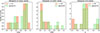 |
Fig. 2. Histogram of the best-fit parameters cos χ (left), cos ζ (middle), and ϕ (right) for the first sample of MSPs, in green in the general case and in orange for the fitting imposing i = ζ. |
Figure 3 gives a summary of the best-fit parameters, on the left, in the χ−ζ plane showing the couple χ and ζ, and on the right, in the ζ − i plane. Giving the timescale of alignment during the accretion phase of the binary, we would expect those two angles to be equal, as it is represented by the blue dotted line. The majority of the pulsars are well aligned on the ζ = i line: only one of them, PSR J0218+4232, is completely misaligned, while three of them are only a few degrees away from an alignment (between 1° and 3°): PSR J0740+6620, PSR J1713+0747, PSR J2043+1711. In the end, 71% of them are shown to be perfectly aligned and we reached a level of 93% for the alignment by including those only a few degrees away from perfect alignment. A possible explanation for the misalignment of PSR J0218+4232 could be a movement of precession induced by additional torques acting during the accretion phase, not taken into account by the current model or simply a too long alignment timescale. However, the shape of its light curve is not well explained by the model used and, thus, the quality of the fit can still be questioned.
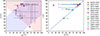 |
Fig. 3. Left: χ−ζ plane showing the best-fit couple of angles χ and ζ for the first sample of MSPs. Right: ζ − i plane showing the best-fit angle, ζ, for the inclination, i, imposed by Shapiro delay measurements, with the blue dotted line corresponding to the perfect alignment condition i = ζ. Individual pulsars are depicted by different colours. |
To verify whether the 93% of aligned pulsars could have been obtained by chance, we performed a reduced  test for the ratio between the viewing angle, ζ, and inclination angle, i, following the idea of Laycock et al. (2025). The quantity to test is R = ζ/i, which in theory is equal to one, according to our understanding of the evolution of a pulsar in a binary. The associated reduced
  is defined by
 (4)
(4)
with n being the number of pulsars in our sample (here n = 14), d the number of degrees of freedom (d = n − 1), and σk the error on the ratio R, obtained from the propagation of the errors made on the estimation of ζ. Its value must be compared to a critical value associated to a probability to find by chance a result above this critical value. The latter is found in a  table, and for a confidence level of 99.9% (meaning having a probability of 0.001 to find a higher value), the critical value is
  . However, the value for our sample is
  , far above the critical value, and thus excluding the possibility that this result has been obtained by chance.
4.3. Second sample
The second sample of MSPs is based on Blanchard et al. (2025), who studied the phenomenon of eclipses in spider binary pulsars. For the sample they considered, they provide the different inclination angle measurements available in the literature. Those are summarised in Table 2. The idea is to use the same algorithm as previously to fit the γ-ray light curves of this new sample of MSPs, in order to left the degeneracy between those results. The fitting was done a first time without any constraints on the viewing angle, ζ, and then a second time with a restriction of the possible values of this angle on the interval given by the literature in Table 2. The different fits obtained are shown on Figure 4, using the same legend as in Fig. 1. The quality of the fits is discussed in the following paragraphs.
4.3.1. J0023+0923
This pulsar of a period of P = 3.05 ms (Breton et al. 2013; Draghis et al. 2019; Mata Sánchez et al. 2023) shows two unresolved γ-ray peaks and one complex radio peak with three components. The parameters of the fit are ![Mathematical equation: $ \chi = 27.0 [+11.5,-3.1]{\circ} $](/articles/aa/full_html/2026/03/aa56461-25/aa56461-25-eq50.gif) , ζ = 70.1[+2.9, −10.1]°, and ϕ = 0.01. The γ-ray fit is accurate, with a p-value of 0.93. The predicted radio profile does not reproduce in details the complex structure of the radio peak, but once again this is not what we are looking at. For the second fit made on the interval for the inclination given in Blanchard et al. (2025), the best-fit angles are
, ζ = 70.1[+2.9, −10.1]°, and ϕ = 0.01. The γ-ray fit is accurate, with a p-value of 0.93. The predicted radio profile does not reproduce in details the complex structure of the radio peak, but once again this is not what we are looking at. For the second fit made on the interval for the inclination given in Blanchard et al. (2025), the best-fit angles are ![Mathematical equation: $ \chi_i = 27.2 [+31.2,-3.6]{\circ} $](/articles/aa/full_html/2026/03/aa56461-25/aa56461-25-eq51.gif) , i = 70.0[+2.9, −28.8]°, and ϕi = 0.03. The value of the inclination is compatible with the hypothesis of alignment. This second γ-ray fit is still accurate, with a p-value of 0.85, and it is very similar to the previous one, both in γ-ray and in radio.
, i = 70.0[+2.9, −28.8]°, and ϕi = 0.03. The value of the inclination is compatible with the hypothesis of alignment. This second γ-ray fit is still accurate, with a p-value of 0.85, and it is very similar to the previous one, both in γ-ray and in radio.
4.3.2. J0101-6422
This pulsar of a period of P = 2.57 ms shows one strong peak and one weak interpulse in the radio and double peaks in the γ-ray domain. For this pulsar, the symmetrical solution has been taken. The γ-ray light curve and radio pulse profile are rather well fitted, even though the amplitude of the first modelled γ-ray peak is small compared to observations. The result is ![Mathematical equation: $ \chi = 26.6 [+1.1,-0.6]{\circ} $](/articles/aa/full_html/2026/03/aa56461-25/aa56461-25-eq52.gif) , ζ = 75.4[+0.6, −0.4]° and ϕ = 0.495 for the best fit. The separation of the two peaks is smaller than 0.5 considering the maximum of the peaks; however, the second predicted γ-ray peak is not centred on a maximum but is shifted to the right, leading to a separation of the predicted peaks larger than 0.5. Thus the large phase shift can still be attributed to an inversion of the peaks. The fit is not accurate, with a p-value of 0.01. This might come from the second peak that is too thin compared to what is observed, but the p-value is still close from the threshold value and would be valid considering a criteria at 1% confidence level. However, the modelled radio profile does not recover the weak interpulse, probably for the same reason as for other pulsars in the previous sample (PSR J1012−4235, PSR J1125−6014 and PSR J1909−3744). When a second fit on the interval given by Shamohammadi et al. (2023) was done, the results were:
, ζ = 75.4[+0.6, −0.4]° and ϕ = 0.495 for the best fit. The separation of the two peaks is smaller than 0.5 considering the maximum of the peaks; however, the second predicted γ-ray peak is not centred on a maximum but is shifted to the right, leading to a separation of the predicted peaks larger than 0.5. Thus the large phase shift can still be attributed to an inversion of the peaks. The fit is not accurate, with a p-value of 0.01. This might come from the second peak that is too thin compared to what is observed, but the p-value is still close from the threshold value and would be valid considering a criteria at 1% confidence level. However, the modelled radio profile does not recover the weak interpulse, probably for the same reason as for other pulsars in the previous sample (PSR J1012−4235, PSR J1125−6014 and PSR J1909−3744). When a second fit on the interval given by Shamohammadi et al. (2023) was done, the results were: ![Mathematical equation: $ \chi_i = 28.4 [+1.6,-1.4]{\circ} $](/articles/aa/full_html/2026/03/aa56461-25/aa56461-25-eq53.gif) , i = 74.5[+0.5, −1.1]°, and ϕi = 0.495. The value of the inclination found is consistent with the best-fit ζ angle. Indeed, we recovered a very similar result for the γ-ray and radio profiles; as for the previous fit, the p-value is too small (0.002) compared to our criteria 0.002.
, i = 74.5[+0.5, −1.1]°, and ϕi = 0.495. The value of the inclination found is consistent with the best-fit ζ angle. Indeed, we recovered a very similar result for the γ-ray and radio profiles; as for the previous fit, the p-value is too small (0.002) compared to our criteria 0.002.
4.3.3. J0610-2100
This pulsar of a period of P = 3.86 ms (van der Wateren et al. 2022) shows two wide γ-ray peaks and one radio peak with a weak interpulse. The best-fit parameters are ![Mathematical equation: $ \chi = 43.5 [+14.5,-18.3]{\circ} $](/articles/aa/full_html/2026/03/aa56461-25/aa56461-25-eq54.gif) , ζ = 51.3[+17.4, −13.3]°, and ϕ = −0.25. Considering the uncertainties in the data, the modelled γ-ray light curve fits rather well the second peak, but misses completely the first peak. Due to those large uncertainties in the data, we cannot draw any firm conclusion concerning the large phase shift. However, according to the KS test it is still accurate, with a p-value of 0.22. Another solution that would be able to model both pulses is also possible, but it is not the one favoured by our method. Concerning the radio profile, the main pulse is rather well fitted, but we did not recover the interpulse (for the same reason as given for the cases described above). The fitting using the constraint on the inclination from Blanchard et al. (2025) yields a similar fitting for the γ-ray curve, with
, ζ = 51.3[+17.4, −13.3]°, and ϕ = −0.25. Considering the uncertainties in the data, the modelled γ-ray light curve fits rather well the second peak, but misses completely the first peak. Due to those large uncertainties in the data, we cannot draw any firm conclusion concerning the large phase shift. However, according to the KS test it is still accurate, with a p-value of 0.22. Another solution that would be able to model both pulses is also possible, but it is not the one favoured by our method. Concerning the radio profile, the main pulse is rather well fitted, but we did not recover the interpulse (for the same reason as given for the cases described above). The fitting using the constraint on the inclination from Blanchard et al. (2025) yields a similar fitting for the γ-ray curve, with ![Mathematical equation: $ \chi_i = 34.3 [+7.7,-9.3]{\circ} $](/articles/aa/full_html/2026/03/aa56461-25/aa56461-25-eq55.gif) , i = 60.6[+8.8, −6.6]°, and ϕi = 0.27. The p-value is also of 0.22. The light curve is slightly shifted to the right compared to previous fit, while the main radio pulse is wider. The best-fit angles i and ζ are compatible, so we can conclude that there is indeed an alignment for this pulsar.
, i = 60.6[+8.8, −6.6]°, and ϕi = 0.27. The p-value is also of 0.22. The light curve is slightly shifted to the right compared to previous fit, while the main radio pulse is wider. The best-fit angles i and ζ are compatible, so we can conclude that there is indeed an alignment for this pulsar.
4.3.4. J0636+5128
This pulsar of a period of P = 2.87 ms (Kaplan et al. 2018) shows two γ-ray peaks and one strong radio pulse. There are not enough date points for this γ-ray light curve to perform a KS test, but by eye, we can already see that the fit does not recover the first γ-ray peak. Indeed the error bars are not restrictive enough to be able to detect the first peak with our method. Concerning the radio pulse profile, the pulse seems accurately recovered. The results of the fit are ![Mathematical equation: $ \chi = 43.3 [+45.0,-25.7]{\circ} $](/articles/aa/full_html/2026/03/aa56461-25/aa56461-25-eq56.gif) , ζ = 47.9[+33.6, −28.8]°, and ϕ = 0.46. As for PSR J0610−2100, the uncertainties are too large to draw any conclusion on the large phase shift. The fitting imposing the constraint on the inclination from Blanchard et al. (2025) yields a very similar result, with
, ζ = 47.9[+33.6, −28.8]°, and ϕ = 0.46. As for PSR J0610−2100, the uncertainties are too large to draw any conclusion on the large phase shift. The fitting imposing the constraint on the inclination from Blanchard et al. (2025) yields a very similar result, with ![Mathematical equation: $ \chi_i = 59.9 [+15.0,-7.3]{\circ} $](/articles/aa/full_html/2026/03/aa56461-25/aa56461-25-eq57.gif) , i = 25.7[+2.2, −4.7]°, and ϕi = 0.46. Due to too few points in the γ-ray light curve and the large error bars associated to them, the fitting does not add real constraints on top of the geometrical constraints imposed for the observation in the γ-ray and radio domains; thus, the best-fit ζ is compatible with the value of the inclination we found.
, i = 25.7[+2.2, −4.7]°, and ϕi = 0.46. Due to too few points in the γ-ray light curve and the large error bars associated to them, the fitting does not add real constraints on top of the geometrical constraints imposed for the observation in the γ-ray and radio domains; thus, the best-fit ζ is compatible with the value of the inclination we found.
4.3.5. J1124-3653
This pulsar of a period of P = 2.41 ms shows two γ-ray peaks that are almost unresolved and one wide radio peak with a large interpulse. The best-fit parameters obtained are ![Mathematical equation: $ \chi = 53.5 [+4.2,-4.4]{\circ} $](/articles/aa/full_html/2026/03/aa56461-25/aa56461-25-eq58.gif) , ζ = 36.6[+7.3, −3.6]°, and ϕ = −0.025. The fitting of the γ-ray light curve is accurate, with a p-value of 0.13. The fit shows two unresolved γ-ray peaks that fit rather well the first peak, but we missed the second peak. The modelled radio pulse profile is rather good considering the noise, but we missed the interpulse. When the constraint on the inclination from Blanchard et al. (2025) was imposed, the result was similar, with
, ζ = 36.6[+7.3, −3.6]°, and ϕ = −0.025. The fitting of the γ-ray light curve is accurate, with a p-value of 0.13. The fit shows two unresolved γ-ray peaks that fit rather well the first peak, but we missed the second peak. The modelled radio pulse profile is rather good considering the noise, but we missed the interpulse. When the constraint on the inclination from Blanchard et al. (2025) was imposed, the result was similar, with ![Mathematical equation: $ \chi_i = 50.4 [+0.6,-2.3]{\circ} $](/articles/aa/full_html/2026/03/aa56461-25/aa56461-25-eq59.gif) , i = 44.5[+1.2, −0.5]°, and ϕi = −0.015. The p-value here is 0.09. No second γ-ray peak was predicted, as well as no radio interpulse, as in the case of the previous fit. The inclination angle found is compatible with the hypothesis of alignment.
, i = 44.5[+1.2, −0.5]°, and ϕi = −0.015. The p-value here is 0.09. No second γ-ray peak was predicted, as well as no radio interpulse, as in the case of the previous fit. The inclination angle found is compatible with the hypothesis of alignment.
4.3.6. J1514-4946
This pulsar of a period of P = 3.59 ms shows close double γ-ray peaks and one radio peak. For this pulsar, the symmetrical solution has been kept. The fitting of the curves provides ![Mathematical equation: $ \chi= 27.8 [+0.2,-0.5]{\circ} $](/articles/aa/full_html/2026/03/aa56461-25/aa56461-25-eq60.gif) , ζ = 74.2[+0.5, −0.2]°, and ϕ = 0.015. The fit looks rather accurate; however, according to the KS test the p-value is only of 0.0006. This could come from the amplitude of the modelled peak that is too small compared to what is observed. The radio pulse obtained is slightly too large. When a second fit imposing the constraint on the inclination from Shamohammadi et al. (2023) was done, the γ-ray light curve obtained corresponds actually exactly to the previous one, with
, ζ = 74.2[+0.5, −0.2]°, and ϕ = 0.015. The fit looks rather accurate; however, according to the KS test the p-value is only of 0.0006. This could come from the amplitude of the modelled peak that is too small compared to what is observed. The radio pulse obtained is slightly too large. When a second fit imposing the constraint on the inclination from Shamohammadi et al. (2023) was done, the γ-ray light curve obtained corresponds actually exactly to the previous one, with ![Mathematical equation: $ \chi_i = 27.8 [+0.2,-0.5]{\circ} $](/articles/aa/full_html/2026/03/aa56461-25/aa56461-25-eq61.gif) , i = 74.2[+0.5, −0.2]°, and ϕi = 0.015, as well as the same p-value of 0.0006. The radio profile is also the same as before. Thus, this pulsar respects the hypothesis of alignment.
, i = 74.2[+0.5, −0.2]°, and ϕi = 0.015, as well as the same p-value of 0.0006. The radio profile is also the same as before. Thus, this pulsar respects the hypothesis of alignment.
4.3.7. J1544+4937
This pulsar of a period of P = 2.16 ms (Mata Sánchez et al. 2023) shows one wide γ-ray peak spread out over almost the whole period and one radio peak. There are too few points to perform the KS test, but by eye, we can see that the γ-ray fit seems accurate. The predicted radio profile is also acceptable. The best-fit parameters are ![Mathematical equation: $ \chi = 60.5 [+6.4,-25.6]{\circ} $](/articles/aa/full_html/2026/03/aa56461-25/aa56461-25-eq62.gif) , ζ = 25.5[+24.0, −9.5]°, and ϕ = −0.02. The fitting using the constraint given by Blanchard et al. (2025) yields a similar fitting for the γ-ray light curve, with a peak that is thinner but of similar amplitude. The radio pulse is also thinner than previously. The best-fit parameters are
, ζ = 25.5[+24.0, −9.5]°, and ϕ = −0.02. The fitting using the constraint given by Blanchard et al. (2025) yields a similar fitting for the γ-ray light curve, with a peak that is thinner but of similar amplitude. The radio pulse is also thinner than previously. The best-fit parameters are ![Mathematical equation: $ \chi_i = 44.1 [+9.0,-17.4]{\circ} $](/articles/aa/full_html/2026/03/aa56461-25/aa56461-25-eq63.gif) , i = 48.3[+5.6, −5.3]°, and ϕi = 0.02. Considering the large error bars on the best-fit ζ, the inclination found is still compatible with an alignment.
, i = 48.3[+5.6, −5.3]°, and ϕi = 0.02. Considering the large error bars on the best-fit ζ, the inclination found is still compatible with an alignment.
4.3.8. J1555-2908
This pulsar of a period of P = 1.79 ms (Clark et al. 2023) shows two γ-ray peaks, a main peak with a large amplitude and a second smaller one, and one large radio peak with an interpulse. The best-fit parameters are ![Mathematical equation: $ \chi = 67.4 [+4.2,-27.3]{\circ} $](/articles/aa/full_html/2026/03/aa56461-25/aa56461-25-eq64.gif) , ζ = 70.7[+12.7, −3.7]°, and ϕ = 0.37. The separation of the two peaks being Δ = 0.554 ± 0.007, the large phase shift can be attributed to an inversion of the peaks. The fitting of the γ-ray light curve is accurate, with a p-value of 0.82. The modelled radio profile recovers well the main radio pulse but does not predict the interpulse, probably due to the limitation of our model. The fit that imposes a constraint on the inclination from Blanchard et al. (2025) yields a very similar fit both in radio and in γ-rays, with
, ζ = 70.7[+12.7, −3.7]°, and ϕ = 0.37. The separation of the two peaks being Δ = 0.554 ± 0.007, the large phase shift can be attributed to an inversion of the peaks. The fitting of the γ-ray light curve is accurate, with a p-value of 0.82. The modelled radio profile recovers well the main radio pulse but does not predict the interpulse, probably due to the limitation of our model. The fit that imposes a constraint on the inclination from Blanchard et al. (2025) yields a very similar fit both in radio and in γ-rays, with ![Mathematical equation: $ \chi_i = 58.5 [+6.4,-22.4]{\circ} $](/articles/aa/full_html/2026/03/aa56461-25/aa56461-25-eq65.gif) , i = 76.8[+7.9, −1.8]°, and ϕi = 0.37, which is compatible with the hypothesis of alignment. The p-value is of 0.82 here as well.
, i = 76.8[+7.9, −1.8]°, and ϕi = 0.37, which is compatible with the hypothesis of alignment. The p-value is of 0.82 here as well.
4.3.9. J1628-3205
This pulsar of a period of P = 3.21 ms (Li et al. 2014; Clark et al. 2023) shows two wide γ-ray peaks spread out on the whole period and one large radio pulse. The modelled γ-ray curve accurately fits the observed one, even though the amplitude of the first modelled peak is weak. The modelling of the radio pulse profile is rather good, even if the pulse is too wide. The best-fit parameters are ![Mathematical equation: $ \chi = 70.1 [+0.8,-2.1]{\circ} $](/articles/aa/full_html/2026/03/aa56461-25/aa56461-25-eq66.gif) , ζ = 22.7[+1.2, −2.1]°, and ϕ = −0.01, with a p-value of 0.43. The fit imposing the constraint on the inclination from Blanchard et al. (2025) yields an accurate γ-ray fit; however, only the first γ-ray peak is modelled. The predicted radio pulse is now thinner than previously. The results for this fit are
, ζ = 22.7[+1.2, −2.1]°, and ϕ = −0.01, with a p-value of 0.43. The fit imposing the constraint on the inclination from Blanchard et al. (2025) yields an accurate γ-ray fit; however, only the first γ-ray peak is modelled. The predicted radio pulse is now thinner than previously. The results for this fit are ![Mathematical equation: $ \chi_i = 29.3 [+9.7,-9.3]{\circ} $](/articles/aa/full_html/2026/03/aa56461-25/aa56461-25-eq67.gif) , i = 62.6[+7.4, −7.5]° and ϕi = −0.15, with a p-value of 0.19. The inclination is not compatible with the best-fit ζ angle, meaning that this pulsar does not respect the hypothesis of alignment. We tried to look at the symmetrical solution, which gave a very similar result to the one obtained imposing the Shapiro constraint, with one γ-ray pulse missing. Since having two γ-ray peaks is physically more accurate, this observation favours the first fit without the Shapiro constraint.
, i = 62.6[+7.4, −7.5]° and ϕi = −0.15, with a p-value of 0.19. The inclination is not compatible with the best-fit ζ angle, meaning that this pulsar does not respect the hypothesis of alignment. We tried to look at the symmetrical solution, which gave a very similar result to the one obtained imposing the Shapiro constraint, with one γ-ray pulse missing. Since having two γ-ray peaks is physically more accurate, this observation favours the first fit without the Shapiro constraint.
4.3.10. J1640+2224
This pulsar of a period of P = 3.16 ms shows close double γ-ray peaks and one radio peak. The results of the fitting are ![Mathematical equation: $ \chi= 62.1 [+2.9,-30.8]{\circ} $](/articles/aa/full_html/2026/03/aa56461-25/aa56461-25-eq68.gif) , ζ = 34.7[+30.1, −6.1]°, and ϕ = −0.03. The fit is accurate, with a p-value of 0.82, even though the amplitude of the second γ-ray peak is not well recovered. The fit imposing the constrain of the Shapiro measurements (Löhmer et al. 2005; Vigeland & Vallisneri 2014; Fonseca et al. 2016) yields
, ζ = 34.7[+30.1, −6.1]°, and ϕ = −0.03. The fit is accurate, with a p-value of 0.82, even though the amplitude of the second γ-ray peak is not well recovered. The fit imposing the constrain of the Shapiro measurements (Löhmer et al. 2005; Vigeland & Vallisneri 2014; Fonseca et al. 2016) yields ![Mathematical equation: $ \chi_i = 79.4 [+1.4,-5.2]{\circ} $](/articles/aa/full_html/2026/03/aa56461-25/aa56461-25-eq69.gif) , i = 71.0[+16.9, −17.0]°, and ϕi = −0.17. However, looking at the distribution obtained for the inclination, we notice that our method gives no strong constraint on the possible value for the inclination for the interval given in the literature. For this fit, we obtain two well-resolved peaks, which as seen by eye, does not correspond at all to the observed light curve. But due to the large error bars in the Fermi data, the fit is still considered as accurate, with a p-value of 0.16. The modelled radio profile is also less accurate than previously, the main peak being slightly too thin and a small interpulse that is not observed is predicted. Considering the error bars on the value of the best-fit ζ angle, this pulsar is aligned according to the measurements of Fonseca et al. (2016) (i = 60 ± 6°), but not aligned according to the results of Löhmer et al. (2005), Vigeland & Vallisneri (2014) (i = 84[+4, −6]°). Thus our solution favours the result of Fonseca et al. (2016), but we cannot reach a definitive conclusion on whether or not this pulsar is aligned.
, i = 71.0[+16.9, −17.0]°, and ϕi = −0.17. However, looking at the distribution obtained for the inclination, we notice that our method gives no strong constraint on the possible value for the inclination for the interval given in the literature. For this fit, we obtain two well-resolved peaks, which as seen by eye, does not correspond at all to the observed light curve. But due to the large error bars in the Fermi data, the fit is still considered as accurate, with a p-value of 0.16. The modelled radio profile is also less accurate than previously, the main peak being slightly too thin and a small interpulse that is not observed is predicted. Considering the error bars on the value of the best-fit ζ angle, this pulsar is aligned according to the measurements of Fonseca et al. (2016) (i = 60 ± 6°), but not aligned according to the results of Löhmer et al. (2005), Vigeland & Vallisneri (2014) (i = 84[+4, −6]°). Thus our solution favours the result of Fonseca et al. (2016), but we cannot reach a definitive conclusion on whether or not this pulsar is aligned.
4.3.11. J1732-5049
This pulsar of a period of P = 5.31 ms shows one wide γ-ray peak spread over a significant fraction of the period and one radio peak. The results of the fitting are ![Mathematical equation: $ \chi= 33.1 [+19.0,-6.7]{\circ} $](/articles/aa/full_html/2026/03/aa56461-25/aa56461-25-eq70.gif) , ζ = 62.9[+6.1, −17.6]°, and ϕ = 0.05. The fitted light curve shows two unresolved γ-ray peaks rather than one large peak, but the fitting is still considered as accurate with a p-value of 0.53. When the second fit imposing the constrain on the inclination from Shamohammadi et al. (2023) was done, we obtained a very similar results with
, ζ = 62.9[+6.1, −17.6]°, and ϕ = 0.05. The fitted light curve shows two unresolved γ-ray peaks rather than one large peak, but the fitting is still considered as accurate with a p-value of 0.53. When the second fit imposing the constrain on the inclination from Shamohammadi et al. (2023) was done, we obtained a very similar results with ![Mathematical equation: $ \chi_i = 32.4 [+5.4,-6.0]{\circ} $](/articles/aa/full_html/2026/03/aa56461-25/aa56461-25-eq71.gif) , i = 63.5[+5.3, −4.5]°, and ϕi = 0.05, compatible with the hypothesis of alignment. The p-value is the same as before, 0.53. The modelled radio profile is very similar in both cases as well. However it does not reproduce the complex shape of the radio pulse, as it was not the focus of this fitting.
, i = 63.5[+5.3, −4.5]°, and ϕi = 0.05, compatible with the hypothesis of alignment. The p-value is the same as before, 0.53. The modelled radio profile is very similar in both cases as well. However it does not reproduce the complex shape of the radio pulse, as it was not the focus of this fitting.
4.3.12. J1811-2405
This pulsar of a period of P = 2.7 ms shows one weak and one stronger γ-ray peak, as well as a radio peak with a weak interpulse. The results of the fitting are ![Mathematical equation: $ \chi= 34.7 [+21,-6.7]{\circ} $](/articles/aa/full_html/2026/03/aa56461-25/aa56461-25-eq72.gif) , ζ = 77.8[+3.2, −10.4]°, and ϕ = −0.1. The fit is accurate, with a p-value of 0.19. The amplitude of the second peak is rather small compared to what is observed, but the first peak is well recovered. The predicted radio profile seems also accurate, as we recovered the interpulse even though its amplitude is small. The results of the fit imposing using Shapiro delay from Ng et al. (2020) are
, ζ = 77.8[+3.2, −10.4]°, and ϕ = −0.1. The fit is accurate, with a p-value of 0.19. The amplitude of the second peak is rather small compared to what is observed, but the first peak is well recovered. The predicted radio profile seems also accurate, as we recovered the interpulse even though its amplitude is small. The results of the fit imposing using Shapiro delay from Ng et al. (2020) are ![Mathematical equation: $ \chi_i = 31.5[+5.4,-6.9]{\circ} $](/articles/aa/full_html/2026/03/aa56461-25/aa56461-25-eq73.gif) , i = 75.6[+3.4, −2.6]°, and ϕi = −0.07. This is consistent with the best-fit ζ angle obtained. We obtained a very similar result both in radio and in γ, with only the first γ-ray peak shifted to the right compared to what has been found previously. The corresponding p-value is 0.43.
, i = 75.6[+3.4, −2.6]°, and ϕi = −0.07. This is consistent with the best-fit ζ angle obtained. We obtained a very similar result both in radio and in γ, with only the first γ-ray peak shifted to the right compared to what has been found previously. The corresponding p-value is 0.43.
4.3.13. J1959+2048
This pulsar of a period of P = 1.61 ms shows one main thin γ-ray peak, as well as a second wider γ-ray pulse with a smaller amplitude. It also presents a complex radio pulse profile with three pulses: two strong ones separated by slightly less than half a period and one small interpulse close to one of the strong pulse. The results of the fit are ![Mathematical equation: $ \chi = 32.1 [+15.7,-4.2]{\circ} $](/articles/aa/full_html/2026/03/aa56461-25/aa56461-25-eq74.gif) , ζ = 85.2[+1.7, −4.9]°, and ϕ = 0.325. The separation of the two peaks being Δ = 0.566 ± 0.007, the large phase shift can be attributed to an inversion of the peaks. Another interpretation would be to identify the second radio pulse as the main pulse for phase-aligning the gamma rays. In this case, the radio peak at phase φ ≈ 0.3 would genuinely be the one at phase φ ≈ 0. The fit is accurate, with a p-value of 0.41. The second γ-ray peak is rather thin compared to the observed one, but it is well centred on it. The predicted radio profile is rather accurate: the main radio peak is a wide but well-centred; however, the interpulse has a complex shape composed of several peaks that are not all recovered, since only one interpulse can be predicted by the model. The fit using Shapiro delay constraints from Blanchard et al. (2025) deviates somehow from the previous fit, with
, ζ = 85.2[+1.7, −4.9]°, and ϕ = 0.325. The separation of the two peaks being Δ = 0.566 ± 0.007, the large phase shift can be attributed to an inversion of the peaks. Another interpretation would be to identify the second radio pulse as the main pulse for phase-aligning the gamma rays. In this case, the radio peak at phase φ ≈ 0.3 would genuinely be the one at phase φ ≈ 0. The fit is accurate, with a p-value of 0.41. The second γ-ray peak is rather thin compared to the observed one, but it is well centred on it. The predicted radio profile is rather accurate: the main radio peak is a wide but well-centred; however, the interpulse has a complex shape composed of several peaks that are not all recovered, since only one interpulse can be predicted by the model. The fit using Shapiro delay constraints from Blanchard et al. (2025) deviates somehow from the previous fit, with ![Mathematical equation: $ \chi_i = 69.5 [+2.4,-0.5]{\circ} $](/articles/aa/full_html/2026/03/aa56461-25/aa56461-25-eq75.gif) , i = 66.5[+0.5, −0.8]°, and ϕi = 0.325, with a p-value of 0.16. The γ-ray light curve obtained is similar to the previous one, only with peaks having a larger amplitude, but the inclination obtained is not compatible with the best-fit ζ angle. The only strong difference between the two fits is that in the case where ζ is left as a free parameter, the predicted radio profile is able to model the interpulse. This is not the case for the second fit using the Shapiro delay constraint. Using this argument, we could favour the first fit and conclude that this pulsar does not respect the hypothesis of alignment. However, considering the article of Kramer & Johnston (2025), the situation might be more complex.
, i = 66.5[+0.5, −0.8]°, and ϕi = 0.325, with a p-value of 0.16. The γ-ray light curve obtained is similar to the previous one, only with peaks having a larger amplitude, but the inclination obtained is not compatible with the best-fit ζ angle. The only strong difference between the two fits is that in the case where ζ is left as a free parameter, the predicted radio profile is able to model the interpulse. This is not the case for the second fit using the Shapiro delay constraint. Using this argument, we could favour the first fit and conclude that this pulsar does not respect the hypothesis of alignment. However, considering the article of Kramer & Johnston (2025), the situation might be more complex.
Our model for the prediction of the radio pulse profile assumes that the emission originates from the polar caps. However, according to Kramer & Johnston (2025), radio emission could also occur at the same place as γ emission, which would result in radio and γ-ray pulses aligned in phase. For PSR J1959+2048, the authors concluded that both the narrow pulse and the weaker and wide pulse aligned in phase with the γ emission might originate from the light cylinder, whereas only the third narrow pulse would come from the polar caps. In that case, since our model only predicts polar cap emission, it would not be able to appropriately predict the radio emission for this pulsar and it would not consist of a strong enough argument to exclude the hypothesis of alignment.
4.3.14. J2051-0827
This pulsar of a period of P = 4.51 ms shows one wide γ-ray peak spread out on the whole period, and one radio peak with two components. As for PSR J0101−6422 and PSR J1514−4946, the symmetrical solution has been taken. The best-fit parameters are ![Mathematical equation: $ \chi = 26.8 [+3.3,-1.3]{\circ} $](/articles/aa/full_html/2026/03/aa56461-25/aa56461-25-eq76.gif) , ζ = 69.2[+1.2, −3.5]°, and ϕ = 0.05. The fit of the γ-ray light curve is accurate, with a p-value of 0.43; however, the predicted radio pulse slightly overestimates the signal between the pulses and the pulse is too wide. The fitting imposing the constraint from Blanchard et al. (2025) on the inclination is still accurate, with
, ζ = 69.2[+1.2, −3.5]°, and ϕ = 0.05. The fit of the γ-ray light curve is accurate, with a p-value of 0.43; however, the predicted radio pulse slightly overestimates the signal between the pulses and the pulse is too wide. The fitting imposing the constraint from Blanchard et al. (2025) on the inclination is still accurate, with ![Mathematical equation: $ \chi_i = 25.2 [+3.8,-5.3]{\circ} $](/articles/aa/full_html/2026/03/aa56461-25/aa56461-25-eq77.gif) , i = 55.5[+5.4, −4.2]°, and ϕi = 0.05, with a p-value of 0.16. In this case, the γ-ray pulse is too thin compared to the observed one, but the radio profile predicted is more precise. Finally, the best-fit ζ angle is only 5° away from the best-fit i, considering the error bars.
, i = 55.5[+5.4, −4.2]°, and ϕi = 0.05, with a p-value of 0.16. In this case, the γ-ray pulse is too thin compared to the observed one, but the radio profile predicted is more precise. Finally, the best-fit ζ angle is only 5° away from the best-fit i, considering the error bars.
4.3.15. J2256-1024
This pulsar of a period of P = 2.29 ms shows two γ-ray peaks: one strong and thin pulse and a very small one. It also presents a complex radio peak with three components, and a very small interpulse. The symmetrical solution has been kept for this pulsar. The best-fit parameters are ![Mathematical equation: $ \chi = 37.1 [+7.9,-1.37]{\circ} $](/articles/aa/full_html/2026/03/aa56461-25/aa56461-25-eq78.gif) , ζ = 88.4[+1.4, −3.6]°, and ϕ = 0.05. The fitting of the γ-ray light curve is accurate, with a p-value of 0.1, even though the amplitude of the first γ-ray peak that is too small compared to observations. Concerning the predicted radio pulse profile, the main peak is rather well reconstructed even if the sub-structures of the pulse are not recovered, an interpulse is predicted but with an amplitude too large compared to the observed one. The fit using Shapiro delay constraints from Blanchard et al. (2025) gives
, ζ = 88.4[+1.4, −3.6]°, and ϕ = 0.05. The fitting of the γ-ray light curve is accurate, with a p-value of 0.1, even though the amplitude of the first γ-ray peak that is too small compared to observations. Concerning the predicted radio pulse profile, the main peak is rather well reconstructed even if the sub-structures of the pulse are not recovered, an interpulse is predicted but with an amplitude too large compared to the observed one. The fit using Shapiro delay constraints from Blanchard et al. (2025) gives ![Mathematical equation: $ \chi_i = 84.4 [+4.5,-1.4]{\circ} $](/articles/aa/full_html/2026/03/aa56461-25/aa56461-25-eq79.gif) , i = 64.8[+2.7, −2.8]°, and ϕi = −0.04, with a p-value of 0.05. The fit is similar to the previous one, but the amplitude of the first γ-ray peak is closer to observations. However, the second peak is thin compared to the observed one. The modelled radio profile follows more accurately the observed one, with a thinner main pulse and an interpulse smaller in amplitude. However, the possible interval found for the inclination is not in agreement with the one found for the ζ angle. Thus, this pulsar does not respect the hypothesis of alignment.
, i = 64.8[+2.7, −2.8]°, and ϕi = −0.04, with a p-value of 0.05. The fit is similar to the previous one, but the amplitude of the first γ-ray peak is closer to observations. However, the second peak is thin compared to the observed one. The modelled radio profile follows more accurately the observed one, with a thinner main pulse and an interpulse smaller in amplitude. However, the possible interval found for the inclination is not in agreement with the one found for the ζ angle. Thus, this pulsar does not respect the hypothesis of alignment.
4.4. Discussion
The histograms shown in Fig. 5 summarise the best-fit parameters: on the left for cos χ, in the middle for cos ζ and on the right for ϕ, in green in the unconstrained case, and in orange when the condition i = ζ is imposed. Finally, Fig. 6 shows the best-fit parameters found for this sample. On the left is a χ−ζ plane showing the best-fitting couple of angles χ and ζ for each pulsar, and on the right is a ζ − i plane showing the best fit for those two angles for each pulsar. The coloured error bars correspond to the different inclination angle measurements that are available in the literature (see Table 2) and the dark blue error bars correspond to the uncertainty obtained after the fitting of the light curves. The uncertainty on the inclination, i, was reduced with the use of our method for most of the pulsars from the sample. For this sample, 87% of the MSPs show a spin-orbit alignment, including PSR J2051−0827 that is still 5° away from alignment. Excluding this pulsar would lower to 80% the percentage of alignment. There are two pulsars for which we have reasons to anticipate strong misalignment: PSR J1628−3205 and PSR J2256−1024. There are several possible reasons to expect misalignment, as we discuss in the next section.
5. Discussion of large phase shifts
As already stated, the parameter ϕ is mainly used to correct for a possible non-radial propagation effect not included in our emission model. Indeed, the force-free and striped wind model should not be confused with the associated emission model because it only gives the geometry of the current sheet (i.e. the region where plasma significantly radiates). However, it does not prescribe the direction into which these particles are emitting. An azimuthal velocity component could lead to a relativistic beaming direction varying with the distance to the light cylinder and as a consequence a variation in the γ-ray light curve profiles to some extent. However, non-radial propagation can only explain phase shifts up to ±0.25. Indeed, the phase shift depends linearly on the angle between the radial direction and the particle propagation direction. This angle, written as Δθ, is expressed as Pétri (2024): tan(Δθ) = vφ/vr, with vr and vφ being respectively the velocity of the emitted particles projected along the radial and azimuthal axis. The phase shift ϕ is then linked to Δθ by the relation: ϕ = Δθ/2π. To give some orders of magnitudes in degrees, a phase shift of 0.1 would need a deviation from the radial propagation of Δθ = 36°, a phase shift of 0.2 would need a deviation of Δθ = 72°, and so on. For more details on the impact of a non-radial flow on the radio time lag, see the discussion in Section 5.1 of Pétri (2024), and in particular Fig. 11 in that paper.
For pulsars having phase shift outside the interval of [ − 0.25, 0.25], we interpret this as having an inversion of the peaks due to the degeneracy in two-pulse γ-ray light curves. This means that to define properly the phase zero of profiles showing a radio interpulse, it would be more appropriate to choose the radio pulse implying a separation of the γ-ray peaks smaller than half a period, rather than systematically taking the main radio pulse. The inversion of the peaks requires a shift of half the period; thus to only evaluate the effect of non-radial propagation for those pulsars, we can take the complementary of their best-fit ϕ on the interval of half the period to which they belong ([0, 0.5] or [ − 0.5, 0]): for a positive ϕ, the complementary ϕ′ is given by ϕ′=ϕ − 0.5, and for a negative ϕ, the complementary ϕ′ is given by: ϕ′=ϕ + 0.5. The histograms of ϕ′ values obtained for both samples are shown in Fig. 7. For the first sample, the distribution peaks at a mean value of −0.01 and has median of −0.01. For the second sample, the mean of the distribution is −0.02 and the median equals to −0.02. This means in general that the pulses arrive at a phase as predicted by the model. Thus, making assumption of a radial propagation for the pulsar wind is a good first approximation to the real flow.
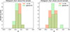 |
Fig. 7. Histogram of best-fit corrected phase shifts ϕ′ for the first pulsar sample (on the left) and the second pulsar sample (on the right). |
6. Discussion of possible misalignments
A spin-orbit alignment arises due to the accretion of matter and, thus, angular momentum from an accretion disk whose angular momentum vector is orthogonal to the orbital plane that overlaps with the accretion disk plane. The accreted angular momentum, ΔL, must be comparable to the pulsar spin angular momentum, L, to expect any significant evolution towards alignment; thus, ΔL ≈ L = I Ω, with  the moment of inertia of the pulsar (with M and R being the mass and radius of the pulsar, respectively) and Ω as the angular velocity. We assumed a homogeneous density inside the star for the computation of the moment of inertia. The evolution of the pulsar angular momentum is then given by
 (5)
(5)
with N the torque acting on the pulsar due to the accretion of matter from the companion. A simple estimate assuming a constant accretion rate of ṁ at a radius racc shows that  with the internal limit of the accretion disk designates as the accretion radius racc. Moreover, as explained in detail in Abolmasov et al. (2024), for the pulsar to be in an accretion regime, this radius must be smaller than the corotation radius, Rco, and than the gravitational capture radius, RG.
Taking a pulsar of initial mass, M0, and increasing over time as  , Eq. (5) is rewritten as
 (6)
(6)
using the fact that  . Its integration yields the general expression for the stellar angular velocity as
 (7)
(7)
with Ω0 corresponding to the initial angular velocity of the pulsar, taken to be  with P0 as its initial rotation period. The associated general expression for the angular momentum is
![Mathematical equation: $$ \begin{aligned} L(t) = I(t) \, \Omega (t) = L_0 + \frac{2}{3}\sqrt{G \, M_0^3 \, r_{\rm acc}} \left[ \left(1+\frac{\dot{m}}{M_0} \, t \right)^{3/2}-1\right] ,\end{aligned} $$](/articles/aa/full_html/2026/03/aa56461-25/aa56461-25-eq88.gif) (8)
(8)
with  the initial angular momentum. The typical alignment timescale, τalign, for which we would have a variation of the angular momentum of the order of ΔL ≈ L0 can then be estimated by
 (9)
(9)
Assuming a spherical accretion, we take for the inner radius of the accretion disk the expression (see Biryukov & Abolmasov 2021):
 (10)
(10)
where μ is the stellar magnetic moment. The latest can be estimated with the formula  , where B is the strength of the dipolar magnetic field at the equator. In this way, the previous equation can be recast as
 (11)
(11)
with ṀEdd the Eddington accretion rate. To obtain this form, we assumed that  . Indeed, in a first approximation we can write
  , with ΔM the variation of mass of the pulsar, meaning that
  . As explained in Tauris et al. (2017), the total mass accreted by the pulsar during its accretion phase represents only a small fraction of its total mass. Thus we can assume
  . The expression (11) gives an estimate of the typical time needed to reach an alignment, which is of the order of 3.8 × 10⁶ yr for typical pulsar binary parameters.
In most cases, when the accretion phase starts, the period of the pulsar will be much larger than P = 1 ms as given in the former formula, meaning that the previous result rather corresponds to an upper limit of this alignment time. By taking a more realistic value for the initial period, that is P = 5 s, we now obtain a new value for the alignment time of the order of 1 kyr. An accretion rate well below the Eddington limit could also drastically increase the alignment timescale by a factor 10–100.
To assess whether a pulsar had enough time to reach alignment during the accretion phase, we need an estimate of the total duration of that phase. For that purpose, we simulated a population of millisecond pulsars (MSPs) born in binaries with main-sequence companions, modelling their evolution using the SEVN code (Spera & Mapelli 2017; Iorio et al. 2023) to track both stellar and binary processes. The spin and magnetic evolution of pulsars was treated following the prescription of Biryukov & Abolmasov (2021). To identify detectable systems, we applied a detection pipeline closely following Sautron et al. (2024), accounting for selection effects in both radio (at 1.4 GHz) and γ-ray bands, based on Fermi/LAT sensitivity. Full details of the simulation and detection methodology are presented in Sautron et al. (2026). One of the outcomes of the simulation, which involved 580 000 binaries and led to 519 detections (either in radio or γ-ray, or both) that matched the observations in the P−Ṗ diagram, with only 240 pulsars remaining in binaries, is plotted in Figure 8. This figure shows the number of pulsars left at the end of the simulation depending on the angle α between the rotation axis and the orbital angular momentum of the binary, indicated on the horizontal axis, and on the duration of the accretion phase, indicated on the vertical axis. For the large majority of pulsars, the duration of the accretion phase is about 108 − 9 yr, thus much larger than the orders of magnitude we found for the alignment time in the previous calculation. For this reason, we expect most of the pulsars to reach alignment during the accretion phase. Figure 8 also confirms that point, since almost all pulsars ended with an angle α situated between 0° and 10°, after an accretion regime of duration 108 − 9 yr. However, 20% of the simulated pulsars finished their accretion phase with a residual angle α superior to 10°. If we exclude the pulsars for which the misalignment we found most probably comes from some limitations of our γ-ray light curve model, it seems indeed possible that several MSPs are misaligned in our sample.
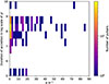 |
Fig. 8. Spin-orbit inclination angle, α, of a simulated population of MSPs that are still in a binary after the end of the accretion phase. The majority of MSPs show close to alignment geometries after tens of millions of years. |
7. Conclusion
In this work, we study recycled pulsars that are spun up by accretion of matter from their companion in a binary system, known as MSPs. This spin-up is accompanied by a torque that tends to align the stellar spin with the orbital angular momentum vector on a rather short timescale. As they are old pulsars with ages of around a billion year, they have had enough time to align their spin with the orbit. This hypothesis has been checked in our work by computing the pulsar viewing angle from γ-ray light curve fitting. By using two samples, one with accurate measurements of the orbital inclination angle, i, and another with some constraints on the possible intervals, we found that about four-fifths of the MSPs indeed show spin-orbit alignment within several degrees. However, a small sub-sample could not be accommodated with this hypothesis; thus, we conclude that either our γ-ray light curve modelling is inaccurate or they indeed are largely misaligned. Such a possible misalignment was found in our MSP population synthesis simulation, where a small fraction of pulsars still have a discrepancy greater than 10° between the rotation axis and normal to the orbital plane. The origin of this misalignment must be accounted for via the accretion history and the initial condition prior the accretion regime. However, such a detailed analysis of the binary evolution and outcome will be the focus of a forthcoming investigation based on MSP population synthesis.
Acknowledgments
This work has been supported by the French Research Agency grant ANR-20-CE31-0010. We are grateful to our referee for his/her helpful comments.
References
- Abolmasov, P., Biryukov, A., & Popov, S. B. 2024, Galaxies, 12, 7 [NASA ADS] [CrossRef] [Google Scholar]
- Andrae, R., Schulze-Hartung, T., & Melchior, P. 2010, arXiv e-prints [arXiv:1012.3754] [Google Scholar]
- Arzoumanian, Z., Baker, P. T., Brazier, A., et al. 2018, ApJ, 859, 47 [NASA ADS] [CrossRef] [Google Scholar]
- Ashton, G., Hübner, M., Lasky, P. D., et al. 2019, ApJS, 241, 27 [NASA ADS] [CrossRef] [Google Scholar]
- Bai, X.-N., & Spitkovsky, A. 2010, ApJ, 715, 1282 [Google Scholar]
- Benli, O., Pétri, J., & Mitra, D. 2021, A&A, 647, A101 [NASA ADS] [CrossRef] [EDP Sciences] [Google Scholar]
- Biryukov, A., & Abolmasov, P. 2021, MNRAS, 505, 1775 [NASA ADS] [CrossRef] [Google Scholar]
- Blanchard, C., Guillemot, L., Voisin, G., Cognard, I., & Theureau, G. 2025, A&A, 698, A239 [NASA ADS] [CrossRef] [EDP Sciences] [Google Scholar]
- Breton, R. P., van Kerkwijk, M. H., Roberts, M. S. E., et al. 2013, ApJ, 769, 108 [Google Scholar]
- Cao, G., & Yang, X. 2019, ApJ, 874, 166 [Google Scholar]
- Cao, G., & Yang, X. 2022, ApJ, 925, 130 [Google Scholar]
- Cerutti, B., Philippov, A. A., & Spitkovsky, A. 2016, MNRAS, 457, 2401 [Google Scholar]
- Cerutti, B., Figueiredo, E., & Dubus, G. 2025, A&A, 695, A93 [NASA ADS] [CrossRef] [EDP Sciences] [Google Scholar]
- Choudhury, D., Salmi, T., Vinciguerra, S., et al. 2024, ApJ, 971, L20 [NASA ADS] [CrossRef] [Google Scholar]
- Clark, C. J., Kerr, M., Barr, E. D., et al. 2023, Nat. Astron., 7, 451 [NASA ADS] [CrossRef] [Google Scholar]
- Contopoulos, I., & Kalapotharakos, C. 2010, MNRAS, 404, 767 [Google Scholar]
- Desvignes, G., Caballero, R. N., Lentati, L., et al. 2016, MNRAS, 458, 3341 [Google Scholar]
- Dittmann, A. J., Miller, M. C., Lamb, F. K., et al. 2024, ApJ, 974, 295 [NASA ADS] [CrossRef] [Google Scholar]
- Draghis, P., Romani, R. W., Filippenko, A. V., et al. 2019, ApJ, 883, 108 [NASA ADS] [CrossRef] [Google Scholar]
- Fonseca, E., Pennucci, T. T., Ellis, J. A., et al. 2016, ApJ, 832, 167 [Google Scholar]
- Fonseca, E., Cromartie, H. T., Pennucci, T. T., et al. 2021, ApJ, 915, L12 [NASA ADS] [CrossRef] [Google Scholar]
- Gautam, T., Freire, P. C. C., Wu, J., et al. 2024, A&A, 682, A103 [NASA ADS] [CrossRef] [EDP Sciences] [Google Scholar]
- Gendreau, K. C., Arzoumanian, Z., & Okajima, T. 2012, Space Telescopes and Instrumentation 2012: Ultraviolet to Gamma Ray, 8443, 844313 [CrossRef] [Google Scholar]
- Guillemot, L., & Tauris, T. M. 2014, MNRAS, 439, 2033 [NASA ADS] [CrossRef] [Google Scholar]
- Hui, C. Y., & Li, K. L. 2019, Galaxies, 7, 93 [NASA ADS] [CrossRef] [Google Scholar]
- Iorio, G., Mapelli, M., Costa, G., et al. 2023, MNRAS, 524, 426 [NASA ADS] [CrossRef] [Google Scholar]
- Jacovitti, G., & Scarano, G. 1993, IEEE Trans. Signal Process., 41, 417 [Google Scholar]
- Kalapotharakos, C., Harding, A. K., & Kazanas, D. 2014, ApJ, 793, 97 [Google Scholar]
- Kalapotharakos, C., Brambilla, G., Timokhin, A., Harding, A. K., & Kazanas, D. 2018, ApJ, 857, 44 [NASA ADS] [CrossRef] [Google Scholar]
- Kalapotharakos, C., Wadiasingh, Z., Harding, A. K., & Kazanas, D. 2023, ApJ, 954, 204 [NASA ADS] [CrossRef] [Google Scholar]
- Kaplan, D. L., Stovall, K., van Kerkwijk, M. H., Fremling, C., & Istrate, A. G. 2018, ApJ, 864, 15 [Google Scholar]
- Kirk, J. G., Skjæraasen, O., & Gallant, Y. A. 2002, A&A, 388, L29 [NASA ADS] [CrossRef] [EDP Sciences] [Google Scholar]
- Kramer, M., & Johnston, S. 2025, MNRAS, accepted [arXiv:2510.05778] [Google Scholar]
- Kramer, M., Stairs, I., Manchester, R., et al. 2021, Phys. Rev. X, 11, 041050 [NASA ADS] [Google Scholar]
- Laycock, S. G. T., Cappallo, R. C., Pradhan, P., Christodoulou, D. M., & Paul, B. 2025, ApJ, 978, 80 [Google Scholar]
- Lewis, J. P. 1995, Vision Interface (Industrial Light& Magic), 120 [Google Scholar]
- Li, M., Halpern, J. P., & Thorstensen, J. R. 2014, ApJ, 795, 115 [NASA ADS] [CrossRef] [Google Scholar]
- Löhmer, O., Lewandowski, W., Wolszczan, A., & Wielebinski, R. 2005, ApJ, 621, 388 [Google Scholar]
- Lorimer, D. R. 2008, Liv. Rev. Relat., 11, 8 [Google Scholar]
- Mata Sánchez, D., Kennedy, M. R., Clark, C. J., et al. 2023, MNRAS, 520, 2217 [CrossRef] [Google Scholar]
- Miller, M. C., Lamb, F. K., Dittmann, A. J., et al. 2019, ApJ, 887, L24 [Google Scholar]
- Miller, M. C., Lamb, F. K., Dittmann, A. J., et al. 2021, ApJ, 918, L28 [NASA ADS] [CrossRef] [Google Scholar]
- Ng, C., Guillemot, L., Freire, P. C. C., et al. 2020, MNRAS, 493, 1261 [Google Scholar]
- Pétri, J. 2011, MNRAS, 412, 1870 [Google Scholar]
- Pétri, J. 2012, MNRAS, 424, 605 [Google Scholar]
- Pétri, J. 2024, A&A, 687, A169 [NASA ADS] [CrossRef] [EDP Sciences] [Google Scholar]
- Pétri, J., & Mitra, D. 2021, A&A, 654, A106 [NASA ADS] [CrossRef] [EDP Sciences] [Google Scholar]
- Philippov, A. A., & Spitkovsky, A. 2018, ApJ, 855, 94 [NASA ADS] [CrossRef] [Google Scholar]
- Polzin, E. J., Breton, R. P., Bhattacharyya, B., et al. 2020, MNRAS, 494, 2948 [Google Scholar]
- Press, W. H., Teukolsky, S. A., Vetterling, W. T., & Flannery, B. P. 2007, Numerical Recipes 3rd Edition: The Art of Scientific Computing [Google Scholar]
- Reardon, D. J., Hobbs, G., Coles, W., et al. 2016, MNRAS, 455, 1751 [NASA ADS] [CrossRef] [Google Scholar]
- Riley, T. E., Watts, A. L., Bogdanov, S., et al. 2019, ApJ, 887, L21 [Google Scholar]
- Salmi, T., Choudhury, D., Kini, Y., et al. 2024, ApJ, 974, 294 [NASA ADS] [CrossRef] [Google Scholar]
- Sautron, M., Pétri, J., Mitra, D., & Dirson, L. 2024, A&A, 691, A349 [NASA ADS] [CrossRef] [EDP Sciences] [Google Scholar]
- Sautron, M., Pétri, J., Mitra, D., Dupuy-Junet, A., & Pietrin, M.-E. 2026, A&A, 707, A257 [NASA ADS] [CrossRef] [EDP Sciences] [Google Scholar]
- Serylak, M., Venkatraman Krishnan, V., Freire, P. C. C., et al. 2022, A&A, 665, A53 [NASA ADS] [CrossRef] [EDP Sciences] [Google Scholar]
- Shamohammadi, M., Bailes, M., Freire, P. C. C., et al. 2023, MNRAS, 520, 1789 [NASA ADS] [CrossRef] [Google Scholar]
- Smith, D. A., Abdollahi, S., Ajello, M., et al. 2023, ApJ, 958, 191 [NASA ADS] [CrossRef] [Google Scholar]
- Spera, M., & Mapelli, M. 2017, MNRAS, 470, 4739 [Google Scholar]
- Tan, C. M., Fonseca, E., Crowter, K., et al. 2024, ApJ, 966, 26 [Google Scholar]
- Tauris, T. M., Kramer, M., Freire, P. C. C., et al. 2017, ApJ, 846, 170 [Google Scholar]
- van der Wateren, E., Bassa, C. G., Clark, C. J., et al. 2022, A&A, 661, A57 [NASA ADS] [CrossRef] [EDP Sciences] [Google Scholar]
- Vigeland, S. J., & Vallisneri, M. 2014, MNRAS, 440, 1446 [NASA ADS] [CrossRef] [Google Scholar]
- Yang, H.-r., & Li, X.-d. 2023, ApJ, 945, 2 [Google Scholar]
Appendix A: Fitting process
In this section, we explain how to analyse an observed γ-ray light curve obtained from the Fermi/LAT telescope. Such curve is a discrete signal u = (u[k],k = 0, …, N − 1), each measurement u[k] being associated with a corresponding phase φ[k]=k/N. The Fermi data set provides N measurement points, with the number of points N varying depending on the luminosity of each pulsar. For the brightest pulsars of our sample, N can reach 100 but can also go below 30 for faint pulsars with poor photon statistics.
A.1. Fitting method
In previous sections, we explain that the shape of such a signal depends on the geometry of the pulsar, which is described by a couple of angles θ = (χ, ζ); to be admissible, the parameter, θ, must belong to
![Mathematical equation: $$ \begin{aligned} \Theta =\{(\chi ,\zeta ) \in [0,\frac{\pi }{2}]^2 : |\zeta - \frac{\pi }{2}| \le \chi \text{ and} |\zeta - \chi | \le \rho \} ,\end{aligned} $$](/articles/aa/full_html/2026/03/aa56461-25/aa56461-25-eq98.gif) (A.1)
(A.1)
with ρ the half-opening angle of the radio beam cone.
For each parameter θ = (χ, ζ), a modelled continuous signal Vθ(φ) is available for analysis. We use vθ to denote its discretisation vθ[k]=Vθ(φk).
We remark that our numerical process gives the function φ → Vθ(φ) at some phases that are not the φk. An interpolation via Fourier series allows us to evaluate it precisely at the φk.
The collection {vθ : θ ∈ Θ} constitutes the atlas encompassing all possible discrete signal shapes. An illustration of this atlas is given in Pétri (2024). The observed signal u must be a noisy variant of one of the signals within this atlas, subject to three transformations: phase-shift, spatial scaling (intensity normalisation), and spatial translation (background level).
To be more precise, for a discrete signal, v, we use vt to denote its phase-shifted version: vt[k]=v[k − t] (the minus sign being considered modulo N because of the periodicity of the signal). Our purpose is to find parameters,
 (A.2)
(A.2)
so that
 (A.3)
(A.3)
We solve this problem in two steps:
First step: For a given θ ∈ Θ, the normalized-cross-correlation methods (see Appendix B) allows us to find efficiently the triplet  minimizing ||u − (avtθ + b)||2 . The fitted signal is denoted by:
 (A.4)
(A.4)
We express f(k, θ) = f(θ)[k] for the fitted signal at phase φ[k].
Second step: We suppose that each measure u[k] is obtained by adding to f(k, θ) a Gaussian noise with a known standard deviation σk (known from the Fermi data set).
So u[k] is viewed as a sample of a random variable with density:
 (A.5)
(A.5)
Assuming that the noises are independent from one measurement to the next, the entire observed signal u is regarded as a sample from a random vector with density,
 (A.6)
(A.6)
where y = (y0, …, yN − 1) represents the generic element of  . Taking the logarithm of the expression above yields
 (A.7)
(A.7)
We note that the left term of the difference above does not depend on the parameter θ and will be ignored during the optimization process below.
Within the Bayesian framework, it is postulated that the parameter, θ, follows a prior distribution denoted as π(θ) (two options for such a distribution are described subsequently). The Bayes’ theorem provides a formulation for the posterior distribution of θ given y
 (A.8)
(A.8)
The denominator term p(y) = ∫Θp(y|θ)π(θ) dθ is referred to as the evidence. Its calculation is irrelevant because it does not depend on θ.
To determine the parameter  that renders the observed signal u the most realistic among all possible parameters θ ∈ Θ, we need to maximize the posterior probability evaluated at y = u so we have to find
  . Considering the log-expression (A.7), the optimization problem can be simplified to
![Mathematical equation: $$ \begin{aligned} \hat{\theta } = \arg \min _{\theta \in \Theta }\left[ \frac{1}{2} \sum _{k = 0}^{N-1}\frac{(u[k] - f(k, \theta ))^2}{\sigma _k^2} - \log \pi (\theta ) \right] \ . \end{aligned} $$](/articles/aa/full_html/2026/03/aa56461-25/aa56461-25-eq110.gif) (A.9)
(A.9)
To enhance the importance of measurements at the signal’s peak, we introduced a weighting factor to the previously stated expression,
![Mathematical equation: $$ \begin{aligned} \hat{\theta } = \arg \min _{\theta \in \Theta }\left[ \frac{1}{2} \sum _{k = 0}^{N-1}\frac{(u[k]+1)^2 (u[k] - f(k, \theta ))^2}{\sigma _k^2} - \log \pi (\theta ) \right] \ . \end{aligned} $$](/articles/aa/full_html/2026/03/aa56461-25/aa56461-25-eq111.gif) (A.10)
(A.10)
We observe that the preceding adjustment is equivalent to substituting σi with ![Mathematical equation: $ \frac{\sigma_i}{u[i]+1} $](/articles/aa/full_html/2026/03/aa56461-25/aa56461-25-eq112.gif) ; thus, supposing that the measurements on the peaks are less susceptible to noise interference.
; thus, supposing that the measurements on the peaks are less susceptible to noise interference.
Finally, to determine the minimum, a finite grid Θ′⊂Θ is selected and evaluate all quantities (A.10) for θ ∈ Θ′. This task is facilitated by the fact that Θ is a simple sub-set of ℝ2 and by the computational efficiency of the function, f, via the normalized cross-correlation method.
However, for our simple 2D optimization problem, the employed grid method facilitates the rapid identification of the minimum with high precision. We utilized a grid with variations at one-degree increments in χ and ζ, granularity could be extended if necessary.
A.2. Application to the Shapiro delay
We applied the previous process with two different priors:
First prior:π the isotropic distribution over Θ (in other word, the uniform distribution of the restricted part of the sphere).
Second prior: Considering the orbital inclination, i,
 (A.11)
with Cχ a normalization factor so that the density has integral is 1. We note that this constant depends on χ because the domain is not rectangular. However, for the parameters that we estimated, the Gaussian is peaked enough so that this dependence can be neglected. Thus, this multiplicative constant vanishes during the optimization process.
A.3. Example of two fitting results
The fitting procedure leads to corner plots as an output, of which an example is shown in Fig. A.1 for two pulsars. On the left panel, for pulsar J0740+6620 and on the right panel for J1514−4946. The error bars on the two characteristic angles are deduced from the quartiles at 99.85% and 0.15%, corresponding to a 3 σ confidence interval. For J0740+6620 which is an example of a good fitting, the p-value passes the KS test. However, as a less accurate fitting example, we also show J1514−4946, on the right panel of Fig. A.1.
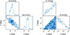 |
Fig. A.1. Corner plots for the fitting in the general case, without Shapiro constraint, for pulsar J0740+6620 on the left panel, and for pulsar J1514−4946 on the right panel. |
A.4. Pulsars with a retained symmetrical solution
To demonstrate the small impact of taking an almost symmetrical solution for the γ-ray fitting, we show here the light curves using the θbest fit that minimize  on the whole parameter space for PSR J0955−6150, J1012−4235, J1713+0747 from the first sample (see Fig. A.2) and for PSR J0101−6422, J1514−4946, J2051−0827 and J2256−1024 from the second sample (see Fig. A.3). The feature of these light curves are indeed very similar to the one obtained by swapping the angles χ and ζ.
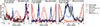 |
Fig. A.2. Original solution for pulsars from the first sample for which the symmetrical solution has been kept. |
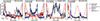 |
Fig. A.3. Original solution for pulsars from the second sample for which the symmetrical solution has been kept. |
Appendix B: The cross-correlation method
In this section, we explain the principle of the normalized cross-correlation as delineated in Lewis (1995) and Jacovitti & Scarano (1993). We substantiate this method through a concise mathematical proof, tailored specifically to our context.
B.1. Principle
We consider u and v as two discrete periodic signals of length N. We define vt as the time-shifted signal ![Mathematical equation: $ v_{t}[k] = v[k-t] $](/articles/aa/full_html/2026/03/aa56461-25/aa56461-25-eq115.gif) , where the minus operation is performed modulo N due to the periodicity. Our objective is to apply three transformations to v, namely: time-shift, spatial translation, and spatial scaling, such that it aligns as closely as possible with the signal u. This objective is quantitatively accomplished by minimizing the following expression,
, where the minus operation is performed modulo N due to the periodicity. Our objective is to apply three transformations to v, namely: time-shift, spatial translation, and spatial scaling, such that it aligns as closely as possible with the signal u. This objective is quantitatively accomplished by minimizing the following expression,
![Mathematical equation: $$ \begin{aligned} \Vert u - (a \, v_t + b)\Vert ^2= \sum _k \big (u[k] - a \, v[k-t] - b\big )^2 ,\end{aligned} $$](/articles/aa/full_html/2026/03/aa56461-25/aa56461-25-eq116.gif) (B.1)
(B.1)
over all possible parameters  .
.
Proposition: Let us define the centred versions of our signals as  and
and  . The minimizers of ∥u − (a vt + b)∥2 are given by
  where
where  and
and  are the location and the value of the maximum of the function,
![Mathematical equation: $$ \begin{aligned} t\rightarrow \frac{1}{K} \sum _k \dot{u}[k] \dot{v}[k-t] \qquad \text{ with} K=\sum _k (\dot{v}[k])^2 ,\end{aligned} $$](/articles/aa/full_html/2026/03/aa56461-25/aa56461-25-eq123.gif) (B.2)
(B.2)
and where  .
.
Observation: The function B.2 is called the cross-correlation, and is calculated efficiently utilizing the fast Fourier transform (FFT) algorithm. The comprehensive algorithm is detailed in the concluding sub-section.
B.2. Proof
To establish the proposition, we reduce to the case where the signals are centred, with the help of the following lemma.
Lemma: The minimizers  of
of  are linked to the minimizers
  of ∥u − a vt − b∥2 by
 (B.3)
(B.3)
with  .
.
Proof of the lemma: Injecting  in the expression they need to minimize, we get
 (B.4)
(B.4)
which is actually the minimal possible value from the very definition of the triplet  . ▫
. ▫
Building upon this lemma, it becomes sufficient to demonstrate the proposition within the context where u and v have already been centred. For the remainder of the proof, we will operate under this assumption, thus rendering the dot notations unnecessary.
Proof of the proposition: Initially, we address the minimization problem for a specified value of t. Thus, we seek
This is a classical least squares problem that is resolved utilizing the normal equation. The details are as follows: we let Vt represent the matrix wherein the first column consists of coefficients equal to 1, and the second column is the vector, vt. We let U denote the matrix comprising a single column, which is the vector u. According to the normal equation, the solution to B.2 is provided by
Given that both u and v have been centred, the calculation process is straightforward
![Mathematical equation: $$ \begin{pmatrix} \hat{b}_t \\ \hat{a}_t \end{pmatrix}= \begin{pmatrix} 0 \\ \frac{1}{K} \sum _k u[k] \, v[k-t] \end{pmatrix} \ . $$](/articles/aa/full_html/2026/03/aa56461-25/aa56461-25-eq135.gif)
Now, to find the t-minimizer, we have to minimize  . We develop
![Mathematical equation: $$ \begin{aligned} \hat{t}&= \underset{t}{\text{ argmin}}\sum _k\Big ( u[k] - \hat{a}_t \, v_t[k] \Big )^2, \\&= \underset{t}{\text{ argmin}}\Big [ \sum _k (u[k])^2 + (\hat{a}_t)^2 (v[k-t])^2 - 2 \, u[k] \, \hat{a}_t \, v[k-t] \Big ],\\&= \underset{t}{\text{ argmin}} \Big [(\hat{a}_t)^2 \sum _k (v[k-t])^2 - 2 \, \hat{a}_t \sum _k u[k] \, v[k-t] \Big ],\\&= \underset{t}{\text{ argmin}} \Big [(\hat{a}_t)^2 K - 2 \hat{a}_t \, K \, \hat{a}_t\Big ],\\&= \underset{t}{\text{ argmax}}\ (\hat{a}_t)^2 = \underset{t}{\text{ argmax}}\ \hat{a}_t, \end{aligned} $$](/articles/aa/full_html/2026/03/aa56461-25/aa56461-25-eq137.gif)
which concludes the proof of the proposition. ▫
B.3. Algorithm
Analogously to mathematical reasoning, the algorithm reduces to the case where vectors u and v are centred. For concreteness, we give Python code to perform this cross-correlation.
from numpy.fft import fft,ifft
from numpy import mean,sum,roll,flip,argmax,real
Listing 1. Python import
def find_best_shift_scaling_for_centred(u, v):
#v_inverse[i]=v[-i] (with periodicity)
v_inverse = roll(flip(v), 1)
K = sum(v ** 2)
cross_correlation = real(ifft(fft(u) * fft(
v_inverse))) / K
t = argmax(cross_correlation)
a = cross_correlation[t]
return t, a
Listing 2. Preliminary function: which suppose that inputs u and v are centred
def find_best_shift_scaling_translation(u, v):
mean_u = mean(u)
mean_v = mean(v)
t, a = find_best_shift_scaling_for_centred(u -
mean_u, v - mean_v)
b = mean_u - a * mean_v
return t, a, b
Listing 3. Final function using the previous one.
Figure B.1 shows an example of fitting to a periodic and double peaked signal. To draw this plot, we compute u by taking φ, a vector of 200 phases from 0 to 2π. Then, we derive x = cos(φ),y = sin(φ). Finally, we set u = g(x − 1, y)+3g(x + 1, y) where g(x, y) = exp(−(x2 + y2)/σ2) is a Gaussian curve with a small standard deviation σ2 = 0.1.
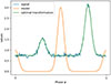 |
Fig. B.1. Graphical evaluation of the proposed algorithm. The orange curve represents a periodic signal modeling a reference signal from our atlas. The blue curve denotes a noisy signal corresponding to an observed measurement. The green curve illustrates the optimal transformation of the orange signal, obtained through temporal shifts, spatial shift and amplitude scaling, which best matches the blue signal. |
All Tables
All Figures
|
Fig. 1. Light curve fitting from the first sample of MSPs, with the black curve and the dark red curves corresponding to the γ-ray and radio data, respectively. The light blue and the orange curves correspond to the γ-ray light curves and radio profiles, respectively. Finally, the light blue dotted and orange dotted curves obtained from the same fitting, but imposing a perfect alignment, signifying ζ = i. |
| In the text | |
|
Fig. 2. Histogram of the best-fit parameters cos χ (left), cos ζ (middle), and ϕ (right) for the first sample of MSPs, in green in the general case and in orange for the fitting imposing i = ζ. |
| In the text | |
|
Fig. 3. Left: χ−ζ plane showing the best-fit couple of angles χ and ζ for the first sample of MSPs. Right: ζ − i plane showing the best-fit angle, ζ, for the inclination, i, imposed by Shapiro delay measurements, with the blue dotted line corresponding to the perfect alignment condition i = ζ. Individual pulsars are depicted by different colours. |
| In the text | |
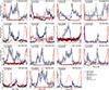 |
Fig. 4. Same as in Fig. 1, but for the second sample of MSPs. |
| In the text | |
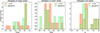 |
Fig. 5. Same as Fig. 2, but for the second sample of MSPs. |
| In the text | |
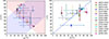 |
Fig. 6. Same as Fig. 6, but for the second sample of MSPs. |
| In the text | |
|
Fig. 7. Histogram of best-fit corrected phase shifts ϕ′ for the first pulsar sample (on the left) and the second pulsar sample (on the right). |
| In the text | |
|
Fig. 8. Spin-orbit inclination angle, α, of a simulated population of MSPs that are still in a binary after the end of the accretion phase. The majority of MSPs show close to alignment geometries after tens of millions of years. |
| In the text | |
|
Fig. A.1. Corner plots for the fitting in the general case, without Shapiro constraint, for pulsar J0740+6620 on the left panel, and for pulsar J1514−4946 on the right panel. |
| In the text | |
|
Fig. A.2. Original solution for pulsars from the first sample for which the symmetrical solution has been kept. |
| In the text | |
|
Fig. A.3. Original solution for pulsars from the second sample for which the symmetrical solution has been kept. |
| In the text | |
|
Fig. B.1. Graphical evaluation of the proposed algorithm. The orange curve represents a periodic signal modeling a reference signal from our atlas. The blue curve denotes a noisy signal corresponding to an observed measurement. The green curve illustrates the optimal transformation of the orange signal, obtained through temporal shifts, spatial shift and amplitude scaling, which best matches the blue signal. |
| In the text | |
Current usage metrics show cumulative count of Article Views (full-text article views including HTML views, PDF and ePub downloads, according to the available data) and Abstracts Views on Vision4Press platform.
Data correspond to usage on the plateform after 2015. The current usage metrics is available 48-96 hours after online publication and is updated daily on week days.
Initial download of the metrics may take a while.