| Issue |
A&A
Volume 707, March 2026
|
|
|---|---|---|
| Article Number | A310 | |
| Number of page(s) | 13 | |
| Section | Galactic structure, stellar clusters and populations | |
| DOI | https://doi.org/10.1051/0004-6361/202556723 | |
| Published online | 23 March 2026 | |
Dynamical mirages: How bar-induced resonant trapping can mimic substructure clustering in dynamical parameter spaces
1
Dipartimento di Fisica e Astronomia, Università degli Studi di Bologna,
Via Piero Gobetti 93/2,
Bologna
40129,
Italy
2
Osservatorio di Astrofisica e Scienza dello Spazio di Bologna, INAF,
Via Piero Gobetti 93/3,
Bologna
40129,
Italy
3
Instituto de Astrofísica, Pontificia Universidad Católica de Chile,
Av. Vicuña Mackenna 4860,
782-0436
Macul, Santiago,
Chile
4
Instituto Milenio de Astrofísica MAS,
Av. Vicuña Mackenna 4860,
782-0436
Macul, Santiago,
Chile
★ Corresponding author: This email address is being protected from spambots. You need JavaScript enabled to view it.
Received:
2
August
2025
Accepted:
6
November
2025
Abstract
Context. The complex task of unraveling the assembly history of the Milky Way evolves constantly, and new substructures are identified continuously. To properly validate and characterise the family of galactic progenitors, it is important to take all the effects into account that can shape the distribution of tracers in the Galaxy. First among the often overlooked actors of galactic dynamics is the rotating bar of the Milky Way, which can affect orbital tracers in multiple ways.
Aims. We wish to fully characterise the effect of the rotating bar of the Milky Way on the distribution of galactic tracers, provide diagnostics that can help to identify its effect and explore the implications for the search and identification of substructures.
Methods. We used the in-house code Orbital Integration Tool (ORBIT), built to include the full effect of the bar and exploit its multidimensional output to perform a complete dynamical characterisation of a large sample of carefully selected Milky Way stars with very precise astrometry.
Results. We identified conspicuous overdensities in several orbital parameter spaces and verified that they are caused by the bar-induced resonances. We also show that contamination by trapped tracers provides local density enhancements that mimic the clumping usually attributed to genuine substructures.
Conclusions. We provide a new and fast way of identifying resonant loci and consequently, of estimating the contribution of stars trapped into orbital resonances to phase-space overdensities that were previously identified as candidate relics of past merging events. Among those analysed here, we found that the detections of Cluster 3 and Shakti seem to have gained a non-negligible boost from resonance-trapped stars. Nyx is the most extreme case, with ~70% of the assigned member stars lying on resonant orbits. This strongly suggests that it is not a genuine merger relic but is instead an overdensity caused by bar-induced resonances.
Key words: methods: numerical / celestial mechanics / Galaxy: evolution / Galaxy: kinematics and dynamics / Galaxy: structure
© The Authors 2026
 Open Access article, published by EDP Sciences, under the terms of the Creative Commons Attribution License (https://creativecommons.org/licenses/by/4.0), which permits unrestricted use, distribution, and reproduction in any medium, provided the original work is properly cited.
This article is published in open access under the Subscribe to Open model. This email address is being protected from spambots. You need JavaScript enabled to view it. to support open access publication.
1 Introduction
The study of the evolution and structure of the Milky Way (MW) is continuously ongoing. The premier technique used to identify structures, moving groups and candidate relics of ancient merger events is to search for overdensities and clumps in integrals of motion (IoMs) spaces (chiefly the angular momentum vs energy space, Lz–Etot; Helmi & de Zeeuw 2000) or in the action spaces (i.e. Myeong et al. 2018). The recovery of these orbital parameters is model dependent because it is based on the underlying potential used to reconstruct the orbital history of the tracers. The technique of orbit integration sits at the crossroad of observations and theory as it uses observed starting positions and velocities of tracers and the theoretical model of a density distribution to compute the forces that dictate the motions of the tracers and reconstruct their orbits. Modeling of structure in simulations closely follows observational evidence, with complex multi-component potential distributions that aim to reproduce the density of both the observed luminous matter and the inferred dark matter (DM). The same cannot be said for the models used for orbital integration. Most studies are still conducted using underlying static, axisymmetric potential models. These remove the ability to identify the effects deriving from a time-varying potential, such as the secular evolution of the MW and the effect of its rotating bar. The latter in particular has a multifaceted influence on the dynamics of galactic tracers, from the non-conservation of some IoMs to the shepherding and trapping of tracers in resonances. Theoretical predictions of the action of the bar are plentiful in the literature, starting from the effect it might have on the disc (Kalnajs 1991; McMillan 2013; Chiba et al. 2021; Chiba & Schönrich 2021), on the stellar halo (Moreno et al. 2015, 2021) and on the DM halo (Debattista & Sellwood 1998, 2000). One of the first examples of a peculiar moving group linked to the effect of the bar was the Hercules group (Eggen 1958; Dehnen 2000; Pérez-Villegas et al. 2017; D’Onghia & Aguerri 2020). Initially associated with the outer Lindblad resonance under models of a fast-rotating, small bar (i.e. Dehnen 2000, with Ωp = 55 km s−1 kpc−1, abar = 3 kpc), later studies have shown it is trapped around the fourth Lagrangian point, a stable region along the bar minor axis, around the corotation resonance (i.e. D’Onghia & Aguerri 2020, with Ωp = 40 km s−1 kpc−1, abar = 4.5 kpc). The advent of the Gaia catalogues (Gaia Collaboration 2016), with their unprecedented volume of data, opened up the possibility of a detailed and statistically meaningful analysis of stellar kinematics. This led to a more systematic study of the effect of the bar-induced resonances on tracer populations (Khoperskov et al. 2020; Khoperskov & Gerhard 2022; Dillamore et al. 2023, Dillamore et al. 2024b,a). At the same time, more sophisticated clustering techniques and algorithms led to the identification of new substructures (i.e. for some of the latest developments; Lövdal et al. 2022; Ruiz-Lara et al. 2022; Dodd et al. 2023; Liu et al. 2024). The debate on the validation of substructures (both new and previously identified) with dynamical information is in full swing, with very recent works (Woudenberg & Helmi 2025; Dillamore & Sanders 2025) warning of the dangers of employing clustering algorithms on the Lz–Etot plane without accounting fully for the bar. One key question that remains unanswered is whether the bar-induced resonances can affect the distribution of tracers in dynamical phase spaces profoundly enough to contaminate or even mimic the presence of a real substructure.
With the aim of studying the full effect of the rotating bar on the dynamics of MW tracers, we explored the dynamical parameter space of a large sample of MW stars with exquisite astrometry (Bellazzini et al. 2023a, fully presented in Sect. 2). We conducted our study with the code ORBIT (De Leo et al. 2026), which was developed to fully account for the effect of the rotating bar and is described together with its underlying potential model in Section 3. Section 4 contains our findings for the main sample, and in Sect. 5 we extend our study to a selection of known substructures of the MW. We discuss our results in Section 6 and summarise them in our conclusions (Sect. 7).
2 Data
The main sample we analysed was presented in Bellazzini et al. (2023a) and is available as a public catalogue (Bellazzini et al. 2023b). Briefly, the sample is composed of 694233 red giant branch stars from the Gaia Synthetic Photometry Catalogue (GSPC, Gaia Collaboration 2023a) selected excluding probable binary, variable, and highly extincted sources and non-genuine giants. For the purposes of our work, the main characteristic of the catalogue is the exquisite astrometry deriving from the quality cuts on parallax_over_error > 10, RUWE < 1.3 (Lindegren et al. 2021b) and ≃90% of the stars with radial velocity measurements with a precision better than 3.0 km/s. These selections ensure a high standard of precision in all phase-space coordinates (α, δ, D, μRA, μDec, and RV), and the quality of the parallaxes in turn ensures a precise recovery of distance and proper motion measurements. The quality of the selected sample and the statistical nature of our analysis ensure that the observational uncertainties do not affect our results but we nevertheless include a test with maximum errors in Sect. 4.
3 Method
This work was conducted mainly using the custom-made orbit integration code ORBIT, presented and detailed in De Leo et al. (2026). Briefly, ORBIT is a code for orbit integrations written in the computing language C and using a “kick-drift-kick” integration scheme (a modified type of Verlet integration scheme, Verlet 1967; Binney & Tremaine 2008) that is timereversible and suppresses numerical errors (Roberts & Quispel 1992; Hairer et al. 2003). For our purposes, the main and most important difference between ORBIT and other publicly available codes like GALPY (Bovy 2015) or AGAMA (Action-based Galaxy Modelling Architecture Vasiliev 2019) lies in the way it accounts for the time variability of the potential underlying the integration. In particular, ORBIT computes one value of Rperi and Rapo (and therefore ecc) for each individual orbit for each tracer and the final output values are the mean of these distributions, with the standard deviations as associated errors. Thus, ORBIT accounts for the fact that the time variability of the barred potential implies that each individual radial oscillation (i.e. a single passage from pericentre to apocentre) of each tracer is slightly different from the previous ones, which makes it difficult to gauge the precision of the orbital parameters given in output as a single value. While theoretically there is no obstacle to computing the orbital parameters in this way with GALPY and AGAMA (as shown in the example with AGAMA in Fig. 3 and discussed in Sect. 4), it would require the users to step back and analyse the “raw” orbits produced by the codes on their own. Thus, the strength of ORBIT mostly lies in readily providing the outputs needed to conduct the present study.
To provide ORBIT with starting positions and velocities for the tracers, we transformed the observed positions, distances, proper motions and radial velocities to the Galactocentric reference frame. The transformation was made assuming the velocity vector of the Sun to be (U⊙, V⊙, W⊙) = (11.1, 12.24, 7.25) km s−1 (Schönrich et al. 2010), the velocity of the local standard of rest VLSR = 232.8 km s−1 (McMillan 2017), the distance of the Sun from the Galactic centre R⊙ = 8.20 kpc (GRAVITY Collaboration 2019), and the height of the Sun above the Galactic plane z⊙ = 14 pc (Binney et al. 1997). Finally, the orbital history of the tracer stars we examined was computed with ORBIT backwards in time for a total of 5 Gyr with a timestep of 103 yr.
3.1 Galactic potential model
The MW potential underlying the ORBIT integrations is a time-varying model including several components, for a detailed description see De Leo et al. (2026). Briefly, the MW is represented by a Navarro-Frenk-White (NFW, Navarro et al. 1996) dark matter (DM) halo, four Miyamoto-Nagai (MN, Miyamoto & Nagai 1975) discs (two stellar and two gaseous), and a bulge composed of a Long-Murali (LM, Long & Murali 1992) rotating bar and a Plummer (Plummer 1911) spherical component. The parameters for the disc are fit to recover the respective local mass densities (i.e. McKee et al. 2015; McMillan 2017; Lian et al. 2022) and the bar is geometrically similar to the bar from Wegg et al. (2015), inclined at αbar = 30° and rotating with a pattern speed Ωp = 41.3 km s−1 kpc−1 (Sanders et al. 2019). The full list of parameters of the different components of the MW potential is reported in Table 1.
3.2 Outputs
ORBIT can be customised to have a wide variety of outputs. In its most common form it provides all the classical orbital parameters, IoMs, the actions and other adiabatic invariants, and the circularity of each tracer. It can also output a full orbital history recording the 6D spatial information of each tracer at every time step. For the present work, we were mainly interested in the classical orbital parameters Rapo, Rperi,ecc, the actions Jϕ = Lz and JR and the “characteristic” IoMs of energy, Echa, and angular momentum, Lz,cha, (Moreno et al. 2015, 2021). The characteristic IoMs are defined as the mean between the maximum and minimum value of the respective IoM during the course of the entire integration while the action JR was computed as in Binney & Tremaine (2008):
![Mathematical equation: $\[J_R=\frac{2}{\pi} \int_{R_{p e r i}}^{R_{a p o}} \sqrt{2 E-2 \widetilde{\Phi}(r)-\frac{L^2}{r^2}} \mathrm{dr},\]$](/articles/aa/full_html/2026/03/aa56723-25/aa56723-25-eq1.png) (1)
(1)
where E and L are, respectively, the initial energy and total angular momentum of the tracer, ![Mathematical equation: $\[\widetilde{\Phi}(r)\]$](/articles/aa/full_html/2026/03/aa56723-25/aa56723-25-eq2.png) is a numerical approximation of the potential (including all components) affecting the tracer at distance r and the distances varies between the Rapo and Rperi found by the orbit integration. In
is a numerical approximation of the potential (including all components) affecting the tracer at distance r and the distances varies between the Rapo and Rperi found by the orbit integration. In ![Mathematical equation: $\[\widetilde{\Phi}(r)\]$](/articles/aa/full_html/2026/03/aa56723-25/aa56723-25-eq3.png) , the non-spherical components of the potential (discs and bar) are approximated with sphericalised forms (i.e. only depending on r). The approximations minimise the differences with the corresponding analytical potential when taking the mean of all axial components. The integral is solved numerically using a composite Simpson’s 1/3 rule (Atkinson 1991) and the results are comparable with those derived from the Stäckel–Fudge method (see Appendix A).
, the non-spherical components of the potential (discs and bar) are approximated with sphericalised forms (i.e. only depending on r). The approximations minimise the differences with the corresponding analytical potential when taking the mean of all axial components. The integral is solved numerically using a composite Simpson’s 1/3 rule (Atkinson 1991) and the results are comparable with those derived from the Stäckel–Fudge method (see Appendix A).
The orientation of the Galactocentric reference frame axes implies that prograde tracers have negative Lz and Jϕ while retrograde tracers have positive values of these parameters.
Parameters of the components of the adopted MW potential model.
4 Bar-induced overdensities in orbital phase spaces
The sample of Bellazzini et al. (2023a) allowed us to study large regions of various dynamical parameter spaces in detail. The most notable features emerging from our analysis of the ORBIT outputs are a series of overdensities clearly visible in the spaces of the orbital parameters, Rperi, Rapo, and ecc. Figure 1 shows the clearest case of these overdensities, which appear as diagonal sequences in the Rperi–ecc plane.
First, we studied the effect of including observational uncertainties. Thanks to the strict quality selection of our dataset and the statistical nature of the results (the presence of the overdensities), we did not expect that including the small observational errors would make a difference. We performed a test in which we changed the input values by a symmetric ±1σ, and verified that the overdensities endured and that we recovered similar numbers of tracers within them: 30.36% in the nominal case, 29.74% and 30.87% for the two extreme cases with the errors. This shows that the observational errors, while they might change the result for the individual tracer, have a negligible effect on the statistical properties of the population.
We then performed an extensive range of tests to ensure that these features were not spurious effects caused by errors in the orbital integration code or in the (rather straightforward) analysis. Among other things, we reran the integration under various conditions and changed the components of the potential model, the integration time step, the total integration time, the bar pattern speed, and the “direction” of the integration (going forward in time). Most notably among these tests we ran one with a static and axisymmetric version of the potential without the bar (but conserving the total bulge mass) and another version with a non-rotating bar. These tests confirmed that the overdensities were only present when including a rotating bar and they disappeared if the bar was absent or non-rotating (see Fig. 2 for the case with the static and axisymmetric potential without the rotating bar). The array of tests highlighted that the pattern speed is the single parameter with the greatest impact on the prominence, shape, and location of the overdensities. For pattern speeds between 35 and 45 km s−1 kpc−1 the overdensities are evident, while for values outside this range the overdensities become progressively less populated (starting from the most eccentric tracers). At the low end of pattern speed values, we found some overdensities still recognisable at 20 km s−1 kpc−1, while they were erased at 10 km s−1 kpc−1. At the high end, it is possible to identify overdensities up to 80 km s−1 kpc−1, but mostly for tracers with ecc ≤ 0.5. In Appendix B we show that our results are robust to changes in the pattern speed by carrying out the entire analysis with Ωp = 35 and 45 km s−1 kpc−1.
To ensure that our results were agnostic to the model and orbit integrator, we performed a sanity check and ran an orbit integration with AGAMA on our sample. To ensure a good enough qualitative comparison, we selected for this test the barred MW potential from Hunter et al. (2024), which includes the bar model of Sormani et al. (2022), an analytical approximation of the one from Portail et al. (2017). We analysed the results of the AGAMA integration with two different pipelines. First recovering the orbital parameters with the built-in routine agama.potential.Rperiapo1 (left panel of Fig. 3) and then by directly deriving them from the recorded orbital history of each tracer (right panel of Fig. 3), as is done in ORBIT.
The principal and most important difference of the two methods is that the AGAMA built-in function recovers the orbital parameters approximating an axisymmetric potential even when a barred potential is used. This erases the effect of the bar from the parameter space (the overdensities are therefore absent in this case).
The test with the direct orbital parameter recovery (right panel of Fig. 3) confirmed the presence of the overdensities in the spaces of the orbital parameters despite the differences in the underlying potential models assumed and independently of the orbital integration tool used.
After we confirmed that the detected overdensities were not caused by systematic or methodological errors and were robust when the observational uncertainties were accounted for, we tracked them across the available dynamical parameter spaces to characterise them further. Moreno et al. (2015, 2021) showed that the resonant trapping of orbits operated by the bar would cause clear quasi-horizontal tracks in the Lz,cha–Echa plane. This phase space of characteristic angular momentum and energy is analogous to the classical Lz–Etot plane and is used to study quasi-conserved quantities in time-varying potentials (where the IoMs are not conserved). Figure 4 shows the Lz,cha–Echa plane for our sample, with the resonant loci tracks as quite clear overdensities.
To quickly summarise some of the results of the theory of spiral structures and resonances (Lindblad & Langebartel 1953; Lindblad 1961; Lin & Shu 1964, 1966; Contopoulos 1970), resonant trapping occurs when the orbital frequencies of the tracers and the frequency of the perturbation inducing the resonances satisfy a condition of the form:
![Mathematical equation: $\[m\left(\Omega_\phi-\Omega_p\right)+l ~\Omega_R=0,\]$](/articles/aa/full_html/2026/03/aa56723-25/aa56723-25-eq4.png) (2)
(2)
where ΩR and Ωϕ are, respectively, the frequencies of radial and azimuthal motion, Ωp is the pattern speed of the bar (the perturber) and l, m are integers.
Depending on the ratio l/m, several resonant trapping loci can be defined, starting with the most famous corotation (CR), inner and outer Lindblad resonances (I/OLR). To our knowledge, the only potential for which there is a full analytic description of the resonances, down to the prediction of their loci in action space, is the isochrone model (Henon 1959; Binney & Tremaine 2008). The reason is that in this type of potential, the Hamiltonian, action-angle variables, and the associated frequencies can be written as analytic functions of each other (Evans et al. 1990). This allows the direct application of the resonant conditions (Lynden-Bell 1979; Earn & Lynden-Bell 1996; Binney & Tremaine 2008). Although the isochrone model is a simplified approximation of the actual potential of the MW (especially in the very central regions, see Fig. 1 from Dillamore et al. 2024a), it remains the only model to produce an analytical prediction for the resonant loci. JR can then be written as a function of Jϕ and the ratio l/m as follows:
![Mathematical equation: $\[\begin{array}{r}J_{R,(l, m)}=\left[\frac{\left(G M_{isoc}\right)^2}{\Omega_p}\right]^{1 / 3} \\{\left[\frac{1}{2}\left(1+\frac{L}{\sqrt{L^2+4 G M_{isoc} b_{isoc}}}\right) \operatorname{sgn}\left(J_\phi\right)+\frac{l}{m}\right]^{1 / 3}} \\-\frac{1}{2}\left(L+\sqrt{L^2+4 G M_{isoc} b_{isoc}}\right)\end{array}\]$](/articles/aa/full_html/2026/03/aa56723-25/aa56723-25-eq5.png) (3)
(3)
where L = Jθ + |Jϕ|, Ωp is the same as used in the orbit integration, the scale length of the isochrone potential is bisoc = 2.95 kpc and its mass Misoc = 2.23 × 10¹¹M⊙. While numerical methods might provide more accurate results, the isochrone model provides an exact analytical solution for the resonant loci that suffices for the limited qualitative comparison that we perform in action space, and we reserve exploration of other methods for future work. To compare with the isochrone model, we tracked the stars in the detected overdensities to the Jϕ–JR plane (Fig. 5), where we can identify the theoretical resonance loci induced by the bar rotating with pattern speed Ωp. The figure clealry shows that even if the theoretical approximation used is quite distant from the underlying potential of our orbit integration, the overdensities track the loci of the bar-induced resonances well.
As a further and final test, we computed the orbital frequencies of the full sample using SuperFreq (Price-Whelan 2015) on the 3D position of each tracer at each time step in the reference frame corotating with the bar. The frequency analysis technique (Laskar 1990; Dumas & Laskar 1993; Binney & Tremaine 2008; Harsoula & Kalapotharakos 2009) uses Fourier transforms of the time series of the orbit coordinates to derive its main frequencies and ascertain the degree of regularity or chaoticity. SuperFreq uses a Fast Fourier transform method to derive the fundamental frequencies of an orbit, one for each axis of motion (i.e. Ωx for the frequency of oscillations along the x-axis). The theoretical expectation from frequency analysis is that bar-supporting orbits would have ΩR/Ωx = n with n being a specific integer or fraction (Binney & Tremaine 2008; Portail et al. 2015; Queiroz et al. 2021). Given the observational errors present in real data, it is customary to accept a ±0.1 tolerance on the frequency ratio (Portail et al. 2015; Queiroz et al. 2021). For a sample without resonant loci, the distribution of frequency ratios outside the physical size of the bar should be featureless and almost flat but instead we find that the stars on the overdensities in Rperi–ecc (i.e. at any radius) inhabit conspicuous peaks in the distribution of ΩR/Ωx at n = 1, 5/3, 2 (Fig. 6).
To summarise, we provide three different criteria to select tracers under suspicion of being on a resonant orbit. We showed the resonant loci in the Rperi–ecc space and those in Lz,cha–Echa. If a tracer ends up directly on the loci in both parameter spaces and has a frequency ratio ΩR/Ωx in one of the peaks, it is considered to be trapped on a resonant orbit. Because of the width of the overdensities in Figures 1 and 4 and to allow for uncertainties in the estimation of the parameters, we established strict tolerances on each criterion used. For the four tracks in Rperi–ecc space (Fig. 1), we defined tracers as trapped when their an ecc was within 0.03, 0.02, 0.015, and 0.01 of each overdensity, from the leftmost to rightmost one, and taking their different thickness into account. For the resonant loci in Lz,cha–Echa space (Fig. 4), a tracer is trapped when its Echa is within 0.01 105 km2/s2 of the tracks. For the frequency ratio, it is customary to accept a ±0.1 tolerance (Portail et al. 2015; Queiroz et al. 2021). The analytic description of the “selection boxes” resulting from our criteria (and the loci themselves) are reported (and shown) in Appendix C.
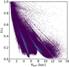 |
Fig. 1 Density distribution of the sample stars in the Rperi–ecc plane. A higher density is indicated by a lighter colour. |
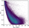 |
Fig. 2 Density distribution of the sample stars in the Rperi–ecc plane for an integration with a static axisymmetric potential (without the rotating bar). There is no trace of the overdensities seen in Fig. 1. |
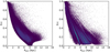 |
Fig. 3 Density distribution of the full sample in the Rperi–ecc plane computed from orbits generated with AGAMA. Left panel: the orbital parameters were recovered using the AGAMA built-in routine agama.potential.Rperiapo. Right panel: the orbital parameters were recovered directly from the orbital history of each tracer. |
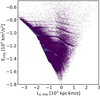 |
Fig. 4 Density distribution of the sample stars in the Lz,cha–Ez,cha plane. The diagonal overdensities seen in Fig. 1 appear as almost straight horizontal lines in prograde space (Lz,cha < 0) and turn at an angle when crossing into the retrograde region of space (Lz,cha > 0). |
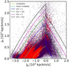 |
Fig. 5 Density distribution consisting of the stars from our full sample in the Jϕ–JR plane, the red points are the stars on the overdensities in Figs. 1 and 4, and the coloured solid lines are the theoretical predictions for the loci of the different resonances at specific values of the l/m ratio (see the legend). |
5 Interpretation of known substructures
Clustering of tracers in dynamical phase spaces is one of the premiere techniques for discovering and identifying substructures (whether in-situ or accreted merger remnants) among the MW stellar and globular cluster (GC) populations. Since the first systematic study by Massari et al. (2019) and many more recent works (i.e. Myeong et al. 2019; Koppelman et al. 2019a; Naidu et al. 2020; Horta et al. 2023; De Leo et al. 2026), this information has often been complemented with chemical analysis to provide classification for the MW stars and GCs (Horta et al. 2020; Callingham et al. 2022; Horta et al. 2023; Belokurov & Kravtsov 2024; Ceccarelli et al. 2024a; Bica et al. 2024; Ceccarelli et al. 2024b). We showed in the previous sections that resonant trapping induced by the rotating bar can produce overdensities of tracers in dynamical parameter spaces and can thus lead to a mistaken identification of substructures. Our findings agree well with the recent work of Woudenberg & Helmi (2025) and Dillamore & Sanders (2025), and our analysis highlights an easy and quick method to identify resonant loci directly in the orbital parameter spaces.
We investigated the stellar population of several MW substructures to confirm whether they might be partially or totally explained by bar-induced resonant trapping.
To do this, we ran ORBIT on the sample of stars attributed to many substructures identified as overdensities in phase space and tentatively attributed to relics of past merger events. Our analysis included the selection samples of some of the overdensities identified by Lövdal et al. (2022); Ruiz-Lara et al. (2022); Dodd et al. (2023) and the originally selected samples of candidate members for Nyx (Necib et al. 2020b), LMS-1 (Malhan et al. 2021), and Shakti and Shiva (Malhan & Rix 2024, and private communication from K. Malhan). When only coordinates and/or identifiers were provided, we crossmatched the catalogues with Gaia DR3 (Gaia Collaboration 2023b) and selected the stars with the usual Gaia quality cuts (Lindegren et al. 2021b). After correcting for the zero-point offset (Lindegren et al. 2021a), we obtained the distances for these samples by inversion of the Gaia parallaxes.
By determining roughly how many tracers of a given substructure lie on or near resonant loci, we gauged the degree of contamination of the substructure by resonances. For any given tracer, inhabiting a resonant orbit and belonging to a specific structure are not mutually exclusive conditions. The problem arises when a candidate structure is not easily distinguished from nearby or overlapping (in chemo-dynamical parameter spaces) structures, beside the fact of being an overdensity. In cases like this, it is important to determine how much of a density boost was due to resonant trapping and if the candidate structure would have been detected anyway without this contribution.
Fig. 7 shows the stellar distribution of the members identified in Dodd et al. (2023) of the thick disc (in cyan) and Gaia-Enceladus-Sausage (GES, Koppelman et al. 2018; Belokurov et al. 2018; Haywood et al. 2018; Helmi et al. 2018, in yellow), superimposed on our main sample on the Rperi–ecc plane. Given the large number of tracers belonging to the GES (which is thought to be the most massive accretion event of the MW) and to the disc, we were not surprised to find some of them on resonant loci (especially for the disc, as the orbits are prograde and more planar). Nonetheless, the tracers of both of these structures are spread around large regions of phase space (even more evident in Fig. 8) and have distinct and well-defined chemo-dynamical identities. The main result of applying our analysis to these structures is that we verified that it does not mistakenly identify all existing substructures as resonant trapping loci.
Moving on to smaller candidate merger events, we studied the relation with the resonances, if any, of the stellar populations of Nyx (Necib et al. 2020b,a, 2022), Thamnos (Koppelman et al. 2019a), Shakti and Shiva (Malhan & Rix 2024), LMS-1/Wukong (Naidu et al. 2020; Yuan et al. 2020), Cluster 3 (Lövdal et al. 2022; Ruiz-Lara et al. 2022) and the Helmi streams (Helmi et al. 1999; Koppelman et al. 2019b).
For Shiva, LMS-1/Wukong and the Helmi streams, our conservative selection found a small fraction (<10%) of stars on resonant orbits for each structure. For Cluster 3 (green points in Fig. 9) and Shakti (cyan points in the same figure) we found that 16.4% and 18.5%, respectively, of their member stars are on resonant orbits. Thamnos (yellow points in Fig. 9), the only purely retrograde structure we analysed, has no stars on resonant orbits according to our strict criteria. Finally, Nyx has the highest number of stars on resonant orbits, with 69.6%. As evidenced by the distribution of the Nyx stellar population in both Rperi–ecc (Fig. 10) and Lz,cha–Echa (Fig. 11) spaces, most of the stars are on or very close to the resonant loci.
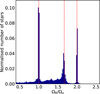 |
Fig. 6 Distribution of the orbital frequency ratios ΩR/Ωx for our full sample, the red dashed lines mark the resonant loci at ratios equal to 1, 5/3, and 2. |
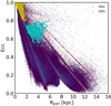 |
Fig. 7 Tracer distributions for thick disc (cyan stars) and GES (yellow circles), overlaid on our main sample (underlying colour map), in the Rperi–ecc plane. The dashed red lines identify the resonant trapping loci. |
 |
Fig. 8 Tracer distribution for the thick disc (cyan stars) and GES (yellow circles), overlaid on our main sample (underlying colour map), in the Lz,cha–Echa plane. The dashed red lines identify the resonant trapping loci. |
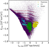 |
Fig. 9 Tracer distribution for Thamnos (yellow points), C3 (green points) and Shakti (cyan points), overlaid on our main sample (underlying colour map), in the Lz,cha–Echa plane. The dashed red lines identify the resonant trapping loci. |
6 Discussion
We have shown that the bar-induced resonances produce overdensities clearly visible in different parameter spaces, and these can be mistaken for genuine substructures of the MW. It is only natural to find a small fraction of stars within our selection of trapped stars, among the structures analysed, and particularly for those spanning a wide range of dynamical parameters. Even for smaller candidate merger events such as Shiva and LMS-1/Wukong, the limited contamination by stars that are trapped in resonances is not particularly concerning, given that their stars have been orbiting inside the MW potential for a very long time. The cases we are most interested in discussing are the structures that are contaminated to a higher degree. Their discovery might have been mainly driven by the enhanced clustering caused by resonance trapping.
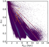 |
Fig. 10 Tracer distribution for Nyx (orange stars), overlaid on our main sample (underlying colour map), in the Rperi–ecc plane. The dashed red lines identify the resonant trapping loci. |
 |
Fig. 11 Tracer distribution for Nyx (orange stars), overlaid on our main sample (underlying colour map), in the Lz,cha–Echa plane. The dashed red lines identify the resonant trapping loci. |
6.1 Cluster 3
This structure (Lövdal et al. 2022; Ruiz-Lara et al. 2022) is located below the GES in the Lz–Etot plane with mixed dynamical signatures, and most of its member stars seem to have an in-situ chemistry. While we do not study the exact composition, characteristics, and ancestry of this group, we have to mention that the region of dynamical space it inhabits has been linked to the MW disc and some other in-situ populations (Aurora and Poor Old Heart Belokurov & Kravtsov 2022; Myeong et al. 2022; Rix et al. 2022). Regardless of the nature of Cluster 3, its detection has received a substantial boost from the density enhancement caused by stars trapped on resonances. To be sure of the robustness of our result, we repeated the analysis for Cluster 3 stars by taking the observational errors into account. For each member star, we produced 100 “clones” with the 6D information extracted from Gaussian distributions having the observed value of each parameter as the mean of this distribution and the observational uncertainties as the standard deviation. In this expanded sample of Cluster 3 stars, we found that 16.8% of them were trapped by resonances, confirming our first estimate.
6.2 Shakti
Of the two candidate merger events identified by Malhan & Rix (2024), Shakti (the least bound and more energetic relic in the original paper) seems to be contaminated by stars trapped near the corotation resonance. As done for Cluster 3 in Sect. 6.1, we repeated our analysis by taking observational errors into account and found that 17.7% of the population is trapped, in line with our first result. These resonant stars populate a very dense clump of Shakti’s tracers just below Echa = −1.2 × 10⁵ km2/s2 (clearly visible in Fig. 9) and we question whether without this substantial density enhancement, the structure would have been identified. Considering that the chemical properties of Shakti are compatible with the in-situ (disc) population and the loci in dynamical space inhabited by its tracers overlap almost completely with the disc, we are inclined to agree with the in-situ (disc) origin hypothesis proposed by Malhan & Rix (2024), which is supported by the literature (Myeong et al. 2018; Dillamore et al. 2024b).
6.3 Nyx
Most of Nyx members stars trapped on the OLR (l/m = 1/2) and l/m = 1 resonances, and it therefore appears clear that Nyx is no genuine merger event of the MW but rather a structure caused by resonant trapping. To ensure that such a strong claim is robust, we repeated the analysis for the Nyx stars by taking the observational errors into account, as done in the previous cases. We found that 66.9% of the expanded Nyx sample lies on trapped orbits, which shows that even when the observational uncertainties are accounted for, the Nyx population is not freed from the resonances. The visual inspection of the stellar orbits for Nyx members is the final confirmation that they are trapped in resonant loci (Fig. 12). Looking at the chemical evidence available for Nyx stars, recent studies have found disc-like abundance patterns. Horta et al. (2023), examined a sample of APOGEE (Majewski et al. 2017) stars, and found that abundance distributions of the α elements of Nyx members strongly overlaps with the high-α thick disc. Likewise, Wang et al. (2023) used high-resolution spectroscopic data from Keck/HIRES (Vogt et al. 1994) and Magellan/MIKE (Bernstein et al. 2003) and concluded that the chemical abundances of Nyx members are consistent with those of the high-α thick disc. These chemical studies put into question Nyx as an independent structure and further strengthen our conclusion that Nyx is an overdensity caused by resonant trapping and not a “bona fide” merger event.
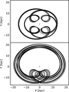 |
Fig. 12 Two orbits of Nyx stars (in black, representative of the whole sample) on the XY plane in the reference frame corotating with the bar. The red star marks the Galactic centre. The stars are clearly trapped in resonance. |
6.4 A retrograde outlier: Thamnos
The only purely retrograde structure we analysed, Thamnos, appears to be substantially untouched by resonant trapping (only one star out of 851 passed our threefold criteria, i.e. 0.12% of the sample). This seems to run counter to what is shown in Fig. 9 where the highest Echa ridge of Thamnos tracers (the yellow points) appears to be detached from the rest of the population, sitting on top of the resonance locus around the area of Echa ≃ −1.2 × 10⁵ km2/s2 and Lz,cha ≃ 103 kpc km/s. Because the resonance loci in the retrograde region (Lz ≡ Jϕ > 0) always appear to take a different geometry than what is seen in the prograde region (i.e. Figures 4 and 5), we only selected the retrograde stars in our sample and determined whether the resonant loci in Rperi–ecc appeared to be different from what we found before (Fig. 1). While this retrograde sample is much smaller, with <20 000 stars, it nonetheless allowed us to identify two retrograde resonant loci that are distinct from those identified previously in the full sample (completely dominated by the prograde population). Fig. 13 shows the distribution in Rperi–ecc space of the retrograde stars in our sample. Clearly, no resonant track is aligned with the dashed red line (the first resonant locus identified in Fig. 1), but a new track lies quasi-parallel to the dashed red line on its right.
We parametrised the retrograde resonant loci (see Appendix C) and repeated our analysis for Thamnos, identifying 8.5% of its members as trapped around the l/m = 3/2 resonance. When the observational errors are taken into account with the same method used for the other structures, 8.2% of the extended sample are trapped in resonance, confirming our result. While the portion of Thamnos stars in resonance is quite small, the peculiarity is that it is composed entirely of the stars at the highest energies. Going back to the original identification of this structure, our analysis suggests that “Thamnos 1” (the most energetic of the two clumps contributing to the structure in Koppelman et al. 2019a) might be an overdensity mostly populated by trapped stars. Considering the mounting evidence that Thamnos is heavily contaminated by both in-situ and GES tracers (Ruiz-Lara et al. 2022; Dodd et al. 2025; Ceccarelli et al. 2025), it is important to explore possible alternative explanations for the origin of the stellar population that appears to inhabit this structure and resonant trapping seems to be able to explain the high-energy population.
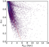 |
Fig. 13 Density distribution of the retrograde stars of the sample in the Rperi–ecc space. The dashed red line sits on top of the first resonant locus identified in Fig. 1 and is clearly different from the quasi-parallel line of the retrograde locus visible on its right. |
7 Conclusions
We have shown that fully accounting for the effect of the bar during the recovery of the orbital parameters allows us to identify the loci of bar-induced resonances in different orbital parameter spaces. The tracers trapped on resonances clearly cluster in conspicuous overdensities that are easily identifiable, especially in Rperi–ecc. This unlocks an efficient and fast way of identifying tracers that are trapped on resonant orbits already in the space of the orbital parameters (Rperi, Rapo, and ecc) without the need to transition into action space. This transition required several theoretical assumptions and approximations (because regular orbits are extremely rare in real data) that are thus avoided, allowing a precise identification of resonances in any potential.
Furthermore, overdensities of tracers that are generated by the bar-induced resonances and overdensities due to past merger are indistinguishable for clustering algorithms, with the chance of a mistaken identification of candidate merger events. We showed that structures that were previously identified as mergers of the MW, can be constituted partially or totally by stars on resonant orbits. In particular, Cluster 3 and Shakti seem to have received a substantial density enhancement from resonant trapping, while Nyx proves to be an exemplary case of an overdensity that is not a real merger event, but is instead caused by stars trapped on resonances. The only purely retrograde structure we analysed, Thamnos, also shows signs of contamination from resonance-trapped stars, which affects its highest energy members (“Thamnos 1”).
As discussed in Sect. 4, the available theoretical framework for the calculation of resonant loci is developed in action space and only offers an approximation of the real, complex situation of the MW. While we showed the robustness of our empirical method for the identification of resonant structures, we also need to point out the lack of precise theoretical (whether analytical or numerical) predictions of the resonant loci in the dynamical spaces of the orbital parameters.
Data availability
The data underlying this article come from public sources listed in Section 2. The results derived from ORBIT will be made available upon reasonable request.
Acknowledgements
The authors would like to thank the anonymous referee for insightful comments that helped improve and clarify the manuscript. The authors would also like to thank to E. Ceccarelli and E. Dodd for valuable discussions. MDL and AM acknowledge financial support from the project “LEGO − Reconstructing the building blocks of the Galaxy by chemical tagging” (PI: Mucciarelli) granted by the Italian MUR through contract PRIN2022LLP8TK_001. BA-T acknowledges support from the ANID Doctoral Fellowship through grant number 21231305. This research made use of the Astropy (Astropy Collaboration 2013, 2018), Matplotlib (Hunter 2007) and Numpy (Harris et al. 2020) packages.
References
- Astropy Collaboration (Robitaille, T. P., et al.) 2013, A&A, 558, A33 [NASA ADS] [CrossRef] [EDP Sciences] [Google Scholar]
- Astropy Collaboration (Price-Whelan, A. M., et al.) 2018, AJ, 156, 123 [Google Scholar]
- Atkinson, K. E. 1991, An Introduction to Numerical Analysis, 2nd edn. (John Wiley & Sons) [Google Scholar]
- Belokurov, V., & Kravtsov, A. 2022, MNRAS, 514, 689 [NASA ADS] [CrossRef] [Google Scholar]
- Belokurov, V., & Kravtsov, A. 2024, MNRAS, 528, 3198 [CrossRef] [Google Scholar]
- Belokurov, V., Erkal, D., Evans, N. W., Koposov, S. E., & Deason, A. J. 2018, mnras, 478, 611 [Google Scholar]
- Bellazzini, M., Massari, D., De Angeli, F., et al. 2023a, A&A, 674, A194 [NASA ADS] [CrossRef] [EDP Sciences] [Google Scholar]
- Bellazzini, M., Massari, D., de Angeli, F., et al. 2023b, VizieR Online Data Catalog: Galactic giant stars photometric metallicity (Bellazzini+, 2023), VizieR On-line Data Catalog: J/A+A/674/A194. Originally published in: 2023A&A...674A.194B [Google Scholar]
- Bernstein, R., Shectman, S. A., Gunnels, S. M., Mochnacki, S., & Athey, A. E. 2003, SPIE Conf. Ser., 4841, 1694 [NASA ADS] [Google Scholar]
- Bica, E., Ortolani, S., Barbuy, B., & Oliveira, R. A. P. 2024, A&A, 687, A201 [NASA ADS] [CrossRef] [EDP Sciences] [Google Scholar]
- Binney, J., & Tremaine, S. 2008, Galactic Dynamics, 2nd edn. (Princeton University Press) [Google Scholar]
- Binney, J., Gerhard, O., & Spergel, D. 1997, MNRAS, 288, 365 [NASA ADS] [CrossRef] [Google Scholar]
- Bovy, J. 2015, ApJS, 216, 29 [NASA ADS] [CrossRef] [Google Scholar]
- Callingham, T. M., Cautun, M., Deason, A. J., et al. 2022, MNRAS, 513, 4107 [NASA ADS] [CrossRef] [Google Scholar]
- Ceccarelli, E., Massari, D., Mucciarelli, A., et al. 2024a, A&A, 684, A37 [NASA ADS] [CrossRef] [EDP Sciences] [Google Scholar]
- Ceccarelli, E., Mucciarelli, A., Massari, D., Bellazzini, M., & Matsuno, T. 2024b, A&A, 691, A226 [NASA ADS] [CrossRef] [EDP Sciences] [Google Scholar]
- Ceccarelli, E., Massari, D., Palla, M., et al. 2025, A&A, 704, A180 [NASA ADS] [CrossRef] [EDP Sciences] [Google Scholar]
- Chiba, R., & Schönrich, R. 2021, MNRAS, 505, 2412 [NASA ADS] [CrossRef] [Google Scholar]
- Chiba, R., Friske, J. K. S., & Schönrich, R. 2021, MNRAS, 500, 4710 [Google Scholar]
- Contopoulos, G. 1970, ApJ, 160, 113 [Google Scholar]
- De Leo, M., Zoccali, M., Olivares-Carvajal, J., et al. 2026, A&A, 706, A130 [NASA ADS] [CrossRef] [EDP Sciences] [Google Scholar]
- Debattista, V. P., & Sellwood, J. A. 1998, ApJ, 493, L5 [Google Scholar]
- Debattista, V. P., & Sellwood, J. A. 2000, ApJ, 543, 704 [Google Scholar]
- Dehnen, W. 2000, AJ, 119, 800 [NASA ADS] [CrossRef] [Google Scholar]
- Dillamore, A. M., & Sanders, J. L. 2025, MNRAS, 542, 1331 [Google Scholar]
- Dillamore, A. M., Belokurov, V., Evans, N. W., & Davies, E. Y. 2023, MNRAS, 524, 3596 [NASA ADS] [CrossRef] [Google Scholar]
- Dillamore, A. M., Belokurov, V., & Evans, N. W. 2024a, MNRAS, 532, 4389 [NASA ADS] [CrossRef] [Google Scholar]
- Dillamore, A. M., Monty, S., Belokurov, V., & Evans, N. W. 2024b, ApJ, 971, L4 [Google Scholar]
- Dodd, E., Callingham, T. M., Helmi, A., et al. 2023, A&A, 670, L2 [NASA ADS] [CrossRef] [EDP Sciences] [Google Scholar]
- Dodd, E., Ruiz-Lara, T., Helmi, A., et al. 2025, A&A, 698, A277 [NASA ADS] [CrossRef] [EDP Sciences] [Google Scholar]
- D’Onghia, E., & Aguerri, L. J. A. 2020, ApJ, 890, 117 [CrossRef] [Google Scholar]
- Dumas, H. S., & Laskar, J. 1993, Phys. Rev. Lett., 70, 2975 [NASA ADS] [CrossRef] [Google Scholar]
- Earn, D. J. D., & Lynden-Bell, D. 1996, MNRAS, 278, 395 [Google Scholar]
- Eggen, O. J. 1958, MNRAS, 118, 154 [NASA ADS] [Google Scholar]
- Evans, N. W., de Zeeuw, P. T., & Lynden-Bell, D. 1990, MNRAS, 244, 111 [Google Scholar]
- Gaia Collaboration (Brown, A. G. A., et al.) 2016, A&A, 595, A2 [NASA ADS] [CrossRef] [EDP Sciences] [Google Scholar]
- Gaia Collaboration (Montegriffo, P., et al.) 2023a, A&A, 674, A33 [CrossRef] [EDP Sciences] [Google Scholar]
- Gaia Collaboration (Vallenari, A., et al.) 2023b, A&A, 674, A1 [NASA ADS] [CrossRef] [EDP Sciences] [Google Scholar]
- GRAVITY Collaboration (Abuter, R., et al.) 2019, A&A, 625, L10 [NASA ADS] [CrossRef] [EDP Sciences] [Google Scholar]
- Hairer, E., Lubich, C., & Wanner, G. 2003, Acta Numer., 12, 399 [CrossRef] [MathSciNet] [Google Scholar]
- Harris, C. R., Millman, K. J., van der Walt, S. J., et al. 2020, Nature, 585, 357 [NASA ADS] [CrossRef] [Google Scholar]
- Harsoula, M., & Kalapotharakos, C. 2009, MNRAS, 394, 1605 [NASA ADS] [CrossRef] [Google Scholar]
- Haywood, M., Di Matteo, P., Lehnert, M. D., et al. 2018, ApJ, 863, 113 [Google Scholar]
- Helmi, A., & de Zeeuw, P. T. 2000, MNRAS, 319, 657 [Google Scholar]
- Helmi, A., White, S. D. M., de Zeeuw, P. T., & Zhao, H. 1999, Nature, 402, 53 [Google Scholar]
- Helmi, A., Babusiaux, C., Koppelman, H. H., et al. 2018, Nature, 563, 85 [Google Scholar]
- Henon, M. 1959, Ann. Astrophys., 22, 126 [NASA ADS] [Google Scholar]
- Horta, D., Schiavon, R. P., Mackereth, J. T., et al. 2020, MNRAS, 493, 3363 [NASA ADS] [CrossRef] [Google Scholar]
- Horta, D., Schiavon, R. P., Mackereth, J. T., et al. 2023, MNRAS, 520, 5671 [NASA ADS] [CrossRef] [Google Scholar]
- Hunter, J. D. 2007, Comput. Sci. Eng., 9, 90 [NASA ADS] [CrossRef] [Google Scholar]
- Hunter, G. H., Sormani, M. C., Beckmann, J. P., et al. 2024, A&A, 692, A216 [NASA ADS] [CrossRef] [EDP Sciences] [Google Scholar]
- Kalnajs, A. J. 1991, in Dynamics of Disc Galaxies, ed. B. Sundelius, 323 [Google Scholar]
- Khoperskov, S., & Gerhard, O. 2022, A&A, 663, A38 [NASA ADS] [CrossRef] [EDP Sciences] [Google Scholar]
- Khoperskov, S., Gerhard, O., Di Matteo, P., et al. 2020, A&A, 634, L8 [NASA ADS] [CrossRef] [EDP Sciences] [Google Scholar]
- Koppelman, H., Helmi, A., & Veljanoski, J. 2018, ApJ, 860, L11 [NASA ADS] [CrossRef] [Google Scholar]
- Koppelman, H. H., Helmi, A., Massari, D., Price-Whelan, A. M., & Starkenburg, T. K. 2019a, A&A, 631, L9 [NASA ADS] [CrossRef] [EDP Sciences] [Google Scholar]
- Koppelman, H. H., Helmi, A., Massari, D., Roelenga, S., & Bastian, U. 2019b, A&A, 625, A5 [NASA ADS] [CrossRef] [EDP Sciences] [Google Scholar]
- Laskar, J. 1990, Icarus, 88, 266 [NASA ADS] [CrossRef] [Google Scholar]
- Lian, J., Zasowski, G., Mackereth, T., et al. 2022, MNRAS, 513, 4130 [NASA ADS] [CrossRef] [Google Scholar]
- Lin, C. C., & Shu, F. H. 1964, ApJ, 140, 646 [Google Scholar]
- Lin, C. C., & Shu, F. H. 1966, Proc. Natl. Acad. Sci., 55, 229 [NASA ADS] [CrossRef] [Google Scholar]
- Lindblad, B. 1961, Stockholms Observatoriums Ann., 8, 8 [Google Scholar]
- Lindblad, B., & Langebartel, R. G. 1953, Stockholms Observatoriums Ann., 17, 6 [Google Scholar]
- Lindegren, L., Bastian, U., Biermann, M., et al. 2021a, A&A, 649, A4 [EDP Sciences] [Google Scholar]
- Lindegren, L., Klioner, S. A., Hernández, J., et al. 2021b, A&A, 649, A2 [EDP Sciences] [Google Scholar]
- Liu, H., Du, C., Ye, D., Zhang, J., & Deng, M. 2024, ApJ, 976, 161 [Google Scholar]
- Long, K., & Murali, C. 1992, ApJ, 397, 44 [NASA ADS] [CrossRef] [Google Scholar]
- Lövdal, S. S., Ruiz-Lara, T., Koppelman, H. H., et al. 2022, A&A, 665, A57 [NASA ADS] [CrossRef] [EDP Sciences] [Google Scholar]
- Lynden-Bell, D. 1979, MNRAS, 187, 101 [Google Scholar]
- Majewski, S. R., Schiavon, R. P., Frinchaboy, P. M., et al. 2017, AJ, 154, 94 [NASA ADS] [CrossRef] [Google Scholar]
- Malhan, K., & Rix, H.-W. 2024, ApJ, 964, 104 [NASA ADS] [CrossRef] [Google Scholar]
- Malhan, K., Yuan, Z., Ibata, R. A., et al. 2021, ApJ, 920, 51 [NASA ADS] [CrossRef] [Google Scholar]
- Massari, D., Koppelman, H. H., & Helmi, A. 2019, A&A, 630, L4 [NASA ADS] [CrossRef] [EDP Sciences] [Google Scholar]
- McKee, C. F., Parravano, A., & Hollenbach, D. J. 2015, ApJ, 814, 13 [Google Scholar]
- McMillan, P. J. 2013, MNRAS, 430, 3276 [NASA ADS] [CrossRef] [Google Scholar]
- McMillan, P. J. 2017, MNRAS, 465, 76 [NASA ADS] [CrossRef] [Google Scholar]
- Miyamoto, M., & Nagai, R. 1975, PASJ, 27, 533 [NASA ADS] [Google Scholar]
- Moreno, E., Pichardo, B., & Schuster, W. J. 2015, MNRAS, 451, 705 [NASA ADS] [CrossRef] [Google Scholar]
- Moreno, E., Fernández-Trincado, J. G., Schuster, W. J., Pérez-Villegas, A., & Chaves-Velasquez, L. 2021, MNRAS, 506, 4687 [CrossRef] [Google Scholar]
- Myeong, G. C., Evans, N. W., Belokurov, V., Sanders, J. L., & Koposov, S. E. 2018, ApJ, 856, L26 [NASA ADS] [CrossRef] [Google Scholar]
- Myeong, G. C., Vasiliev, E., Iorio, G., Evans, N. W., & Belokurov, V. 2019, MNRAS, 488, 1235 [Google Scholar]
- Myeong, G. C., Belokurov, V., Aguado, D. S., et al. 2022, ApJ, 938, 21 [NASA ADS] [CrossRef] [Google Scholar]
- Naidu, R. P., Conroy, C., Bonaca, A., et al. 2020, ApJ, 901, 48 [Google Scholar]
- Navarro, J. F., Frenk, C. S., & White, S. D. M. 1996, ApJ, 462, 563 [Google Scholar]
- Necib, L., Ostdiek, B., Lisanti, M., et al. 2020a, ApJ, 903, 25 [NASA ADS] [CrossRef] [Google Scholar]
- Necib, L., Ostdiek, B., Lisanti, M., et al. 2020b, Nat. Astron., 4, 1078 [NASA ADS] [CrossRef] [Google Scholar]
- Necib, L., Ostdiek, B., Lisanti, M., et al. 2022, Nat. Astron., 6, 866 [Google Scholar]
- Pérez-Villegas, A., Portail, M., Wegg, C., & Gerhard, O. 2017, ApJ, 840, L2 [Google Scholar]
- Plummer, H. C. 1911, MNRAS, 71, 460 [Google Scholar]
- Portail, M., Wegg, C., & Gerhard, O. 2015, MNRAS, 450, L66 [NASA ADS] [CrossRef] [Google Scholar]
- Portail, M., Gerhard, O., Wegg, C., & Ness, M. 2017, MNRAS, 465, 1621 [NASA ADS] [CrossRef] [Google Scholar]
- Price-Whelan, A. M. 2015, SuperFreq: Numerical determination of fundamental frequencies of an orbit, Astrophysics Source Code Library [record ascl:1511.001] [Google Scholar]
- Queiroz, A. B. A., Chiappini, C., Perez-Villegas, A., et al. 2021, A&A, 656, A156 [NASA ADS] [CrossRef] [EDP Sciences] [Google Scholar]
- Rix, H.-W., Chandra, V., Andrae, R., et al. 2022, ApJ, 941, 45 [NASA ADS] [CrossRef] [Google Scholar]
- Roberts, J. A. G., & Quispel, G. R. W. 1992, Phys. Rep., 216, 63 [Google Scholar]
- Ruiz-Lara, T., Matsuno, T., Lövdal, S. S., et al. 2022, A&A, 665, A58 [NASA ADS] [CrossRef] [EDP Sciences] [Google Scholar]
- Sanders, J. L., Smith, L., & Evans, N. W. 2019, MNRAS, 488, 4552 [NASA ADS] [CrossRef] [Google Scholar]
- Schönrich, R., Binney, J., & Dehnen, W. 2010, MNRAS, 403, 1829 [NASA ADS] [CrossRef] [Google Scholar]
- Sormani, M. C., Gerhard, O., Portail, M., Vasiliev, E., & Clarke, J. 2022, MNRAS, 514, L1 [NASA ADS] [CrossRef] [Google Scholar]
- Valenti, E., Zoccali, M., Gonzalez, O. A., et al. 2016, A&A, 587, L6 [NASA ADS] [CrossRef] [EDP Sciences] [Google Scholar]
- Vasiliev, E. 2019, MNRAS, 482, 1525 [Google Scholar]
- Verlet, L. 1967, Phys. Rev., 159, 98 [CrossRef] [Google Scholar]
- Vogt, S. S., Allen, S. L., Bigelow, B. C., et al. 1994, SPIE Conf. Ser., 2198, 362 [NASA ADS] [Google Scholar]
- Wang, S., Necib, L., Ji, A. P., et al. 2023, ApJ, 955, 129 [NASA ADS] [CrossRef] [Google Scholar]
- Wegg, C., Gerhard, O., & Portail, M. 2015, MNRAS, 450, 4050 [NASA ADS] [CrossRef] [Google Scholar]
- Woudenberg, H. C., & Helmi, A. 2025, A&A, 700, A240 [NASA ADS] [CrossRef] [EDP Sciences] [Google Scholar]
- Yuan, Z., Chang, J., Beers, T. C., & Huang, Y. 2020, ApJ, 898, L37 [Google Scholar]
- Zoccali, M., Valenti, E., & Gonzalez, O. A. 2018, A&A, 618, A147 [NASA ADS] [CrossRef] [EDP Sciences] [Google Scholar]
Appendix A Comparison of radial action recovery
As a sanity check for our numerical method of recovery of the radial action JR, we compare our results with those derived for the same sample in Bellazzini et al. (2023a) using a McMillan (2017) potential and the AGAMA action finder built-in routines using the Stäckel approximation (see the AGAMA reference documentation). Fig. A.1 shows the reasonable agreement of the two different estimations of JR despite the different methods and underlying potentials used.
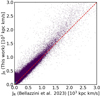 |
Fig. A.1 Comparison of the JR recovered in Bellazzini et al. (2023a) and in this work, the dashed red line is the equivalence line. |
Appendix B Effect of changes in the pattern speed
To test the robustness of our method against changes in the pattern speed of the bar, the parameter affecting the resonances the most, we repeated the entire analysis setting Ωp = 35 km s−1 kpc−1. We reran ORBIT on the entire sample, and were able to identify the resonance loci in Rperi − ecc and Lz,cha − Echa. As mentioned in Sec 4, the loci are slightly moved with respect to the integration at Ωp = 41.3 km s−1 kpc−1, used throughout the main text. In order to fully test the robustness of our results, we repeated the analysis of the Nyx sample, the most important finding of this work. Figures B.1 and B.2 show the outcome of this test, with 62.3% of the Nyx member stars ending on the resonant loci. To further prove the robustness of our method and results, we repeated our analysis for the main sample and Nyx members with Ωp = 45 km s−1 kpc−1. Again, we were able to identify the resonant loci and show that the majority of Nyx tracers (43 out of 69) are trapped in them (Figures B.3 and B.4).
Appendix C Selection of resonant loci
The resonant loci in Rperi–ecc and Lz,cha–Echa are identified by the equations reported below and are shown in the Fig. C.1 and C.3. In Rperi–ecc space the resonant loci are parametrised as follows (with the Rperi in kpc):
ecc = 0.97 − 0.166 · Rperi for 0.6 ≤ Rperi ≤ 5.6
ecc = 1.00 − 0.106 · Rperi for 0.6 ≤ Rperi ≤ 7.5
ecc = 0.8675 − 0.0875 · Rperi for 7.5 ≤ Rperi ≤ 9.2
ecc = 1.020 − 0.0795 · Rperi for 0.6 ≤ Rperi ≤ 12.5
ecc = 1.046 − 0.0645 · Rperi for 0.6 ≤ Rperi ≤ 13.5
The intervals marked by the red dashed lines in Fig. C.1 are obtained by adding to the equation of each locus reported above an offset equal to the tolerances specified in Sect. 4: ±0.03, ±0.02, ±0.02, ±0.015 and ±0.01.
As explained in Sect. 6.4, the resonant loci in the retrograde region are different and are parametrised as follows:
ecc = 1.042 − 0.171 · Rperi for 0.6 ≤ Rperi ≤ 6.0
ecc = 1.055 − 0.1165 · Rperi for 0.6 ≤ Rperi ≤ 9.0
The intervals in Fig. C.2 are obtained by adding offsets of, respectively, ±0.015, and ±0.01.
In Lz,cha–Echa space the resonant loci are parametrised as follows (with Lz,cha in 103 kpc km/s and Echa in 105 km2/s2):
Echa = −1.303 − 0.029 · Lz,cha for −1.48 ≤ Lz,cha ≤ −0.75
Echa = −1.355 − 0.1 · Lz,cha for −0.75 ≤ Lz,cha ≤ −0.25
Echa = −1.393 − 0.25 · Lz,cha for −0.25 ≤ Lz,cha ≤ −0.15
Echa = −1.4275 − 0.50 · Lz,cha for −0.25 ≤ Lz,cha ≤ 0.3
Echa = −1.065 − 0.015 · Lz,cha for −2.1 ≤ Lz,cha ≤ 0.29
Echa = −1.10 − 0.135 · Lz,cha for −0.29 ≤ Lz,cha ≤ 0.5
Echa = −1.14 − 0.06 · Lz,cha for 0.5 ≤ Lz,cha ≤ 1.4
Echa = −0.925 − 0.007 · Lz,cha for −2.6 ≤ Lz,cha ≤ −0.28
Echa = −0.945 − 0.075 · Lz,cha for −0.28 ≤ Lz,cha ≤ 0.75
Echa = −0.8275 − 0.0015 · Lz,cha for −3.1 ≤ Lz,cha ≤ −0.28
Echa = −0.845 − 0.053 · Lz,cha for −0.28 ≤ Lz,cha ≤ 0.75
The offset needed to reproduce the intervals in Fig. C.3 is ±0.01 105 km2/s2.
 |
Fig. C.1 Density distribution of the full sample in Rperi–ecc, the red dahsed lines are the confines of the selections boxes for the resonant loci. |
All Tables
All Figures
|
Fig. 1 Density distribution of the sample stars in the Rperi–ecc plane. A higher density is indicated by a lighter colour. |
| In the text | |
|
Fig. 2 Density distribution of the sample stars in the Rperi–ecc plane for an integration with a static axisymmetric potential (without the rotating bar). There is no trace of the overdensities seen in Fig. 1. |
| In the text | |
|
Fig. 3 Density distribution of the full sample in the Rperi–ecc plane computed from orbits generated with AGAMA. Left panel: the orbital parameters were recovered using the AGAMA built-in routine agama.potential.Rperiapo. Right panel: the orbital parameters were recovered directly from the orbital history of each tracer. |
| In the text | |
|
Fig. 4 Density distribution of the sample stars in the Lz,cha–Ez,cha plane. The diagonal overdensities seen in Fig. 1 appear as almost straight horizontal lines in prograde space (Lz,cha < 0) and turn at an angle when crossing into the retrograde region of space (Lz,cha > 0). |
| In the text | |
|
Fig. 5 Density distribution consisting of the stars from our full sample in the Jϕ–JR plane, the red points are the stars on the overdensities in Figs. 1 and 4, and the coloured solid lines are the theoretical predictions for the loci of the different resonances at specific values of the l/m ratio (see the legend). |
| In the text | |
|
Fig. 6 Distribution of the orbital frequency ratios ΩR/Ωx for our full sample, the red dashed lines mark the resonant loci at ratios equal to 1, 5/3, and 2. |
| In the text | |
|
Fig. 7 Tracer distributions for thick disc (cyan stars) and GES (yellow circles), overlaid on our main sample (underlying colour map), in the Rperi–ecc plane. The dashed red lines identify the resonant trapping loci. |
| In the text | |
|
Fig. 8 Tracer distribution for the thick disc (cyan stars) and GES (yellow circles), overlaid on our main sample (underlying colour map), in the Lz,cha–Echa plane. The dashed red lines identify the resonant trapping loci. |
| In the text | |
|
Fig. 9 Tracer distribution for Thamnos (yellow points), C3 (green points) and Shakti (cyan points), overlaid on our main sample (underlying colour map), in the Lz,cha–Echa plane. The dashed red lines identify the resonant trapping loci. |
| In the text | |
|
Fig. 10 Tracer distribution for Nyx (orange stars), overlaid on our main sample (underlying colour map), in the Rperi–ecc plane. The dashed red lines identify the resonant trapping loci. |
| In the text | |
|
Fig. 11 Tracer distribution for Nyx (orange stars), overlaid on our main sample (underlying colour map), in the Lz,cha–Echa plane. The dashed red lines identify the resonant trapping loci. |
| In the text | |
|
Fig. 12 Two orbits of Nyx stars (in black, representative of the whole sample) on the XY plane in the reference frame corotating with the bar. The red star marks the Galactic centre. The stars are clearly trapped in resonance. |
| In the text | |
|
Fig. 13 Density distribution of the retrograde stars of the sample in the Rperi–ecc space. The dashed red line sits on top of the first resonant locus identified in Fig. 1 and is clearly different from the quasi-parallel line of the retrograde locus visible on its right. |
| In the text | |
|
Fig. A.1 Comparison of the JR recovered in Bellazzini et al. (2023a) and in this work, the dashed red line is the equivalence line. |
| In the text | |
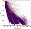 |
Fig. B.1 Same as Fig. 10 but for Ωp = 35 km s−1 kpc−1. |
| In the text | |
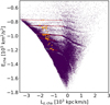 |
Fig. B.2 Same as Fig. 11 but for Ωp = 35 km s−1 kpc−1. |
| In the text | |
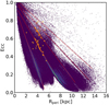 |
Fig. B.3 Same as Fig. 10 but for Ωp = 45 km s−1 kpc−1. |
| In the text | |
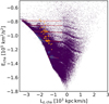 |
Fig. B.4 Same as Fig. 11 but for Ωp = 45 km s−1 kpc−1. |
| In the text | |
|
Fig. C.1 Density distribution of the full sample in Rperi–ecc, the red dahsed lines are the confines of the selections boxes for the resonant loci. |
| In the text | |
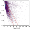 |
Fig. C.2 As Fig. C.1 but for the retrograde stars in the sample. |
| In the text | |
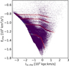 |
Fig. C.3 As Fig. C.1 but in Lz,cha–Echa space. |
| In the text | |
Current usage metrics show cumulative count of Article Views (full-text article views including HTML views, PDF and ePub downloads, according to the available data) and Abstracts Views on Vision4Press platform.
Data correspond to usage on the plateform after 2015. The current usage metrics is available 48-96 hours after online publication and is updated daily on week days.
Initial download of the metrics may take a while.