| Issue |
A&A
Volume 707, March 2026
|
|
|---|---|---|
| Article Number | A206 | |
| Number of page(s) | 19 | |
| Section | Numerical methods and codes | |
| DOI | https://doi.org/10.1051/0004-6361/202556748 | |
| Published online | 13 March 2026 | |
Automated model selection for the spectral fitting of large samples of active galactic nucleus spectra
1
Instituto de Física y Astronomía, Universidad de Valparaíso,
Gran Bretaña 1111,
Valparaíso,
Chile
2
Millennium Nucleus on Transversal Research and Technology to Explore Supermassive Black Holes (TITANS),
Chile
3
European Southern Observatory,
Karl-Schwarzschild-Str. 2,
85748
Garching,
Germany
4
Instituto de Alta Investigación, Universidad de Tarapacá,
Casilla 7D,
Arica,
Chile
5
Departamento de Astronomía, Universidad de Chile,
Camino el Observatorio 1515,
Santiago,
Chile
6
Astronomy Department, Universidad de Concepción,
Barrio Universitario S/N,
Concepción
4030000,
Chile
7
Millennium Institute of Astrophysics (MAS),
Nuncio Monseñor Sótero Sanz 100,
Providencia,
Santiago,
Chile
8
Kapteyn Astronomical Institute, University of Groningen,
9700 AV
Groningen,
The Netherlands
★ Corresponding author: This email address is being protected from spambots. You need JavaScript enabled to view it.
Received:
4
August
2025
Accepted:
29
January
2026
Abstract
Aims. We developed an algorithm to automatically recommend and selected the best model to fit active galactic nucleus (AGN) spectra in the ultraviolet/optical wavelength range, enhancing the efficiency of fitting large samples of AGN spectra by replacing the visual inspection and manual selection of the best model.
Methods. We employed the Penalized PiXel-Fitting (pPXF) software to fit AGN spectra using a complete model that includes: narrow and broad emission lines (NELs and BELs), Balmer continuum, Balmer high-order emission lines (H8-H50), FeII pseudo-continuum, AGN continuum, and stellar populations for objects with z < 1; we call this model-1. The fit residuals were analyzed using the discrete wavelet transform (DWT), looking for deviations in the DWT coefficients above some empirically determined threshold value. When deviations were detected in regions of interest of a spectrum (i.e., around Hα, Hβ, MgII, CIV, and [OIII]λ4959, 5007), the significance of the residuals and kinematics were used to recommend (or not) the addition of an extra fitting component for the model. When a new model is recommended, we compared the new fit and the previous one using the root-mean-square (RMS) difference and F-test. The final results of the developed algorithm are the selection of the best-fit model and the corresponding fit results. We validated the results of the algorithm using a sample of 800 SDSS AGN spectra. Each object was fitted using model-1 and the results were visually inspected by three human validators. The validators also recommended (or not) the addition of the same additional components that the algorithm is equipped to recommend.
Results. Comparing the recommendation of each validator and the algorithm, the median coincidence fraction is 0.83-0.88 for different threshold values. These values are comparable to the median coincidence fraction of 0.90 between human validators. The computational time of the model recommendation routine was <1s for 90 percent of the objects, compared to ≈60 s for visual inspection during the validation exercise.
Conclusions. The presented algorithm is an efficient and effective tool for the spectral fitting of large samples of AGN spectra with options for improvement and applications for specific studies.
Key words: methods: data analysis / techniques: spectroscopic / galaxies: active
© The Authors 2026
 Open Access article, published by EDP Sciences, under the terms of the Creative Commons Attribution License (https://creativecommons.org/licenses/by/4.0), which permits unrestricted use, distribution, and reproduction in any medium, provided the original work is properly cited.
This article is published in open access under the Subscribe to Open model. This email address is being protected from spambots. You need JavaScript enabled to view it. to support open access publication.
1 Introduction
Since the discovery of the first quasar (QSO) in 1963 (Schmidt 1963), the study of these objects has faced challenges due to their complex characteristics and behaviors. Despite the widespread adoption of the unified model to explain most active galactic nucleus (AGN) observations (Antonucci 1993) and the systematic characterization of the AGN spectra (Boroson & Green 1992); Sulentic et al. 2000; Marziani et al. 2018), a more complete census of the AGNs remains essential. Properties attributed exclusively to AGNs can be identified when observed with specific techniques such as X-ray or ultraviolet/optical (UV/optical) spectroscopy. In the UV/optical spectral range, the presence of broad emission lines (BELs) is considered a ubiquitous indicator of AGN activity (Khachikian & Weedman 1974; Antonucci 1993; Peterson 2006). In recent years, the accumulation of spectral observations from surveys has led to large catalogs of confirmed AGNs. For example, the SDSS archive data (Blanton et al. 2017), and the new observations since 2021 from the SDSS-V (Kollmeier et al. 2017; Almeida et al. 2023), which are targeting known and new AGNs, acquiring hundreds of thousands of spectra, represent a large database of AGNs. Another example is the Dark Energy Spectroscopic Instrument (DESI) collaboration (DESI Collaboration 2016; Schlafly et al. 2023), which aims to observe more than two million quasars, and has already made public 1.6 million of spectra of objects classified as such (DESI Collaboration 2025). Furthermore, in the near future, the 4-metre Multi-Object Spectroscopic Telescope (4MOST) survey (de Jong et al. 2022) will target more than two million AGNs, accumulating an exceptionally large volume of spectral data for these types of objects.
The sheer volume of incoming spectra can pose significant challenges, as the analysis of AGN spectra usually implies fitting parameters of multiple physical components, modeled with different templates. For instance, a relatively basic model to fit AGN spectra might include both AGN and host continuum components, numerous emission lines with potentially complex kinematic profiles, and other continua or pseudo-continua composed of closely spaced emission lines. The effective fitting of AGN spectra showing relatively complex profile (continua or emission lines) often requires a visual inspection and manual selection of additional components to confirm the most appropriate model and quality of the fit.
Several public packages have been released to fit AGN spectra with varying degrees of automation, such as QSFit (Calderone et al. 2017), written in IDL, PyQSOfit (Guo et al. 2018), and Fantasy (Ilic et al. 2023), written in Python, and the Penalized PiXel-Fitting, pPXF, Cappellari & Emsellem 2004; Cappellari 2017, a general fitting package that can be adapted to fit AGN with the inclusion of relevant spectral components, also written in Python. All the codes mentioned above have been demonstrated to be well-suited for the analysis of AGN spectra. However, they all require manual input and visual inspection for selecting and adding model components, which can be potentially biased and highly time-consuming, particularly as datasets grow larger.
Statistical techniques, such as the χ2, Bayesian information criterion (BIC; Liddle 2007), and F-test, have been used to compare the quality of fitting AGN spectra using different models and selecting the best-fitting model (Perna et al. 2019; Vietri et al. 2020; Sexton et al. 2021). For example, Vietri et al. (2020), after visual inspection, fit part of the spectra sample using one and two Gaussians for the emission lines CIV and MgII and select the best model using the BIC criterion. Sexton et al. (2021) presented a work focused on the [OIII]λλ5007 Å emission lines and used the χ2, BIC, and an empirical criterion to decide when an extra component is needed to obtain a better fit. In these cases, more than one fit is always performed before the statistical comparison.
This limitation motivates the development of an automated approach to avoid the time consumed by visual inspection and manual input. Here, we present an algorithm that automates the decision to include several different components and to determine the best model. The workflow consists of these main steps: spectral fitting with an initial model (Sect. 2.2), analysis of the best-fit residuals for the recommendation of a new model (Sect. 3), re-fitting when a new model is recommended, and comparison of fitting results to automatically select the best model (Sect. 4). We present the results of the algorithm performance compared to human validators to quantify the accuracy of the best model recommended by the algorithm. In this manuscript, we describe each step, along with the parameters and the variables of the algorithm. This methodology was implemented as a Python (version 3.12.7) code.
2 Spectral fitting
For the fitting process, we used the pPXF software (version 9.4.1; Cappellari 2023). As a consequence, some parameters and specific steps for the workflow depend on the pPXF input and output format. However, the algorithm presented here can be adapted for any of the other fitting routines mentioned in Sect. 1.
2.1 Data preparation
To test the algorithm, we used a sample size that is manageable for comparison with visual inspections. We selected a verification sample of 800 spectra from The Sloan Digital Sky Survey Quasar Catalog: Sixteenth Data Release (Lyke et al. 2020). For the selection, we included only medium and good quality spectra by selecting files with ZWARNING = 0, SN_MEDIAN_ALL> = 2. Then, for the reasons explained in Sect. 3, we divided the catalog into two samples using the redshift value z = 1.056. From each sample, we selected a subsample of 400 spectra using clustering to allow the subsample to reproduce the redshift and SN_MEDIAN_ALL distribution of the sample (see Figs. 1 and 2).
We implemented a function to read the SDSS FITS format (names and extensions) to obtain the wavelength, flux, inverse variance, intrinsic dispersion of the wavelength solution (in pixel units; wdis in SDSS FITS file), and redshift. We observed a frequent large flux dispersion, or equivalent small signal-to-noise (S/N), in the blue end of the SDSS BΘSS spectra. For pixels at wavelengths of < 3800 Å, the median S/N for 56% of the validation sample is smaller than 2 and only 10% have an S/N larger than 10. While for wavelengths > 3800 Å, only 0.2% of the sample has a median S/N smaller than two; to avoid the noisy blue end, we imposed a cut at 3800 Å in the observed wavelength. For objects with redshifts where the mentioned cut falls at restframe wavelengths smaller than 1200 Å (z > 2.16), we instead adopted 1200 Å in the rest-frame wavelength as the cut. The 1200 Å value is imposed by model limitations to fit the expected spectrum absorption profile at the Lyman-α break.
The inverse variance of the flux at each pixel in the SDSS spectrum was used to construct a mask, whereby values equal to zero were masked. Also, the square root of one over the inverse variance was used as noise input for pPXF. Additionally, the wavelength range from 3610 Å to 3690 Å was masked, as this spectral range is fitted using the Balmer continuum templates in the models, which are not well constrained in this region. This mask is an input for the pPXF fitting.
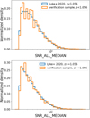 |
Fig. 1 Distribution of the median S/N for low-redshift (top) and high-redshift (bottom) of the verification sample (orange), compared with the parent sample (blue). |
Initial kinematics and bounds of model components.
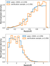 |
Fig. 2 Redshift distribution for low-redshift (top) and high-redshift (bottom) sources of the verification sample (orange), compared with the parent sample (blue). |
2.2 Model construction
We implemented a function that constructs a model following the pPXF structure and recipe, meaning that this function returns all the arrays that are needed or are optional input for the pPXF fitting, with the exception of the spectrum, noise, and mask that are generated in the data preparation step. There are two sets of four models (eight in total) that can be constructed (see Sect. 3 for details on the actual implementation). We describe these models below:
Model-1: this model is composed by templates for stellar populations from the E-MILES library (Vazdekis et al. 2016), a set of power laws for the AGN continuum (AGN-cont), a set of Gaussians for narrow emission lines (NELs), a set of Gaussian profiles for Broad emission lines (BELs), Balmer higher-order emission lines (H8-H50) together with the Balmer continuum (BHO-cont) templates, and FeII UV/optical pseudo-continua templates (Boroson & Green 1992; Vestergaard & Wilkes 2001). The AGN-cont model is fitted as
 , with λ being the wavelength, N the wavelength normalization factor, and α the slope of the power law. For all the models, we used N = 5000 and −3 ≤ α ≤ 0 in steps of 0.1.
Model-2: this model adds to the model-1 a second set of BELs.
Model-3: this model adds to model-1 a pair of Gaussian profiles to represent emission lines from winds in the [OIII]5007 doublet region. This component is called [OIII]winds.
Model-4: this model adds the second set of BELs and the [OIII]winds to model-1 (i.e., model-4 combines the additions of model-2 and model-3).
In all cases, all the lines grouped in one set of NELs or BELs have all their kinematic moments linked. With the exception of the broad CIV emission line, which has individual kinematic moments. Each individual line, as well as each (pseudo-)continuum template, is scaled by free and independent normalizations, except for line doublets with fixed relative normalizations. In general, each set of templates is a component of the model and each template in a component has the same kinematic moments and independent normalizations.
The second set of models is identical to the ones mentioned above, with the difference that there are no stellar population templates. These models are used for objects with redshift z > 1. This value is conservative, based on the stellar population intensity observed in quasars, where for objects with z > 0.8 the host galaxy contribution becomes negligible (Vanden Berk et al. 2001; Jalan et al. 2023). Henceforth, we refer to both models with and without stellar population templates as model-1, model-2, model-3, or model-4, and only discriminate them when necessary.
We followed the pPXF recipe to input the initial kinematic values and to restrict them for the components in each model. These values are summarized in the Table 1. The selection of these values was guided by the typical values of the different components observed in AGNs and by the test of restrictions to obtain a good fit after visual inspection in previous works by the authors (e.g., López-Navas et al. 2022, 2023; Bernal et al. 2025). In particular, for the bounds values of the velocity shift of CIV we consider the measured values observed in different works about CIV (Coatman et al. 2016, 2019; Gillette & Hamann 2024). pPXF offers the option to fit the skewness and kurtosis for any kinematic component. We used these parameters for stellar templates and BELs, including CIV. In the workflow, we fit the spectra in rest-frame wavelengths, which means that the initial value for the first kinematic moment in pPXF, the velocity shift, is always zero for model-1. However, the initial velocity for the two BEL components in model-2 and model-4 and, for the [OIII]winds component in model-3 and model-4, it is nonzero. In the case of the BEL components, the fitted velocity with model-1 was used as the input initial velocity, while for the [OIII]winds, a blue shift initial velocity is used. In addition, the initial velocity for the NEL component, after the first fit with model-1, can be nonzero if this is determined by the routine that produces the recommendation (see Sect. 3). In pPXF, the best fit is determined by minimizing the chi-squared between the data (spectrum) and the pPXF-model. The pPXF-model is the input model convolved with the kinematic moments (velocity shift, velocity dispersion, skewness, and kurtosis) determined by pPXF routine. We note that in the pPXF scheme, each component has its own kinematic moments (velocity shift and velocity dispersion) and all the templates in each component share the same kinematic moments. As mentioned, all the values used are typical for AGN spectra but are easy to modify when required.
3 Discrete wavelet transform of the fit residuals: Best model recommendation
Here, we present the implemented routine used to detect structure in the fit residuals and to recommend, when appropriate, a new model for spectral fitting.
3.1 Regions of interest
In the first part of the routine, regions of interest were generated. We selected regions containing BELs that are used to estimate single epoch black hole mass (Mejía-Restrepo et al. 2016), namely, Hα, Hβ, MgII, and CIV. In addition, the region [OIII]λλ4960, 5008, and the [OIII] windsλλ4960,5008 were also considered as regions of interest. Both regions [OIII] and [OIII] winds refer to the doublet emission lines 4960 Å and 5008 Å. The wavelength ranges for these regions were determined using the central wavelength of each emission line, with the limits set to three times the typical velocity dispersion of that line on either side. For these, we considered the central wavelength of each emission line for BELs and the centers 4960 Å and 5008 Å in the case of the [OIII] and [OIII] winds, with widths of ±6000 km/s for BELs and ±900km/s for [OIII] and [OIII] winds. Then, to determine which regions are included in the following analysis, we implemented a limit where the regions of interest must be at least 50 Å from the edges of the spectrum. These limits help to avoid truncated regions in the analysis, when they are at the extremes of the spectrum.
3.2 Discrete wavelet transform
Next, the routine uses the wavedec1 function from the package pywt (Lee et al. 2019). This function performs 1D multilevel discrete wavelet transform (DWT) decomposition of the given signal and returns an ordered list of coefficients which capture the details and overall trend of the signal. The wavedec function requires as input the signal, wavelet function, mode, and decomposition levels. The signal in our case is the best-fit residuals. For the wavelet function, we used the Haar functions, which offer a fast decomposition, and easy interpretation for the purposes of this work. Other functions such as Daubechies and Symlets can also be used, but they will require a change in the interpretation algorithm. Then, for the residuals represented as the signal r = {r1,..., rk}, the representation at level j is
![Mathematical equation: r\xrightarrow[]{DWT}\{ a_j[k],d_j[k]\},](/articles/aa/full_html/2026/03/aa56748-25/aa56748-25-eq2.png)
where aj [k] and dj [k] are the approximated and detailed coefficients, which are calculated using the Haar filters as
![Mathematical equation: a_j[k]= a_{j-1}[2k] \frac{1}{\sqrt2}+a_{j-1}[2k-1] \frac{1}{\sqrt2} ,](/articles/aa/full_html/2026/03/aa56748-25/aa56748-25-eq3.png) (1)
(1)
![Mathematical equation: d_j[k]= a_{j-1}[2k] \frac{1}{\sqrt2}-a_{j-1}[2k-1] \frac{1}{\sqrt2} .](/articles/aa/full_html/2026/03/aa56748-25/aa56748-25-eq4.png) (2)
(2)
In this definition, the aj [k] and dj [k] coefficients for j = 0 are the r = {r1,..., rk} signal values (in our case, the residuals), k the index of the coefficients at each level j, and the use of indexes 2k and 2k - 1 denote the downsize by two from one level to the next (i.e., each level will have half as many coefficients as the previous one).
For the mode, we used the smooth option that refers to smooth-padding and where the signal is extended symmetrically on the edges (rsmooth = {r2, r1, r2,..., rk-1, rk, rk - 1}) and for the levels, we used four (see details in the next section). With these parameters, the wavedec function generates in total five arrays, four for the detailed coefficients at levels [1,2, 3,4] and one for the approximated coefficients at level [4]. The use of the DWT with other applications can be found in Stollnitz et al. (1995).
3.3 Detection of structure in the residuals
Using the downsizing by two, the signal width enclosed by the coefficients at each level can be calculated. For this, we used the velocity-scale, which is the difference in km/s between two pixels. This value is constant for a logarithmic binned spectrum such as SDSS data. For the SDSS spectra, the velocity-scale is 69.15 km/s. Therefore, for the second decomposition level, four pixels are enclosed by each coefficient, equivalent to 277 km/s. This wavelet size in km/s lies in the NEL velocity dispersion range. Therefore, we can use the detailed coefficients of the first and second decomposition levels to detect narrow structure in the residuals, in particular to detect the presence of winds in the [OIII] region. For the third decomposition level, eight pixels are enclosed by each coefficient, equivalent to 553 km/s, while they are twice as broad for the fourth level. Therefore, for the third and fourth decomposition levels, the coefficients can be associated with residual structure in the broad line regions.
To detect and flag structures in the residuals, we computed the square of the coefficients at each level and identified deviations as values that exceed a predefined threshold. This threshold is calculated for each level as
 (3)
(3)
where σsc is the standard deviation of the square of the coefficients, len(sc) is the number of coefficients, and fc is a factor to apply a more or less stringent threshold. This relation with fc = 1 was probed to be optimal to find significant deviations in the statistical study of Donoho & Johnstone (1994). However, for our study, we compared results with different threshold values of fc = [0.75,1.00,1.25,1.50,1.75,2.00,2.25,2.50].
Next, the routine checks if the flagged deviations are in the regions of interest. For this purpose, the wavelength index of the deviations in the coefficients is related via the expression,
 (4)
(4)
where dvi is the index of the i - th deviation, len(sc) is again the number of coefficients, and len(residuals) is the number of pixels in the residuals. This allows us to determine the wavelengths at which the deviations are detected at each level, as well as well as to identify the regions of interest where these deviations occur.
3.4 Model recommendation
The flagged deviations in the regions of interest and conditions in the other input parameters are then used to determine the model recommendation. The model recommendation options are named: Two-BELs, [OIII] winds, and Two-BELs + [OIII] winds. The routine recommends the Two-BELs, that is equivalent to model-2, if one of the following conditions is fulfilled:
Gaussian deviation and residual structure. Here, the absolute value of one of the skewness or kurtosis moments of the BELs component is greater than 0.05, and the other is greater than 0.04, and at least one residual deviation in levels [3,4] is detected in at least two of the broad line regions Hα, Hβ, MgII, and CIV. Skewness and kurtosis values of 0.04 and 0.05 correspond to visually significant deviations from the Gaussian profile that cannot be attributed to noise.
Residuals structure in more than one region. For this case, the number of deviations in levels [3,4] is greater than four and deviations are detected in at least two broad line regions.
-
Only one BEL region in the spectrum or only one with relatively large residuals. Here, at least one deviation in levels [3,4] is detected in only one broad line region and the significance of the absolute residuals is higher than 10 (Eq. (5)). This value for the significance was set based on empirical testing with a large set of spectra with high residuals. In particular, objects where the observed wavelength range only includes one BEL region for the analysis. For the significance of the absolute residuals in a given region, we used the equation
 (5)
(5)where I(|r|) is the integral of the absolute residual values in the given wavelength range, and unc(I(r)) is the uncertainty in the integrated residual flux, approximated as
 (6)
(6)with σR being the standard deviation of the residuals, N the number of pixels, and ∆λ the wavelength step, all in the region of interest.
For the [OIII] winds recommendation, which is equivalent to model-3, the routine considers only the region [OIII] winds and the levels [3,4] of the DWT decomposition. These levels allow for the detection of deviations on scales larger than 500km∕s. The recommendation is set if the following conditions are accomplished:
-
The region of [OIII] winds is not well fitted. Here, we require at least one deviation and residuals significance >2.5 from the [OIII] winds region. Once more, this value for the significance was set based on empirical testing with a large set of spectra with high [OIII] winds residuals. The significance of the residuals is calculated in a similar way as before
 (7)
(7)for the [OIII] winds region of interest. We note that here we use the integral of the residuals and not the absolute residuals, as done in Eq. (5)).
There is structure detected in the residuals, with at least one deviation, and the NELs are fitted with a relatively large velocity dispersion, greater than 300 km∕s.
The Two-BELs + [OIII] winds model recommendation is the result of having both Two-BELs and [OIII] winds recommendations and it is equivalent to model-4.
If none of the conditions described for the Two-BELs or [OIII] winds recommendations are met, the result is the No-new-model recommendation. This indicates that the routine found insufficient evidence to justify a more complex model as a better option for fitting the spectrum. When the result is No-new-model, the routine computes the residual significance of each region, following Eq. (7). When this significance is greater than 2.5, the routine produces a comment with the region name and the significance value as a warning that can be used for a later visual inspection of the best-fit.
The final result from the routine is the model recommendation and the comment about broad line regions. Additionally, during the routine, two tables are saved: one with the region name, DWT level, and number of deviations, and another table with the region name and residuals significance using Eq. (7).
4 Best model selection
When the result from the DWT routine is a new model recommendation, a second fit is performed using the recommended model. To establish if the second fit really produces a better fit and the recommendation is not a false-positive, we implemented a score based on the normalized root-mean-square (RMS) difference and F-test, which takes into account detailed mismatches in the regions of interest (i.e., around the emission lines) as well as the overall fit across all wavelengths.
The RMS difference is computed as

where RMS 1 is the RMS of the first model best-fit and RMS 2 is the RMS of the second model best-fit. Based on the RMSdif values, the qualitative results and assigned scores are:
Significant improvement with score = 1, if RMSdif > 0.1.
Partial improvement with score = 0.5, if 0.01 < RMSdif < 0.1.
No significant improvement with score = 0, if −0.01 < RMSdif < 0.01.
Slight worsening with score = −1, if −0.1 < RMSdif < -0.01.
Significant worsening with score = −100, if RMSdif < -0.1
The RMS scoring is performed both for the global wavelength range and each of the following regions of interest: Hα, Hβ, MgII, CIV, and [OIII], when they lie within the spectral range. in addition, for the global wavelength range, an F-test is performed between the first and second best-fits. A p-value < 0.05 is used to determine if the improvement is significant, and results in an assigned score of score = 2. On the other hand, when the p-value > 0.05 the assigned score is score = −1. This score for the F-test is assigned to corroborate that the total fit significantly improves.
To determine which of the fits is better, we added the global RMS, local RMS, and F-test scores. If the total score is equal to or greater than one, the second model is selected as the best fit, and we save all the results from the pPXF fit for any further calculation and analysis. In the other case, if the total score is smaller than one, the first best-fit result is saved for subsequent analysis. We opted for this local and global score system because of the degeneracy between templates, given that for some cases the use of a model with more templates for a region of the spectrum can result in the local improvement but worsen the continuum.
In Fig. 3, we show an example of the best-fit with model-1 (three top panels) and the best model, after the recommendation and algorithm decision, which was obtained with model-3 (three bottom panels). This means that the algorithm analyzes the residuals and other parameters to determine that model-3 can produce a better fit, and after comparing both fits, the best model selection resulted in model-3. The plot shows a zoom into regions of Hβ and MgII emission. In the Hβ region, it is apparent that model-1 misses the [OIII]winds, which are well fitted with model-3. Note that this is an example of the automatic result of the algorithm. More examples are presented in Appendix A.
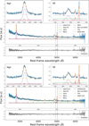 |
Fig. 3 Comparison of the best-fit of a spectrum fitted with model-1 (three top panels), and model-3 (three bottom panels), the last was the final result from the code. The Hβ and MgII regions are zoomed, and the total fit and residuals are also shown. The main difference between the two fits is the use of [OIII]winds. Dashed lines delimit the region where the DWT flagged the residuals structure (see Appendix A). All panels have the same arbitrary units on y-axis. |
5 Algorithm validation
To ensure that the best model determined by the algorithm is statistically consistent with the decision that can be made by human visual inspection, a group of eight people with different expertise in AGN spectral fitting collaborated with the validation process. These individuals are referred to as validators. In the method used for the validation, each of the 800 objects was inspected by three validators. All the objects were randomly distributed among them so that any group of three validators shared only a fraction of the total number of objects that each validator inspected and all validators inspected 300 objects.
For the visual inspection, validators had access to the plot of the best-fit of the spectrum using model-1. In the plot, the top panels show a zoom in the regions of interest, which are determined by the redshift of the object. The middle panel shows the total wavelength range fit with the different components, and the bottom panel shows the residual of the best-fit. The top three panels in Fig. 3 are an example of these plots.
After inspection, the validators decided whether to add or not more components to improve the fit. They were provided with the same options given to the algorithm: No-new-model, Two-BELs, [OIII] winds, and Two-BELs + [OIII] winds. Validators could also add a comment for each object to note features such as complex BELs or noisy spectra, among others.
6 Results
6.1 Algorithm time performance
This work aims to automate the recommendation of additional model components and the selection of the best model for fitting a large sample of AGN spectra, thereby eliminating the need for visual inspection and reducing the time required for spectral fitting. Here, we report and compare the computational time for the validation sample in different steps of the algorithm. We define the following steps of the algorithm: The first fitting using pPXF, the determination of a recommendation by the DWT routine, and the second pPXF fit. To do a fair comparison for the computational time spent in the first pPXF fitting, we divide the objects by their redshift, because for objects with z < 1 the inclusion of 350 stellar population templates has an impact on this time. We did not make the same separation for the second pPXF fitting because we only used the stellar templates that result in the first best-fit model; in most cases, this is less than four, leading to a negligible impact on the fitting time.
Table 2 shows the 10th, 50th, and 90th percentiles of the time taken by the aforementioned steps, as well as the total algorithm time. Since there is a small difference (2s for z < 1, and 1s for z > = 1) for the 50th percentile of the total time when considering the different thresholds (different factor fc) used for the identification of deviations, we report the longest time among all the time distributions (obtained when fc = 0.75). These results show that for 50 percent of the objects with z < 1 the algorithm ends in less than 29s, and for 90 percent in less than 75 s. While for objects with z ≥ 1, in less than 7s for the 50 percent and in less than 18 s for the 90 percent. For comparison, validators were asked to report the time spent during the visual inspection. From these data, we found that a person with expertise in modeling this type of spectra spends an average time of 60 seconds on visual inspection, which implies the inspection of the fit by zooming into the different regions of interest, the decision of the new model, and manually setting the new model. Meanwhile, the model recommendation step for the routine is completed in less than 1 s for 50 and even 90 percent of the objects (and is also the case for the 98 percent in all the fc cases).
The time values were produced with the use of a personal computer, MacBook Air (M1, 2020)2. We conclude that the time saved by applying the algorithm, of about 60s per spectrum, is significant compared to the total fitting time of 75 s or less, even in a middle-range personal computer. This time saving can be more significant when using more computational power and parallel code execution.
Algorithm computational time.
6.2 Validation results
Another objective of this work is to automatically determine the model that fits the spectrum best. Here we show the comparison of the decision in the best-fit model between validators and between the validators and the algorithm.
6.2.1 Validators comparison
When comparing the decision between two validators, we define coincidence in recommendation if the recommended model is the same or if one of the validators recommends model-4, while the other recommends model-2 or model-3, meaning that both validators coincide in at least one of the possible modifications for the model to be used in the second fitting. In Table 3, we present the pair of validators, the number of objects in common between both validators, and the fraction of coincidence. The minimum coincidence between validators is 0.72, the median is 0.90, and the maximum coincidence is 1.0. In Table 3, we also show the number of objects and the coincidence fraction between validators for the cases with redshift z < 1.056 (i.e., with 4 model options) and z > = 1.056 (i.e., with 2 model options).
We compare the rate of coincidences with the results of a random choice by re-shuffling the model choices made by each validator and re-calculating the fraction of coincidence. For this test, the validator pairs and the objects they had in common were kept fixed, but the model choices assigned to each object were shuffled randomly, within the choices made by each validator. In this way, the experiment retains the overall probability that a given validator will choose a given model. The median rate of coincidence between these random choices was 0.79 ± 0.01 for objects with z < 1.056 and 0.80 ± 0.01 for objects with z >= 1.056.
For the two cases, z < 1.056 and z > 1.056, the median coincidence between two validators is larger than the random probabilities. We notice here that for z < 1.056 the median fraction of objects where the validators recommend a new model is 0.19 and for z > 1.056 it is 0.02. Showing that only a relatively small number of objects in the sample required a more complex model to be fitted, according to the validators. We discuss this in Sect. 7.
Coincidence between two validators.
6.2.2 Algorithm and validators comparison
Here, we compare the recommendation made by the validators and the best model determined by the algorithm. In a similar way as between two validators, coincidence is defined as when the algorithm and validator agree on the model, or when one of them chooses model-4, while the other chooses model-2 or model-3.
In Fig. 4, we show the median value and standard deviation of the coincidence fraction between the algorithm and validators. We compare the results with the random median fraction of coincidence obtained by re-shuffling the model choice by each validator. This random median fraction of coincidence keeps the number of choices of each model by each validator, and then compares them with the real model selection. Results show that the coincidence fraction is systematically and significantly higher than the random coincidence. The coincidence fraction for objects with z < 1.056 has values between 0.76 and 0.80, with standard deviations between 0.06 and 0.09. While for objects with z > 1.056, the coincidence fraction has values between 0.91 and 0.96, and standard deviations between 0.05 and 0.06. In Appendix B we present the tables with all the comparisons between the algorithm and the validators for each fc value, and for the cases of comparing all the objects and when comparing objects separated by z = 1.056.
We compare cases where the best model of the algorithm is model-1, and the validator recommendation is a different model, meaning that visual inspection suggests the addition of a [OIII] winds and/or a BEL component; we call this case a complexitydiscrepancy. We also compare the opposite case, where the validator recommendation is model-1 while the algorithm’s best model is any different option; we call this case simplicitydiscrepancy. All the results for the complexity-discrepancy and simplicity-discrepancy are in Appendix B. The median values for complexity-discrepancy range between 0.09 and 0.10 for z < 1.056, and are always 0.02 for z > 1.056. For the simplicity-discrepancy, the median values are between 0.09 and 0.14 for z < 1.056, and between 0.02 and 0.08 for z > 1.056. For completeness, the tables in Appendix B also present the fraction of other discrepancy cases, different to complexity- or simplicity-discrepancy, and meaning that when the algorithm or the validator recommends [OIII] winds, the other recommends BEL (only possible for z < 1.056). This fraction is 0.01 for z < 1.056 only in a few cases.
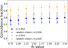 |
Fig. 4 Coincidence ratio between the algorithm and each validator. The mean coincidence across all validators is shown in markers, and the root-mean-squared scatter of coincidence ratios is represented by the error bars. Blue marks are for objects with z < 1.056 and orange marks for z > 1.056. The small markers (same color code) represent the random median fraction of coincidence obtained by the re-shuffling of the model choice by each validator. |
6.3 Comparison with synthetic data
The main goal of the algorithm using the DWT method is to identify when a better fit of a spectrum can be obtained by the use of a more complex model. Here, we present the results obtained using synthetic data and compare them with those from our code.
6.3.1 Synthetic spectra generation
We generated synthetic spectra in the same observed wavelength range as SDSS spectra for redshifts of 0.5, and 1.8. We used the pPXF-util functions to generate the emission lines (NELs and BELs). To obtain a fixed value for the FWHM we convolve them using the gaussian_filter1d, and for all the synthetic components, we used the log_rebin function to obtain the same binning as an SDSS spectrum. The fixed FWHM for BELs was 5000km∕s for z = 0.5, 7000km∕s for z = 1.8. For NELs we adopt FWHM= 400 km/s. For the relative intensity of NELs and BELs we used the relative fluxes reported in Vanden Berk et al. (2001). For the synthetic AGN-continuum we used the power-law function  . We used three stellar populations templates from the E-MILES library of 0.5Myr, 5Myr, and 11Myr with relative intensities between them of 0.5, 0.3, 0.02 to generate a synthetic stellar population component (only for z = 0.5). In addition, we added a UV/optical FeII component. We fixed the AGN-continuum luminosity at 5100À or at 3000 Å, depending on redshift, to be Lλ = 1045 ergs/s. Then, for the relative intensity of the other components with respect to the synthetic AGN-continuum, we adopt empirical relations. For the relative flux of BELs, we used the relations
 (8)
(8)
 (9)
(9)
The Eq. (8) is from Greene & Ho (2005), and Eq. (9) from Shen et al. (2011). With this relation, we obtain a factor to multiply our BELs templates. For NELs we impose a factor to obtain the Hß narrow flux to be 12% of the broad flux for z = 0.5; whereas for z = 1.8, NELs have a contribution of 0.3% of the emission lines. For the stellar component, we imposed that it contributes to 10% of the total continuum for z = 0.5. For FeII, we used the relation RFeII = 0.5 × (FWHMHβ/4000.0)−1.0, where RFeII = FFeII,λ4750/FHβ (Boroson & Green 1992).
Additionally, for z = 0.5 we generate three templates of [OIII] winds. These outflows have 100%, 50%, and 20% of the [OIII] flux and were blueshifted 346km/s (Zhang et al. 2011). In addition, we generated a second set of BELs with FWH= 10000 km/s and imposed 30% the flux of the first BELs to obtain spectra with more complex broad regions. For z = 1.8, the CIV emission line is in the wavelength range and, in this case, we shifted the emission by adding an outflow emission with FWHM= 10 000 km/s and blueshift of 1000 km/s. Before adding the different components, all were convolved to the SDSS instrumental FWHM using the function fftconvolve3 Finally, we add noise to the spectra using the inverse variance of SDSS spectra with magnitude in g-band ~ 18 mag (which is the approximate g-mag for an object of L5100 = 1045 ergs/s and z = 0.5). For noise, we use spectra with SN_MEDIAN_ALL=[5,10,20,30]). We obtained a synthetic inverse variance per pixel and then used these values to generate random noise using a normal distribution centered at zero. With this method, the synthetic SN_MEDIAN_ALL results in similar values as the SDSS spectra.
We generated 45 spectra in total. For z = 0.5 we have: one with the initial description (NELs+BELs+AGN-cont+FeII+sterllar-cont; similar to model-1), three with the addition of [OIII] winds (similar to model-3), one with the addition of second BELs (similar to model-2), and three with the addition of a second BELs and [OIII] winds (similar to model-4). For z = 1.8, we obtained one spectrum with the initial description without a stellar component (similar to model-1). And for each of the mentioned nine spectra, we obtained a spectrum with the different SN_MEDIAN_ALL values.
Coincidence fraction by SN_MEDIAN_ALL and fc.
6.3.2 Results for the synthetic spectra
We adopted the same methodology using fc values of [0.75,1.0,1.25,1.50,1.75,2.0,2.25,2.50] and compared the synthetic model with the best model proposed by the code, and the synthetic flux of the different emission lines with the flux of the best model fit.
In Table 4, we compare the coincidence fraction between the code and the synthetic spectra with the different SN_MEDIAN_ALL values. The coincidence fraction (with the same meaning as in the validation results) is compared for the best model selected by the code with different fc values. Tables with the comparisons for each synthetic spectrum are in Appendix C. From Table 4, we can say that, on average, using fc = 0.75 obtained better coincidence, and that fc = 2.5 obtained the lower values of coincidence. However, when we consider spectra with SN_MEDIAN_ALL≥ 10, values between fc = 0.075 and fc = 1.75 give the same coincidence fraction, and fc = 2.0 produces similar or higher values. We notice that spectra with SN_MEDIAN_ALL= 5 show a profile where noise buries the second BELs and/or [OIII] winds for the visual inspection.
We compared the flux of the synthetic spectra emission lines with those obtained from the best model. In Figs. 5 and 6, we compare the narrow and broad emission lines flux for spectra with z = 0.5, which have all the synthetic spectrum cases. In these figures, the y-axis is the fractional difference between the modeled-flux fm and the synthetic-flux fs ([fm - fs]/fs). For the NELs Hα, Hβ, [OIII], and [OIII]wind are in Fig. 5, and for the BELs Hα, Hβ, and MgII in Fig. 6.
In Fig. 5, we observe that Hα and [OIII] are in good agreement with the synthetic flux for spectra with SN_MEDIAN_ALL> 5, while Hβ and the [OIII]winds are in good agreement only for a few cases. In the case of Hβ, the scatter is a result of the embedded narrow emission in the broad component. While for [OIII]winds, we found that for the synthetic blue-shift, the wind component is well fitted if the wind flux is comparable with the narrow emission flux; in the other cases, the noise and narrow component can hide the outflow. For BELs, Fig. 6 shows that when the emission line is more intense, the flux agreement is better, and also that a poor S/N in the emission line region can lead to a large scatter in the measurements of the flux. We note that this flux comparison is not a test of the quality of pPXF fitting and only aims to test the code fitting results for completeness.
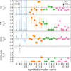 |
Fig. 5 Fractional difference between the modeled flux, fm, and the synthetic flux, fs, for NELs. Colors indicate the SN_MEDIAN_AL of the synthetic spectrum, and marks indicate the S/N in the region of the emission line labeled on the y-axis. In the x-axis of the bottom panel the names of the synthetic models are presented: w00, w02, w05, and w10 are the reference for the percentage of [OIII]winds which are 0%, 20%, 50%, 100% of the [OIII] NELs. The “2bels” label is a reference to synthetic models with two BEls components. |
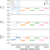 |
Fig. 6 Fractional difference between the modeled-flux fm and the synthetic-flux fs for BELs. Colors indicate the SN_MEDIAN_AL of the synthetic spectrum, and marks indicate the S/N in the region of the emission line labeled on the y-axis. In the x-axis of the bottom panel, the labels are the same as in Fig. 5. |
7 Discussion
Performing the task of analyzing thousands of spectra is becoming a more commonplace scenario. Surveys such as SDSS-V, DESI, and the future 4MOST are targeting large samples of AGNs and AGN candidates, and making the data public. Therefore, we need computational options to reduce the time used to produce measurements of population properties, which can increase the efficiency of the scientific analysis. Here, we present an algorithm that can improve the efficiency of the AGN spectral analysis by automatically selecting the best model to fit the spectra. In the following, we discuss the advantages, limitations, and options to mitigate them, as well as our outlook for future works.
7.1 Advantages
The automated method implemented for the best-model selection depends on the value of a few parameters, which means that the results can always be replicated. Meanwhile, the choice of the best-model by visual inspection depends on the expertise and level of fatigue of the human in charge of the task, as shown by the validators comparison in Sect. 6.2.1. This reproducibility advantage helps to reduce the subjectivity of these decisions and final results.
One of the great advantages is the computational time of the algorithm as an automatic method compared with the estimated time that a human validator should invest. From the validation process, we estimate that the time spent in the visual inspection for one object is 60s, while for the same task, the algorithm uses less than 1 s. Considering the 60s as average time, we can estimate that for a sample of 10 000 objects, and the mean recommendation percentage of a new model of 23%, a human will need a total of 38.3 hours of work only for the visual inspection of the spectra with new model recommendation. In comparison, a computer with similar characteristics to the one used in this work will perform the automated inspection of all the objects in 2.8 hours. This is an important difference if we take into account that a human is not capable of carrying out the total visual inspection continuously and would require more than two working days to cover the 38.3 hours. We note that this time scales with the size of the sample. Moreover, we compared the results of the algorithm with the visual inspection. The comparison shows that if we consider the comparison between two validators (Sect. 6.2.1), and between the algorithm and one validator (Sect. 6.2.2), the algorithm reach a similar coincidence fraction with validators (between 0.76 and 0.80 for z < 1.056, and between 0.91 and 0.96 for z > 1.056) as the coincidence between two validators (0.82 for case z < 1.056 and 0.98 for z > 1.056).
As mentioned in the Sect. 1, the algorithm is implemented in Python, which is currently one of the most popular code languages and can be executed in all (albeit not highly specialized) operating systems. This characteristic makes it easy for users to implement the algorithm code and to modify the needed values for other cases, such as the detection of asymmetry in BELs or absorption features near BEL regions. Adding new regions of interest of the spectrum to inspect additional emission lines or continuum profiles can also be easily implemented. Finally, the algorithm can be implemented for any instrument spectral data with small modifications or additions. This flexibility for improvement is a great advantage of the algorithm.
Another feature indicated in Sect. 3 is the output of comments for specific regions considering the residual significance. As a function of the different fc values, the fraction of objects with comment outputs are [0.11,0.09,0.07,0.06,0.05,0.04,0.04,0.03], respectively. In this work, we do not present more analysis of the comments output because those are specific to each object, and the analysis of these particular cases is beyond the scope of this paper. However, we note that these features can be used to find and study particular cases in large samples, such as to identify anomalous objects.
7.2 Limitations
As the objective of automatically fitting thousands of spectra is to extract properties of these objects, we examine here some caveats in the algorithm that lead to the fraction of disagreement among validators, and for this small fraction, a probable inaccurate measurement of these properties.
The disagreement between the best model from the algorithm and the recommendation of the validators can be affected by spectral quality. The significance of residuals, which is used to determine the model recommendation, is directly affected by the quality of the data in each region of interest. In cases of good quality, small structure in the residuals can be identified, while in low-quality spectra, the structure can be diluted by the larger scatter among the residuals, as shown in Sect. 6.3.2. It is more frequent that this large scatter occurs when the regions of interest lie near the edges of the spectra, where the data can suffer from larger noise.
Additionally, as mentioned before, anomalous spectra might be included in large samples and the quality of the fit in these cases could be limited by the models included. As we used pPXF, by the initial values and bounds of the kinematic parameters as well. For example, double-peaked BELs (i.e., double broad emission lines with a large difference in velocity shift) will require different initial values for the first kinematic moment. Even when the model with double BELs is recommended, the bounds of the kinematic values can prevent a good fit, since the double BEL scenario in the algorithm is set up to model lines with different velocity dispersions, but not a large difference in velocity shift. We alleviated this shortage for C IV emission lines, which can show blushifted outflows (Gaskell 1982; Wilkes 1984; Tytler & Fan 1992; Temple et al. 2023) by modeling this emission as an individual component, meaning individual kinematic values. Another example is the broad absorption line (BAL) objects (Liu et al. 2015), where the implemented models are not able to fit spectra due to their strong absorption profiles. Furthermore, even when the algorithm recommendation suggests an extra component, the fit does not improve because of the model limitations.
Another factor that limits the performance of the algorithm and the final fit is the presence of unflagged bad-pixels in the emission lines being modeled, which produce false deviations during the DWT decomposition and/or the incorrect measurement of quantities such as the flux or equivalent width of emission lines. Also, high inaccurate redshift values associated with the spectra will lead to an incorrect fit and false flux deviation measurements. Small inaccuracies can be compensated by the freedom to fit a velocity shift to all the components, but this is limited to velocities of ±500km/s (being higher for CIV) in the current setting.
7.3 Potential for optimization
The presented algorithm has important characteristics that can be expanded to a higher level of complexity. One of these is the possible addition of more fitting models or variants of the ones presented here. New conditions can be added to discriminate particular cases and use more appropriate models. Another possibility is the use of the signs of the DWT coefficients to find strong absorption features, as in the case of BALs objects. As mentioned before, the model recommendation and the best-fit decision depend on a few parameters, such that a more exhaustive test of the algorithm using a grid of values for the different parameters could lead to an increase in the efficiency of the algorithm. A more sophisticated approach could be to use a dynamic threshold value for deviation detections in the DWT decomposition, where the threshold could be optimized for each object and each region, associating the threshold with the quality of the data. In our test, we found that fc values from 1.25 to 2.50 have similar coincidence and discrepancy results. Based on these results, a moderate threshold of fc = 1.75) is recommended. This value allows for a more complex model in the second fit when needed, while the best-model selection routine (as the final decision step) can prevent the use of unnecessarily complex models. Another potential application is to use the deviation detection when comparing different epochs of the same object, to facilitate the detection of changing-look-AGNs, changing-state-AGNs, and even newborn or quiescent AGNs in large data samples.
In the bigger picture, the code where the algorithm is implemented can be modified to use different types of data archives from different instruments. For example, it would be easy to apply the algorithm to DESI and future 4MOST data, for instance. Moreover, the algorithm has no strict dependency on pPXF output and could be implemented in a routine with different software. Finally, the method is not restricted to the UV/optical wavelength range and can be used in other wavelength regimes (e.g., XSHOOTER, MOONS, PFS, SPHEREx).
8 Summary
We present an algorithm implemented in Python to perform automatic best-fit model decisions for AGN spectra. The algorithm uses the pPXF software for spectral fitting, the DWT method for model recommendation, and RMS and F-test assessment to obtain the best model decision.
We implemented two sets of four different models, which can be used for the spectral fitting. The difference between models is in the use of extra Gaussian components for BELs or [OIII]winds. The workflow uses the simplest model for the first fit, and a dedicated routine recommends whether or not to use more complex models. This routine is based on the detection of deviations in the DWT decomposition of the best-fit spectrum residuals, residual significance, and kinematic parameters from the first best-fit. The detection of deviations depends on a threshold value. We tested different threshold values and implemented the DWT routine in the specific regions Hα, Hβ, MgII, CIV, and [OIII], but more regions can be added if needed.
To validate the method, we used a sample of 800 spectra from Lyke et al. (2020) catalog, which is a sample of SDSS quasars, spanning a wide range of redshifts. The first fit of these objects was visually inspected by eight validators, with each spectrum inspected by three different validators. For comparison, the validators had the same options as the routine for the model recommendation. We compared the coincidence in recommendations between validators and between the algorithm and the validators. When comparing two validators, the median fraction of coincidence is 0.82 for z < 1.056 and 0.98 for z > 1.056. The comparison of the algorithm, using the different values of fc, and each one of the validators results in a median coincidence between 0.76 and 0.80 for objects with z < 1.056 and between 0.91 and 0.96 for z > 1.056.
We also compared the computational time with the time spent on the visual inspection. For the visual inspection task, the algorithm in 90% of the spectra uses less than 1s. In contrast, we estimate that a validator spent 60s in the visual inspection. Furthermore, for 50%(90%) of the spectra where a larger number of templates were used for the fit, the algorithm is completed in less than 29s(75s). In conclusion, the use of the presented algorithm is more efficient than the visual inspection when larger samples are fitted. Considering the results, we found that the most adequate and equilibrated threshold resides between fc = 1.25 and fc = 1.75, but a more stringent (higher) fc value can be better in particular cases or for specific studies.
Finally, we highlight the accuracy of the algorithm measured by the coincidence fraction and the computational time advantage. The limitations are more restricted to the quality of the spectra, particular cases, and the subjectivity in the visual inspection. Additionally, we propose further development of the code to improve the results and expand its use for particular studies.
Data availability
The algorithm scripts are publicly available on this GitHub repository: https://github.com/santiagobg/amaru_v01 and at the CDS via https://cdsarc.cds.unistra.fr/viz-bin/cat/J/A+A/707/A206
Acknowledgements
The authors acknowledge the National Agency for Research and Development (ANID) grants: Programa de Becas/Doctorado Nacional 21212344 (SB); Millennium Science Initiative Programs NCN2023_002 (SB, PA, PL, MLM-A); BASAL CATA FB210003 (FEB), FONDECYT Regular 1241005 (FEB, PA), Millennium Science Initiative, AIM23-0001 (FEB), and the China-Chile Joint Research Fund CCJRF2310 (MLM-A). Funding for the Sloan Digital Sky Survey IV has been provided by the Alfred P. Sloan Foundation, the U.S. Department of Energy Office of Science, and the Participating Institutions. SDSS-IV acknowledges support and resources from the Center for High Performance Computing at the University of Utah. The SDSS website is www.sdss4.org. SDSS-IV is managed by the Astrophysical Research Consortium for the Participating Institutions of the SDSS Collaboration including the Brazilian Participation Group, the Carnegie Institution for Science, Carnegie Mellon University, Center for Astrophysics | Harvard & Smithsonian, the Chilean Participation Group, the French Participation Group, Instituto de Astrofísica de Canarias, The Johns Hopkins University, Kavli Institute for the Physics and Mathematics of the Universe (IPMU) / University of Tokyo, the Korean Participation Group, Lawrence Berkeley National Laboratory, Leibniz Institut für Astrophysik Potsdam (AIP), Max-Planck-Institut für Astronomie (MPIA Heidelberg), Max-Planck-Institut für Astrophysik (MPA Garching), Max-Planck-Institut für Extraterrestrische Physik (MPE), National Astronomical Observatories of China, New Mexico State University, New York University, University of Notre Dame, Observatário Nacional / MCTI, The Ohio State University, Pennsylvania State University, Shanghai Astronomical Observatory, United Kingdom Participation Group, Universidad Nacional Autónoma de México, University of Arizona, University of Colorado Boulder, University of Oxford, University of Portsmouth, University of Utah, University of Virginia, University of Washington, University of Wisconsin, Vanderbilt University, and Yale University.
References
- Almeida, A., Anderson, S. F., Argudo-Fernández, M., et al. 2023, ApJS, 267, 44 [NASA ADS] [CrossRef] [Google Scholar]
- Antonucci, R. 1993, ARA&A, 31, 473 [Google Scholar]
- Bernal, S., Sánchez-Sáez, P., Arévalo, P., et al. 2025, A&A, 694, A127 [NASA ADS] [CrossRef] [EDP Sciences] [Google Scholar]
- Blanton, M. R., Bershady, M. A., Abolfathi, B., et al. 2017, AJ, 154, 28 [Google Scholar]
- Boroson, T. A., & Green, R. F. 1992, ApJS, 80, 109 [Google Scholar]
- Calderone, G., Nicastro, L., Ghisellini, G., et al. 2017, MNRAS, 472, 4051 [Google Scholar]
- Cappellari, M. 2017, MNRAS, 466, 798 [Google Scholar]
- Cappellari, M. 2023, MNRAS, 526, 3273 [NASA ADS] [CrossRef] [Google Scholar]
- Cappellari, M., & Emsellem, E. 2004, PASP, 116, 138 [Google Scholar]
- Coatman, L., Hewett, P. C., Banerji, M., & Richards, G. T. 2016, MNRAS, 461, 647 [NASA ADS] [CrossRef] [Google Scholar]
- Coatman, L., Hewett, P. C., Banerji, M., et al. 2019, MNRAS, 486, 5335 [Google Scholar]
- de Jong, R. S., Bellido-Tirado, O., Brynnel, J. G., et al. 2022, SPIE Conf. Ser., 12184, 1218414 [NASA ADS] [Google Scholar]
- DESI Collaboration (Aghamousa, A., et al.) 2016, arXiv e-prints [arXiv:1611.00036] [Google Scholar]
- DESI Collaboration (Abdul-Karim, M., et al.) 2025, arXiv e-prints [arXiv:2503.14745] [Google Scholar]
- Donoho, D. L., & Johnstone, I. M. 1994, Biometrika, 81, 425 [Google Scholar]
- Gaskell, C. M. 1982, ApJ, 263, 79 [NASA ADS] [CrossRef] [Google Scholar]
- Gillette, J., & Hamann, F. 2024, MNRAS, 528, 6425 [Google Scholar]
- Greene, J. E., & Ho, L. C. 2005, ApJ, 630, 122 [NASA ADS] [CrossRef] [Google Scholar]
- Guo, H., Shen, Y., & Wang, S. 2018, PyQSOFit: Python code to fit the spectrum of quasars, Astrophysics Source Code Library [record ascl:1809.008] [Google Scholar]
- Ilic, D., Rakic, N., & Popovic, L. C. 2023, ApJS, 267, 19 [CrossRef] [Google Scholar]
- Jalan, P., Rakshit, S., Woo, J.-J., Kotilainen, J., & Stalin, C. S. 2023, MNRAS, 521, L11 [NASA ADS] [CrossRef] [Google Scholar]
- Khachikian, E. Y., & Weedman, D. W. 1974, ApJ, 192, 581 [NASA ADS] [CrossRef] [Google Scholar]
- Kollmeier, J. A., Zasowski, G., Rix, H.-W., et al. 2017, arXiv e-prints [arXiv:1711.03234] [Google Scholar]
- Lee, G. R., Gommers, R., Waselewski, F., Wohlfahrt, K., & O’Leary, A. 2019, J. Open Source Softw., 4, 1237 [NASA ADS] [CrossRef] [Google Scholar]
- Liddle, A. R. 2007, MNRAS, 377, L74 [NASA ADS] [Google Scholar]
- Liu, W.-J., Zhou, H., Ji, T., et al. 2015, ApJS, 217, 11 [Google Scholar]
- López-Navas, E., Martínez-Aldama, M. L., Bernal, S., et al. 2022, MNRAS, 513, L57 [CrossRef] [Google Scholar]
- López-Navas, E., Sánchez-Sáez, P., Arévalo, P., et al. 2023, MNRAS, 524, 188 [CrossRef] [Google Scholar]
- Lyke, B. W., Higley, A. N., McLane, J. N., et al. 2020, ApJS, 250, 8 [NASA ADS] [CrossRef] [Google Scholar]
- Marziani, P., Dultzin, D., Sulentic, J. W., et al. 2018, Front. Astron. Space Sci., 5, 6 [CrossRef] [Google Scholar]
- Mejía-Restrepo, J. E., Trakhtenbrot, B., Lira, P., Netzer, H., & Capellupo, D. M. 2016, MNRAS, 460, 187 [CrossRef] [Google Scholar]
- Perna, M., Cresci, G., Brusa, M., et al. 2019, A&A, 623, A171 [NASA ADS] [CrossRef] [EDP Sciences] [Google Scholar]
- Peterson, B. M. 2006, in Physics of Active Galactic Nuclei at all Scales, 693, ed. D. Alloin, 77 [Google Scholar]
- Schlafly, E. F., Kirkby, D., Schlegel, D. J., et al. 2023, AJ, 166, 259 [NASA ADS] [CrossRef] [Google Scholar]
- Schmidt, M. 1963, Nature, 197, 1040 [Google Scholar]
- Sexton, R. O., Matzko, W., Darden, N., Canalizo, G., & Gorjian, V. 2021, MNRAS, 500, 2871 [Google Scholar]
- Shen, Y., Richards, G. T., Strauss, M. A., et al. 2011, ApJS, 194, 45 [Google Scholar]
- Stollnitz, E., DeRose, A., & Salesin, D. 1995, IEEE Comput. Graph. Appl., 15, 76 [Google Scholar]
- Sulentic, J. W., Marziani, P., & Dultzin-Hacyan, D. 2000, ARA&A, 38, 521 [Google Scholar]
- Temple, M. J., Matthews, J. H., Hewett, P. C., et al. 2023, MNRAS, 523, 646 [NASA ADS] [CrossRef] [Google Scholar]
- Tytler, D., & Fan, X.-M. 1992, ApJS, 79, 1 [NASA ADS] [CrossRef] [Google Scholar]
- Vanden Berk, D. E., Richards, G. T., Bauer, A., et al. 2001, AJ, 122, 549 [Google Scholar]
- Vazdekis, A., Koleva, M., Ricciardelli, E., Röck, B., & Falcón-Barroso, J. 2016, MNRAS, 463, 3409 [Google Scholar]
- Vestergaard, M., & Wilkes, B. J. 2001, ApJS, 134, 1 [Google Scholar]
- Vietri, G., Mainieri, V., Kakkad, D., et al. 2020, A&A, 644, A175 [NASA ADS] [CrossRef] [EDP Sciences] [Google Scholar]
- Wilkes, B. J. 1984, MNRAS, 207, 73 [NASA ADS] [Google Scholar]
- Zhang, K., Dong, X.-B., Wang, T.-G., & Gaskell, C. M. 2011, ApJ, 737, 71 [NASA ADS] [CrossRef] [Google Scholar]
Documentation of the wavedec function can be found here.
Technical information about the MacBook Air (M1, 2020) model can be found here.
The fftconvolve. function is part of the Scipy package (https://scipy.org/).
Appendix A Examples of algorithm results
Here, we present examples of the results from the algorithm best-model decision, similar to the example presented in Fig. 3. First, in Fig. A.1, we show the DWT coefficients for each level and mark with red dots the flagged deviations for the example in Fig. 3. Figure A.2 shows the best-fit obtained with model-1 in the three top panel rows, and the best-fit obtained with the best model recommended by the algorithm, in this case model-2.
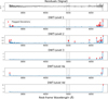 |
Fig. A.1 Top: Residuals of the fit in the three top panels of Fig. 3. Remaining panels: DWT coefficients and the flagged deviations (in red). Dashed lines delimit the region where the DWT flagged the residuals structure for the model recommendation. |
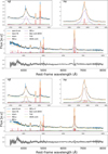 |
Fig. A.2 Comparison of the best-fit of a spectrum fitted with model-1 (three top panels), and best-fit with model-3, which was determined as the best model by the algorithm (three bottom panels). In both cases, the Hα and Hβ regions are zoomed, and the total fit and residuals are also shown. The main difference between both fits is the use of a second BELs component to fit the profile in the Hα and Hβ regions. |
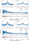 |
Fig. A.3 Comparison of the best-fit of a spectrum fitted with model-1 (three top panels), and best-fit with model-2, which was determined as the best model by the algorithm (three bottom panels). In both cases, the MgII, CIV regions are zoomed, and the total fit and residuals are also shown. The main difference between the fits is the use of a second BELs component that improves the fit in the MgII and CIV regions. |
Appendix B Algorithm and validators coincidence fraction
Here, we show all the results from the comparison between the algorithm and each validator recommendations. Table B.1 presents the results when considering all the objects. While Table B.2 shows the results for objects with z < 1.056, and Table B.3 for objects with z > 1.056. All these tables compare the different fc values. Also, the fractions for the complexity and simplicity-discrepancy are presented.
Coincidence between algorithm and validators for all objects.
Coincidence between algorithm and validators for objects with z < 1.056.
Coincidence between algorithm and validators for objects with z > 1.056.
Appendix C Synthetic spectra: Model recommendation
Here, we show the results obtained by the code for the synthetic spectra. We tabulated the best model from the code for each synthetic spectrum, grouping results by SN_MEDIAN_ALL.
Comparison of the synthetic spectrum model and code best model for SN_MEDIAN_ALL= 5.
Comparison of the synthetic spectrum model and code best model for SN_MEDIAN_ALL=10.
Comparison of the synthetic spectrum model and code best model for SN_MEDIAN_ALL=20.
Comparison of the synthetic spectrum model and code best model for SN_MEDIAN_ALL=30.
All Tables
Comparison of the synthetic spectrum model and code best model for SN_MEDIAN_ALL= 5.
Comparison of the synthetic spectrum model and code best model for SN_MEDIAN_ALL=10.
Comparison of the synthetic spectrum model and code best model for SN_MEDIAN_ALL=20.
Comparison of the synthetic spectrum model and code best model for SN_MEDIAN_ALL=30.
All Figures
|
Fig. 1 Distribution of the median S/N for low-redshift (top) and high-redshift (bottom) of the verification sample (orange), compared with the parent sample (blue). |
| In the text | |
|
Fig. 2 Redshift distribution for low-redshift (top) and high-redshift (bottom) sources of the verification sample (orange), compared with the parent sample (blue). |
| In the text | |
|
Fig. 3 Comparison of the best-fit of a spectrum fitted with model-1 (three top panels), and model-3 (three bottom panels), the last was the final result from the code. The Hβ and MgII regions are zoomed, and the total fit and residuals are also shown. The main difference between the two fits is the use of [OIII]winds. Dashed lines delimit the region where the DWT flagged the residuals structure (see Appendix A). All panels have the same arbitrary units on y-axis. |
| In the text | |
|
Fig. 4 Coincidence ratio between the algorithm and each validator. The mean coincidence across all validators is shown in markers, and the root-mean-squared scatter of coincidence ratios is represented by the error bars. Blue marks are for objects with z < 1.056 and orange marks for z > 1.056. The small markers (same color code) represent the random median fraction of coincidence obtained by the re-shuffling of the model choice by each validator. |
| In the text | |
|
Fig. 5 Fractional difference between the modeled flux, fm, and the synthetic flux, fs, for NELs. Colors indicate the SN_MEDIAN_AL of the synthetic spectrum, and marks indicate the S/N in the region of the emission line labeled on the y-axis. In the x-axis of the bottom panel the names of the synthetic models are presented: w00, w02, w05, and w10 are the reference for the percentage of [OIII]winds which are 0%, 20%, 50%, 100% of the [OIII] NELs. The “2bels” label is a reference to synthetic models with two BEls components. |
| In the text | |
|
Fig. 6 Fractional difference between the modeled-flux fm and the synthetic-flux fs for BELs. Colors indicate the SN_MEDIAN_AL of the synthetic spectrum, and marks indicate the S/N in the region of the emission line labeled on the y-axis. In the x-axis of the bottom panel, the labels are the same as in Fig. 5. |
| In the text | |
|
Fig. A.1 Top: Residuals of the fit in the three top panels of Fig. 3. Remaining panels: DWT coefficients and the flagged deviations (in red). Dashed lines delimit the region where the DWT flagged the residuals structure for the model recommendation. |
| In the text | |
|
Fig. A.2 Comparison of the best-fit of a spectrum fitted with model-1 (three top panels), and best-fit with model-3, which was determined as the best model by the algorithm (three bottom panels). In both cases, the Hα and Hβ regions are zoomed, and the total fit and residuals are also shown. The main difference between both fits is the use of a second BELs component to fit the profile in the Hα and Hβ regions. |
| In the text | |
|
Fig. A.3 Comparison of the best-fit of a spectrum fitted with model-1 (three top panels), and best-fit with model-2, which was determined as the best model by the algorithm (three bottom panels). In both cases, the MgII, CIV regions are zoomed, and the total fit and residuals are also shown. The main difference between the fits is the use of a second BELs component that improves the fit in the MgII and CIV regions. |
| In the text | |
Current usage metrics show cumulative count of Article Views (full-text article views including HTML views, PDF and ePub downloads, according to the available data) and Abstracts Views on Vision4Press platform.
Data correspond to usage on the plateform after 2015. The current usage metrics is available 48-96 hours after online publication and is updated daily on week days.
Initial download of the metrics may take a while.