| Issue |
A&A
Volume 707, March 2026
|
|
|---|---|---|
| Article Number | A47 | |
| Number of page(s) | 13 | |
| Section | Stellar structure and evolution | |
| DOI | https://doi.org/10.1051/0004-6361/202556826 | |
| Published online | 25 February 2026 | |
Asteroseismology of the ZZ Ceti star WD 1310+583 using the Transiting Exoplanet Survey Satellite
1
Konkoly Observatory, HUN-REN Research Centre for Astronomy and Earth Sciences, MTA Centre of Excellence H-1121 Budapest Konkoly Thege Miklós út 15-17, Hungary
2
Institute of Astronomy, KU Leuven Celestijnenlaan 200D B-3001 Leuven, Belgium
3
Instituto de Astrofísica de La Plata, IALP (CCT La Plata), CONICET-UNLP La Plata, Argentina
4
Grupo de Evolución Estelar y Pulsaciones. Facultad de Ciencias Astronómicas y Geofísicas, Universidad Nacional de La Plata Paseo del Bosque s/n (1900) La Plata, Argentina
5
Department of Physics, Gibbet Hill Road University of Warwick Coventry CV4 7AL, United Kingdom
6
Department of Astronomy, University of Texas at Austin Austin TX-78712, USA
7
McDonald Observatory Fort Davis TX-79734, USA
★ Corresponding author: This email address is being protected from spambots. You need JavaScript enabled to view it.
Received:
11
August
2025
Accepted:
12
January
2026
Abstract
Aims. By analysing the light curves of the ZZ Ceti star WD 1310+583, we aim to determine its pulsational frequencies and to give constraints on the main stellar parameters using asteroseismology.
Methods. We performed the Fourier analysis of the TESS light curves of WD 1310+583 and selected the possible pulsational modes. We also used spectroscopic data collected with the Cosmic Origins Spectrograph of the Hubble Space Telescope to give constraints for the asteroseismic analysis. We perform the latter with period-to-period fits using fully evolutionary white dwarf models.
Results. The star presented in this paper shows a particularly high number (41) of pulsational frequencies, which provides a potential opportunity for detailed asteroseismic investigations. We found a mean period spacing of ∼40.5 seconds, which allows us to state that the stellar mass of WD 1310+583 is larger than ∼0.57 M⊙. We also attempted an asteroseismological analysis by performing period-to-period fits, but we were unable to find a single statistically significant asteroseismological solution. We adopted a tentative solution consisting of a white dwarf model with M* = 0.632 M⊙, Teff = 11 702 K, and an asteroseismic distance d = 27.75−0.15+0.17 pc, which is significantly smaller than the one predicted by Gaia (d = 30.79 ± 0.2 pc). We also determined that the rotational period of our target is 1.18 d.
Key words: techniques: photometric / techniques: spectroscopic / stars: interiors / stars: oscillations / stars: individual: WD 1310+583 / white dwarfs
© The Authors 2026
 Open Access article, published by EDP Sciences, under the terms of the Creative Commons Attribution License (https://creativecommons.org/licenses/by/4.0), which permits unrestricted use, distribution, and reproduction in any medium, provided the original work is properly cited.
This article is published in open access under the Subscribe to Open model. This email address is being protected from spambots. You need JavaScript enabled to view it. to support open access publication.
1. Introduction
ZZ Ceti stars, also known as DAV stars, are pulsating white dwarfs with hydrogen-dominated atmospheres. These stars exhibit low-amplitude multiperiodic brightness variations caused by non-radial g-mode oscillations with periods ranging from 100 to 1500 seconds. These pulsations are driven by a combination of the κ − γ mechanism, operating within the partial ionisation zone of hydrogen (Dolez & Vauclair 1981; Winget et al. 1982), and the convective driving mechanism (Brickhill 1991; Goldreich & Wu 1999). With effective temperatures spanning 10 500–13 000 K, ZZ Ceti stars are confined to a well-defined region in the Hertzsprung–Russell diagram known as the ZZ Ceti instability strip.
As these stars cool across the instability strip, their pulsational properties vary systematically. Near the blue (hot) edge, they exhibit a lower number of pulsation modes with smaller amplitudes and shorter periods. Towards the red (cool) edge, the number of detectable modes increases, their amplitudes grow, and the pulsations become less stable, often showing amplitude and frequency variations on timescales of days to weeks (see e.g. Section 6 in Fontaine & Brassard 2008). Intriguingly, many cool ZZ Ceti stars also display episodic outbursts, characterised by brief and irregular increases in stellar brightness (see Bell et al. 2015, 2016, 2017; Bognár et al. 2023 and Hermes et al. 2015), which may provide insight into the interaction between pulsation and convection.
ZZ Ceti stars are invaluable astrophysical laboratories for investigating the physics of dense matter under extreme conditions. Their small size (approximately Earth-like) and high surface gravity (log g ∼ 8) result in strongly stratified atmospheres, where heavier elements settle below a hydrogen or helium layer due to gravitational separation. These characteristics make them ideal for asteroseismology, a technique that uses observed pulsation periods to infer the star’s internal structure, chemical composition, and rotational properties. Such studies contribute to understanding stellar evolution and the formation of compact objects (Winget & Kepler 2008; Fontaine & Brassard 2008; Althaus et al. 2010; Córsico et al. 2019; Córsico 2020).
Recent advances in space-based photometry, particularly with the Transiting Exoplanet Survey Satellite (TESS; Ricker et al. 2015), have revolutionised the study of ZZ Ceti stars. TESS provides high-precision, high-cadence observations, enabling detailed frequency analyses and the detection of new pulsation modes, even in stars previously deemed observationally challenging. This has opened new avenues for understanding the global properties of white dwarfs and the underlying physics driving their pulsations (Bell et al. 2019; Bognár et al. 2020).
The brightness variations of the ZZ Ceti star WD 1310+583 were independently discovered by Gentile Fusillo et al. (2018) and Bognár et al. (2018). The latter study presents photometric investigations conducted at the Konkoly Observatory (Hungary). Seven independent modes were identified on the basis of the datasets. In the study by Gentile Fusillo et al. (2018), two possible pulsation frequencies were published as a result of their analysis. The star has been independently suggested as a double degenerate source based on spectroscopic or hybrid (photometric, spectroscopic plus astrometric data) fits using ultraviolet (Gentile Fusillo et al. 2018) and optical (Munday et al. 2024) spectroscopy. Munday et al. (2024) found little radial velocity variability, indicating that the source is likely a wide double white dwarf binary star system.
In this paper, we focus on the TESS measurements of WD 1310+583. First, we analyse the spectroscopic data available on WD 1310+583, then we present the TESS datasets to identify the pulsation modes of this star. Using these findings, we estimate the period spacing to constrain the stellar mass of WD 1310+583 and attempt an asteroseismic investigation to constrain its global parameters and internal structure.
2. Spectroscopic analysis
In the following, we present the results of the system parameters of a double-degenerate fit to the spectra obtained on WD 1310+583 (TIC 157271533, G = 14.07 mag,  ,
,  ). At the time of writing, precise Gaia parallax measurements were not available to Gentile Fusillo et al. (2018), and the authors chose to fix the surface gravity of both stars to log g = 8.0 dex when producing the atmospheric parameters of the two stars. With that in mind and to obtain an improved spectroscopic solution to the ultraviolet data, we decided to refit their Hubble Space Telescope Cosmic Origins Spectrograph (HST COS) spectrum with new information at hand, utilising all-sky photometry and Gaia parallaxes to give absolute flux measurements.
We used the WD-BASS pipeline (Munday et al. 2024) with Pan-STARRS all-sky photometry (Chambers & Pan-STARRS Team 2018, filters grizy), the Sloan Digital Sky Survey (filters ugriz) DR16 (Ahumada et al. 2020), and the Gaia data release 3 (DR3) parallax of π = 32.48 ± 0.25 mas. We fitted the wavelength range of 1200–1930 Å, trimming the very low signal-to-noise data. We masked geocoronal lines between vacuum wavelengths 1206–1226 Å, 1295–1315 Å, and also within 1 Å of all entries supplied in the line list of Sahu et al. (2023) to ignore any potential undesired photospheric and/or interstellar flux contribution.
Synthetic spectra were obtained by interpolating the 3D local thermodynamic equilibrium grids of Tremblay et al. (2013, 2015) for DA white dwarfs, which are based on the line profiles of Tremblay & Bergeron (2009). The hotter star, which dominates the flux, has Balmer absorption lines and is clearly a DA, but the spectral class of the secondary star is unknown since it exhibits no unique spectral lines. Hence, the dimmer companion could be a helium-atmosphere DC, and in testing this DA plus DC combination, we interpolate synthetic spectra from Cukanovaite et al. (2021). The temperature, surface gravity, and radial velocity of the two stars and the parallax of the system were independent variables in the fitting. We used the mass–temperature–radius relationships from the hydrogen-rich (DA) and helium-rich (DC) evolutionary sequences of Bédard et al. (2020) to obtain stellar radii and calculate the luminosity of each star. Observations were scaled from an Eddington flux to an observed flux using the reciprocal of the parallax as the distance in parsecs, with an extinction coefficient of E(B − V) = AV/RV = 0.01/3.1 applied to redden the synthetic spectra (Gentile Fusillo et al. 2021). No spectrum normalisation was applied; the observed flux in physical units was fitted in both the HST COS spectrum and the all-sky photometry with a common parallax measurement to each dataset. A Gaussian prior was placed on the fitted parallax using the parallax, and the error reported in Gaia DR3.
However, as it turns out, we need to be careful with the automatic use of the Gaia parallax. The value of the parameter of the renormalised unit weight error (RUWE) for WD 1310+583 (Gaia DR3 1566603962760532736) is quite high: 16.315. This may also indicate the presence of a binary star system, as the RUWE parameter measures the goodness of an astrometric fit to the data (see e.g. Castro-Ginard et al. 2024). We checked the Gaia DR3 database (Gaia Collaboration 2022) and found that the parameter astrometric_excess_noise is 2.688 mas, the astrometric_excess_noise_sig is 4076, and the visibility_periods_used is 28. It strongly indicates that the ‘single-star’ astrometric model is not adequate: the high RUWE and, in particular, the large astrometric_excess_noise, together with its extreme significance, show that the assumed single-star model fails to explain many of the measurements. The most likely physical cause is photocentre motion (e.g. due to a close binary, an unresolved companion, or blending) or strong photometric variability that shifts the astrometric positions. Thus, the parallax may be inaccurate or partially biased (the formal parallax_error is likely too optimistic). We must bear in mind that it is not recommended to use the value of 32.48 mas automatically as an accurate distance estimate; however, this is currently the best-known estimate of the star’s distance. The visibility_periods_used = 28 shows that there was a sufficient number of observations, so the poor fit is not simply due to a small data sample; the deviation is real.
The best-fit solutions are shown in Figs. 1 and 2, respectively, while the physical parameters of the different solutions can be seen in Table 1. As in Gentile Fusillo et al. (2018), we conclude that a single star solution does not suffice to model WD 1310+583. The flux contributed by the companion in the ultraviolet is small, but the relative flux contribution from the companion becomes significant towards redder wavelengths. As such, the companion star serves as an extra flux contributor, and there is no way to decisively reveal its spectral type. For this reason, both combinations of DA plus DA and DA plus hydrogen-deficient DC are presented. Crucially, since the flux in the ultraviolet almost completely originates from the hotter object, the atmospheric parameters of the pulsating white dwarf are near identical across the two models, meaning that the unknown combination of DA plus DA or DA plus DC does not noticeably impact our astroseismetric analysis.
Physical parameters of different spectroscopic fits.
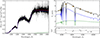 |
Fig. 1. Best-fitting solution for DA plus DA two-star model. Left panel: Fit to the HST COS spectrum. Right panel: Solution with photometric data. The synthetic flux from the hotter, pulsating white dwarf is shown in dashed blue while the flux from the cooler companion is shown in dashed green. In the left panel, the reduced spectrum is in grey, and the smoothed spectrum (across five data points) is in black. In the right panel, the synthetic flux in each filter is given as black circles, and the orange crosses are observed fluxes from the photometric surveys, with the percentage flux residual underneath. The total flux is in red on the left and black on the right for clarity. |
3. Light curve analyses of the TESS observations
TESS measured the star in 120-second short-cadence mode in these sectors: 15, 16, 22, 48, 49, 75, and 76. Measurements are also available in 20-second ultra-short cadence mode, but we did not see peaks above the Nyquist frequency of the 120-second measurements. So, we examined the 120-second measurements more closely.
First, we performed frequency analyses for sectors s15s16, s22, s48s49, and s75s76 using the photometric module of the Frequency Analysis and Mode Identification for Asteroseismology (FAMIAS) software package (Zima 2008). As seen, we treated the data of the neighbouring sectors jointly. For frequency analyses, we set the significance limit at 0.1% false alarm probability (FAP). We created a table of the observed peaks in the different sectors and considered the peaks that are approximately at the same frequency in the different datasets as the same frequency. The full list of detected frequencies can be found in the tables of Appendix B. After we identified the common frequencies and their amplitudes provided by the analyses, we calculated the amplitude-averaged period value for each frequency. A total of 67 frequencies were detected in the individual datasets. Based on pairwise frequency separations, 39 pairs with spacings smaller than 1.22 μHz were identified. Since all remaining pairs are separated by at least 2.70 μHz, we adopted 1.22 μHz as the threshold below which the frequencies were combined by means of a weighted average.
We also checked for the presence of linear combinations in each dataset. There are groups of peaks above about 700 s, and we considered the one with the highest amplitude as the representative frequency of the given frequency group. Table 2 summarises the journal of observations, while Appendix A lists the frequencies, periods, and amplitudes of the peaks detected by the analysis of the datasets from the different sectors. The comparison of the Fourier spectra of the different segments of the light curve is shown in Fig. 3.
 |
Fig. 3. Fourier spectra of different light curve segments. The horizontal black lines indicate the significance levels corresponding to a 0.1% FAP for each dataset. Amplitude variations are clearly visible from sector to sector. The vertical lines in each panel correspond to the frequencies listed in Appendix B. |
Journal of observations of WD 1310+583.
4. Rotational multiplets
The equation we used to calculate the rotation period of the star is as follows (see e.g. the Appendix in Winget et al. 1991):
 (1)
(1)
where k, l, and m are the radial order, horizontal degree, and azimuthal order of the non-radial pulsation mode, respectively. The coefficient Ck, l can be calculated as Ck, l ≈ 1/ℓ(ℓ + 1). This relation is valid for high-overtone (k ≫ ℓ) g-modes; Ω is the (uniform) rotational frequency.
Examining the frequencies listed in Appendix A reveals the presence of possible rotational triplet and doublet frequencies separated by approximately 5 and 10 μHz, respectively. The 10 μHz separations may correspond to triplets with 5 μHz frequency differences. A total of eight doublets were identified, as summarised in Fig. 4 and Table 3. Assuming that all are l = 1 modes and that the average frequency separation is 4.9 μHz, the star’s rotational period is calculated to be P = 1.18 d, considering Eq. (1). This value is in good agreement with the hour-to-day rotation periods typically observed in pulsating white dwarf stars; see, for example, Section 7 in Hermes et al. (2017).
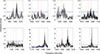 |
Fig. 4. Fourier spectra of possible rotational frequencies listed in Table 3. We note that we utilised pre-whitened Fourier spectra for the plots, as the lower-amplitude peaks become more clearly visible after pre-whitening. The horizontal blue lines indicate the significance levels corresponding to a 0.1% FAP for each dataset. |
Possible rotational doublet frequencies.
5. Period spacing tests
Here, our primary goal is to deepen our understanding of stellar structure, particularly the mass of the observed object. We note that the photometric and spectroscopic masses are in good agreement, as shown in Table B.1. of the following work: Calcaferro et al. (2024). The mean period spacing serves as an indicator of the stellar mass. We conducted several tests, as follows: using a subset of the periods listed in Appendix A, we searched for a characteristic period spacing using Kolmogorov-Smirnov (K-S; Kawaler 1988) and inverse variance (I-V; O’Donoghue 1994) significance tests. In the K-S test, the quantity Q represents the probability that the observed periods are randomly distributed. A characteristic period spacing in the period spectrum would manifest itself as a minimum in Q. Meanwhile, in the I-V test, a maximum indicates the presence of a constant period spacing. Another widely recognised approach to identifying a characteristic spacing value is performing a Fourier analysis on a Dirac comb constructed directly with periods (e.g. Winget et al. 1991; Handler et al. 1997).
Fig. 5 shows the results of applying the statistical tests to a subset of 11 periods detected in WD 1310+583. These periods are marked with an asterisk in Appendix A. The three tests reveal a clear period spacing of 40.58 s, which can be associated with modes that have ℓ = 1. A spacing of ∼20 seconds is also observed in the three tests. This corresponds to the subharmonic of the spacing (ΔΠ/2). Using a linear least-squares fit to the identified dipole modes, we derive a mean period spacing of ΔΠℓ = 1 = 40.51 s (see Fig. 6). To robustly estimate the associated uncertainty, we adopted the error-propagation method described by Uzundag et al. (2023), which is based on the approach of Uzundag et al. (2021). This method involves generating 1000 random permutations of the observed periods, in each case assigning a value of m ∈ { − 1, 0, +1} for triplets (and m ∈ { − 2, −1, 0, +1, +2} for quintuplets) to all detected modes. Then each set is adjusted to the intrinsic m = 0 component assuming rotational splitting, and a new linear fit is performed. The uncertainty in the mean period spacing is taken as the standard deviation of the resulting distribution of best-fit slopes, yielding  s. The residuals of the observed periods relative to this mean period spacing (lower panel of Fig. 6) clearly reveal deviations consistent with mode trapping signatures in the pulsation spectrum of WD 1310+583. The discovery of the period spacing ΔΠℓ = 1 allows the harmonic degree ℓ = 1 to be assigned to the 11 periods that make up the sequence, allowing strong constraints to fits of individual periods to be placed (see Section 6.2).
 |
Fig. 5. Results of inverse variance (I-V, black), Kolmogorov-Smirnov (K-S, blue), and Fourier Transform (F-T, red) statistical tests applied to subset of 11 periods marked with asterisks in Appendix A. The three tests point to the existence of a period spacing of 40.58 s in WD 1310+583, which can be associated to ℓ = 1 modes. The presence of the subharmonic of this spacing at ∼20 seconds is also apparent. |
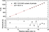 |
Fig. 6. Upper panel: Linear least-squares fit to 11 periods of WD 1310+583 marked with asterisks in Appendix A. The derived period spacing from this fit is ΔΠℓ = 1 = 40.51 s. Lower panel: Residuals of the period distribution relative to the mean period spacing, revealing signals of mode trapping in the period spectrum of WD 1310+583. Modes with a consecutive radial order are connected with thin black lines. |
In summary, we first used rotational multiplets to identify the most secure modes. These identifications then served as priors when we searched for the asymptotic period-spacing pattern. We applied this procedure consistently. The two methods are not in conflict; they are complementary.
6. Asteroseismology
All of our efforts to determine the independent pulsation modes were to provide these modes for the asteroseismic analysis of the star presented in the following sections. We begin with the determination of the stellar mass using the identified period spacings and then proceed to present the results of the asteroseismic period-to-period fits.
6.1. The stellar mass of WD 1310+583 as predicted by the observed period spacing
A practical approach to estimating the stellar mass of pulsating WD (white dwarf) stars involves comparing the observed period spacing (ΔΠ) with the average of the calculated period spacings ( ) (Córsico et al. 2019). The average is determined using the formula
  , where ‘forward’ period spacing (ΔΠk) is defined as ΔΠk = Πk + 1 − Πk (with k representing the radial order) and n is the number of periods computed that fall within the range of observed periods. It is important to note that this method for determining stellar mass depends on the spectroscopic effective temperature, and the results are inevitably influenced by the uncertainties associated with Teff. The method mentioned leverages the fact that, in general, the period spacing of pulsating WD stars is mainly influenced by stellar mass and effective temperature, with only a minor dependence on the thickness of the He envelope for DBV stars or the O/C/He envelope for GW Vir stars (see e.g. Tassoul et al. 1990). However, this technique cannot be directly applied to DAV stars for mass estimation, as the period spacing in these stars is influenced by M★, Teff, and the mass of the H envelope MH, with similar sensitivity, leading to multiple combinations of these three parameters that yield the same period spacing. Therefore, we can only provide a possible range of stellar masses for WD 1310+583 based on the period spacing.
We calculated the mean of the period spacings for ℓ = 1, denoted as  , employing the LP-PUL pulsation code (Córsico & Althaus 2006), in terms of the effective temperature across all the stellar masses considered and the thicknesses of the H envelope (see Table 4 of Uzundag et al. 2023). The analysed period range was established between 300 and 1600 seconds, encompassing the typical periods observed in the target star WD 1310+583. The effective temperature of WD 1310+583 according to this work (see Sect. 2) is Teff = 11 660 ± 163 K on average. However, there are other measurements of Teff for this DAV star in the literature, such as Teff = 10 131 ± 260 K (Leggett et al. 2018), Teff = 10 313 ± 111 K (O’Brien et al. 2024), Teff = 11 617 ± 70 K (Gentile Fusillo et al. 2018), and Teff = 11 600 ± 200 K (Munday et al. 2024). In particular, the value of Teff derived in the present study is almost the same as the values derived by Gentile Fusillo et al. (2018) and Munday et al. (2024).
As there is no definitive effective temperature measurement available for this star, we used multiple estimates to cover the possible range of Teff. The results are illustrated in Fig. 7, showing  for various stellar masses (specified at the top right corner of each panel), represented by curves with different thicknesses corresponding to the diverse values of MH. To enhance clarity, we only labelled the extreme H-envelope thickness values for each stellar mass, using thick and thin black curves. The position of WD 1310+583, marked by a small circle with error bars, was examined with three spectroscopic effective temperature values: Teff = 10 131 ± 260 K (Leggett et al. 2018), Teff = 10 313 ± 111 K (O’Brien et al. 2024), representative of most of the Teff determinations, which point to low effective temperatures, and Teff = 11 660 ± 163 K (this paper), along with a period spacing of ΔΠ = 40.51 ± 0.14 s.
Upon analysis of the plot, we infer that, based on the period spacing and Teff, the stellar mass of WD 1310+583 likely falls between 0.570 M⊙ (with a thick H envelope of log(MH/M★) = − 3.82) and 0.877 M⊙ (with a very thin H envelope of log(MH/M★) = − 9.29) if the effective temperature is high (green dot in Fig. 7). In contrast, if the effective temperature of WD 1310+583 is lower (as indicated by the red and blue dots in Fig. 7), then the stellar mass would probably exceed 0.705 M⊙ with a thick envelope of H (log(MH/M★) = − 4.45). In summary, based on the period spacing and effective temperature, the stellar mass of WD 1310+583 would be higher than ∼0.57 M⊙.
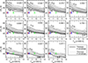 |
Fig. 7. Average of computed dipole (ℓ = 1) period spacings, |

6.2. Asteroseismic period-to-period fits
In this section, we try to find an evolutionary model that best matches the theoretical periods with the individual pulsation periods detected for WD 1310+583. The quality of the fit is assessed by evaluating the quality function defined as follows:
![Mathematical equation: $$ \begin{aligned} \sigma ^2(M_{\star },M_H,T_{\rm eff}) = \frac{1}{N} \sum _{i=1}^{N} \mathrm {min}[(\Pi _i^{O}-\Pi _k^{th})^2]. \end{aligned} $$](/articles/aa/full_html/2026/03/aa56826-25/aa56826-25-eq11.gif) (2)
(2)
Here, N represents the number of detected modes, ΠiO are the observed periods, and Πkth are the theoretically computed periods (where k is the radial order). The best-fitting model, if it exists, is chosen by identifying the minimum value of σ2.
We use the same grid of CO-core WD models as in Uzundag et al. (2023), which contemplates evolutionary sequences of stellar masses in the range 0.525 ≤ M★/M⊙ ≤ 0.877, with effective temperature 10 000 K ≤ Teff ≤ 13 000 K, and varying the total hydrogen content −9 ≲ log(MH/M★)≲ − 4. For the period-to-period fit, we examined the frequency spectrum of WD 1310+583 and used the confirmed triplets and the consecutive overtones derived as ℓ = 1 as input priors; see Appendix A and Table 3. We considered the central components (with m = 0), specifically the eight observed periods (793.4, 837.6, 873.8, 919.3, 953.6, 997.1, 1038.4, and 1078.4 s), which were assigned ℓ = 1 for the analysis.
In Fig. 8 we show the value of the inverse of the squared quality function for our models, in the range of effective temperatures of interest. With solid lines, we highlight the quality function for the models that best match the observed periods, as indicated by the maximum in the curve. The two models represented by the maxima of the dashed blue (cyan) curves next to the solid curves were discarded because of their hot (cold) effective temperatures. The three best-fit models highlighted represent only marginally better fits than other models, which prevents us from considering them as seismic measurements of the properties of WD 1310+583. Indeed, the three individual highest peaks are not statistically compelling enough for their parameters to be worth discussing as properties of this star. In view of this, from now on we limit ourselves to describing the properties of tentative seismological solutions for WD 1310+583.
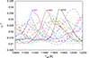 |
Fig. 8. Inverse of squared quality as function σ defined in Eq. (2) in terms of effective temperature. Solid (dashed) lines represent the value for the selected (discarded) models (see Table 4).
Table 4. Parameters of the best-fit models. |
The most important stellar parameters of our tentative asteroseismic models are shown in Table 4. Given the Teff values obtained in this work, which considers the binary nature of this system, we focus our analysis in the vicinity of Teff ∼ 11 600 K. Based on our results, it is more likely that WD 1310+583 would have a thick H-envelope. However, the more massive solution exhibits a significant discrepancy with our spectroscopic determination of log g and the Gaia distance; therefore, we reject this model as a possible solution.
Always bearing in mind that none of these solutions is formally statistically significant, we can consider model 3 as a possible description of the structure of WD 1310+583 since its mass aligns with the results of the mean period spacing analysis and provides the best agreement between the theoretical and observed periods. Our tentative asteroseismological model is characterised by total H- and He-content of 4.46 × 10⁻⁶ M* and 1.75 × 10⁻² M*, respectively, and a luminosity of L/L⊙ = 0.25 × 10⁻². We derived the internal uncertainties in the most important stellar parameters from the model grid resolution χM★ = 0.028 M⊙, χTeff = 70 K, χlog g = 0.05, χL★/L⊙ = 2 × 10⁻⁴, and χR★/R⊙ = 1.2 × 10⁻⁴.
Based on the stellar parameters derived from our tentative representative model, we estimate the asteroseismic distance of WD 1310+583. From the derived effective temperature and the logarithm of surface gravity, we calculated the absolute magnitude in the Gaia G band (D. Koester, personal communication). For the model with a mass of 0.632 M⊙, we find that the absolute magnitude is MG = 11.85 mag. From the apparent magnitude obtained by the Gaia DR3 Archive1 for WD 1310+583 (mG = 14.07 mag), we obtain an asteroseismic distance of  pc. We found that our distance is appreciably smaller compared to the Gaia distance (Bailer-Jones et al. 2021), which reports d = 30.79 ± 0.2 pc.
7. Discussion
WD 1310+583 was one of the targets observed from the Konkoly Observatory as part of a survey aimed at discovering new pulsating white dwarf stars potentially detectable by TESS (see Bognár et al. 2018). This study presented observations obtained over eight nights, complemented by a preliminary asteroseismic analysis of the star. They identified 17 significant frequencies, seven of which were found to be independent pulsation modes, as also summarised in the introduction of this paper. Preliminary asteroseismic modelling was performed for six of these modes using the White Dwarf Evolution Code (WDEC; see Bischoff-Kim et al. 2008). Four of the six modes were also detected in the TESS data, within the limits of the observational uncertainties.
The preliminary asteroseismic analysis presented by Bognár et al. (2018) aimed to constrain the stellar mass, the effective temperature, and the mass of the hydrogen layer. Adapting the observed periods for six modes and assuming that at least four of them, including the dominant one, correspond to dipole modes (ℓ = 1), the following parameters were derived: M* = 0.74 M⊙, Teff = 11 600 K, and −log MH = 4.0. This mass is approximately 0.1 M⊙ higher than that obtained from fully evolutionary models (this work), while the hydrogen layer mass is roughly two orders of magnitude higher. However, the effective temperatures derived from the two modelling approaches are quite similar (11 600 K vs 11 702 K).
Bognár et al. (2018) also reported possible values of the rotational frequency splittings and the corresponding rotation periods. The stellar rotation period could be either 5 h or 1.3 d. It should be noted that the latter value is very close to the 1.18 d obtained from the TESS measurements.
The comparison between our asteroseismic results and previous analyses highlights the typical challenges in reconciling spectroscopic and seismological determinations of white dwarf parameters, particularly for DAVs (see Calcaferro et al. 2024). In this case, the asteroseismic mass derived from WDEC modelling exceeds the spectroscopic mass by about 0.1 M⊙, a discrepancy that falls within the range commonly observed in pulsating DAs. Such differences may arise from systematic uncertainties that affect both methods. Spectroscopic parameters (Teff, log g) depend on the atmosphere models adopted and the treatment of line broadening and convection, which significantly influence the Balmer line profiles (Saumon et al. 2022). As shown by Fuchs (2017), unaccounted for systematics such as imperfect flux calibration, extinction corrections, or low signal-to-noise ratios can introduce biases in Teff and log g, thereby affecting the derived masses. On the other hand, asteroseismic masses depend sensitively on mode identification and on the adopted model grids and internal chemical stratification profiles (De Gerónimo et al. 2018, 2017). For WD 1310+583, the assumption that most detected modes correspond to ℓ = 1 may have influenced the stellar structure parameters of our tentative asteroseismological model, since even a small number of ℓ = 2 modes can alter the inferred mass and thickness of the hydrogen layer.
We also emphasise that, as Fig. 8 clearly shows, our selected model is only a tentative solution. The best-fit models are only marginally better fits than the other models, which means that the models presented in Table 4 are not statistically significant, so we cannot find a robust seismological solution. Although the star shows a rich pulsation spectrum with robustly identified modes, this does not mean that we can find a representative model, highlighting the need for improvements on the modelling side and the asteroseismological method employed, as also discussed in Calcaferro et al. (2024).
Our analysis of WD 1310+583 exemplifies the broader trend observed among DAVs, where the spectroscopic mass may overestimate or underestimate the seismological mass depending on the interplay of uncertainties in both approaches. The degeneracy between the core and envelope structure in high-overtone g-modes (see Montgomery et al. 2003; Giammichele et al. 2017) also contributes to potential ambiguities in the derived stellar parameters, even when several independent pulsation periods are available. In particular, the number of detected modes is not necessarily indicative of the reliability of the seismological solution; rather, it is their distribution in radial order and the degree of mode trapping that determine the diagnostic power of the dataset.
8. Summary
This study presents an asteroseismic investigation of the ZZ Ceti star WD 1310+583. A prerequisite for asteroseismic modelling is the identification of the star’s normal pulsation modes. These modes were derived from 120-second cadence photometric data obtained with TESS, supplemented by relevant parameters available in the literature.
Additional constraints were provided by spectroscopic analysis, based on data collected with the Cosmic Origins Spectrograph onboard the Hubble Space Telescope. We also examined the possible presence of rotationally split multiplets.
By means of an asteroseismic analysis, we derived a suggestive asteroseismological model characterised by the following physical parameters: M* = 0.632 M⊙, Teff = 11 702 K, the stellar mass being compatible with the predictions of the period spacing (M★ ≳ 0.6 M⊙). The corresponding asteroseismic distance (27.75 pc) is smaller compared to the geometric distance inferred from Gaia astrometry (30.79 pc).
Continued operation of the TESS mission will enable not only similarly detailed case studies, but also ensemble analyses of white dwarf pulsators and the discovery of new compact variables. Here, we demonstrate the high scientific value of studying white dwarf variables with TESS, and the continuation of these observations would be of great benefit to the white dwarf community.
Acknowledgments
The authors thank the anonymous referee for constructive comments and recommendations on the manuscript. The authors acknowledge Michael H. Montgomery (Department of Astronomy, University of Texas at Austin; McDonald Observatory, Fort Davis) for the useful early discussions. The authors also acknowledge Mukremin Kilic (Homer L. Dodge Department of Physics and Astronomy, University of Oklahoma), Antoine Bedard (Department of Physics, University of Warwick) and Detlev Koester (Institut für Theoretische Physik und Astrophysik, Universität Kiel) for their helpful discussion. Zs.B. and Á.S. acknowledge the financial support of the KKP-137523 ‘SeismoLab’ Élvonal grant of the Hungarian Research, Development and Innovation Office (NKFIH). M.U. gratefully acknowledges support from the Research Foundation Flanders (FWO) through a Junior Postdoctoral Fellowship (grant agreement No: 1247624N). This paper includes data collected with the TESS mission, obtained from the MAST data archive at the Space Telescope Science Institute (STScI). Funding for the TESS mission is provided by the NASA Explorer Programme. STScI is operated by the Association of Universities for Research in Astronomy, Inc., under NASA contract NAS 5–26555.
References
- Ahumada, R., Allende Prieto, C., Almeida, A., et al. 2020, ApJS, 249, 3 [NASA ADS] [CrossRef] [Google Scholar]
- Althaus, L. G., Córsico, A. H., Isern, J., & García-Berro, E. 2010, A&ARv, 18, 471 [NASA ADS] [CrossRef] [Google Scholar]
- Bailer-Jones, C. A. L., Rybizki, J., Fouesneau, M., Demleitner, M., & Andrae, R. 2021, VizieR On-line Data Catalog: I/352 [Google Scholar]
- Bédard, A., Bergeron, P., Brassard, P., & Fontaine, G. 2020, ApJ, 901, 93 [Google Scholar]
- Bell, K. J., Hermes, J. J., Bischoff-Kim, A., et al. 2015, ApJ, 809, 14 [NASA ADS] [CrossRef] [Google Scholar]
- Bell, K. J., Hermes, J. J., Montgomery, M. H., et al. 2016, ApJ, 829, 82 [CrossRef] [Google Scholar]
- Bell, K. J., Hermes, J. J., Montgomery, M. H., et al. 2017, ASP Conf. Ser., 509, 303 [NASA ADS] [Google Scholar]
- Bell, K. J., Córsico, A. H., Bischoff-Kim, A., et al. 2019, A&A, 632, A42 [NASA ADS] [CrossRef] [EDP Sciences] [Google Scholar]
- Bischoff-Kim, A., Montgomery, M. H., & Winget, D. E. 2008, ApJ, 675, 1505 [NASA ADS] [CrossRef] [Google Scholar]
- Bognár, Z., Kalup, C., Sódor, Á., Charpinet, S., & Hermes, J. J. 2018, MNRAS, 478, 2676 [Google Scholar]
- Bognár, Z., Kawaler, S. D., Bell, K. J., et al. 2020, A&A, 638, A82 [NASA ADS] [CrossRef] [EDP Sciences] [Google Scholar]
- Bognár, Z., Sódor, Á., Clark, I. R., & Kawaler, S. D. 2023, A&A, 674, A204 [NASA ADS] [CrossRef] [EDP Sciences] [Google Scholar]
- Brickhill, A. J. 1991, MNRAS, 251, 673 [NASA ADS] [Google Scholar]
- Calcaferro, L. M., Córsico, A. H., Uzundag, M., et al. 2024, A&A, 691, A194 [NASA ADS] [CrossRef] [EDP Sciences] [Google Scholar]
- Castro-Ginard, A., Penoyre, Z., Casey, A. R., et al. 2024, A&A, 688, A1 [NASA ADS] [CrossRef] [EDP Sciences] [Google Scholar]
- Chambers, K.& Pan-STARRS Team 2018, AAS Meet. Abstr., 231, 102.01 [Google Scholar]
- Córsico, A. H. 2020, Front. Astron. Space Sci., 7, 47 [Google Scholar]
- Córsico, A. H., & Althaus, L. G. 2006, A&A, 454, 863 [NASA ADS] [CrossRef] [EDP Sciences] [Google Scholar]
- Córsico, A. H., Althaus, L. G., Miller Bertolami, M. M., & Kepler, S. O. 2019, A&ARv, 27, 7 [Google Scholar]
- Cukanovaite, E., Tremblay, P.-E., Bergeron, P., et al. 2021, MNRAS, 501, 5274 [NASA ADS] [CrossRef] [Google Scholar]
- De Gerónimo, F. C., Althaus, L. G., Córsico, A. H., Romero, A. D., & Kepler, S. O. 2017, A&A, 599, A21 [NASA ADS] [CrossRef] [EDP Sciences] [Google Scholar]
- De Gerónimo, F. C., Althaus, L. G., Córsico, A. H., Romero, A. D., & Kepler, S. O. 2018, A&A, 613, A46 [NASA ADS] [CrossRef] [EDP Sciences] [Google Scholar]
- Dolez, N., & Vauclair, G. 1981, A&A, 102, 375 [NASA ADS] [Google Scholar]
- Fontaine, G., & Brassard, P. 2008, PASP, 120, 1043 [NASA ADS] [CrossRef] [Google Scholar]
- Fuchs, J. T. 2017, Ph.D. Thesis, University of North Carolina, Chapel Hill [Google Scholar]
- Gaia Collaboration 2022, VizieR On-line Data Catalog: I/355 [Google Scholar]
- Gentile Fusillo, N. P., Tremblay, P. E., Jordan, S., et al. 2018, MNRAS, 473, 3693 [NASA ADS] [CrossRef] [Google Scholar]
- Gentile Fusillo, N. P., Tremblay, P. E., Cukanovaite, E., et al. 2021, MNRAS, 508, 3877 [NASA ADS] [CrossRef] [Google Scholar]
- Giammichele, N., Charpinet, S., Brassard, P., & Fontaine, G. 2017, A&A, 598, A109 [NASA ADS] [CrossRef] [EDP Sciences] [Google Scholar]
- Goldreich, P., & Wu, Y. 1999, ApJ, 511, 904 [NASA ADS] [CrossRef] [Google Scholar]
- Handler, G., Pikall, H., O’Donoghue, D., et al. 1997, MNRAS, 286, 303 [NASA ADS] [CrossRef] [Google Scholar]
- Hermes, J. J., Montgomery, M. H., Bell, K. J., et al. 2015, ApJ, 810, L5 [Google Scholar]
- Hermes, J. J., Gänsicke, B. T., Kawaler, S. D., et al. 2017, ApJS, 232, 23 [Google Scholar]
- Kawaler, S. D. 1988, IAU Symp., 123, 329 [Google Scholar]
- Leggett, S. K., Bergeron, P., Subasavage, J. P., et al. 2018, ApJS, 239, 26 [NASA ADS] [CrossRef] [Google Scholar]
- Liebert, J., Bergeron, P., & Holberg, J. B. 2005, ApJS, 156, 47 [NASA ADS] [CrossRef] [Google Scholar]
- Montgomery, M. H., Metcalfe, T. S., & Winget, D. E. 2003, MNRAS, 344, 657 [NASA ADS] [CrossRef] [Google Scholar]
- Munday, J., Pelisoli, I., Tremblay, P. E., et al. 2024, MNRAS, 532, 2534 [NASA ADS] [CrossRef] [Google Scholar]
- O’Brien, M. W., Tremblay, P. E., Klein, B. L., et al. 2024, MNRAS, 527, 8687 [Google Scholar]
- O’Donoghue, D. 1994, MNRAS, 270, 222 [Google Scholar]
- Ricker, G. R., Winn, J. N., Vanderspek, R., et al. 2015, J. Astron. Telesc. Instrum. Syst., 1, 014003 [Google Scholar]
- Sahu, S., Gänsicke, B. T., Tremblay, P.-E., et al. 2023, MNRAS, 526, 5800 [Google Scholar]
- Saumon, D., Blouin, S., & Tremblay, P.-E. 2022, Phys. Rep., 988, 1 [NASA ADS] [CrossRef] [Google Scholar]
- Tassoul, M., Fontaine, G., & Winget, D. E. 1990, ApJS, 72, 335 [Google Scholar]
- Tremblay, P. E., & Bergeron, P. 2009, ApJ, 696, 1755 [Google Scholar]
- Tremblay, P. E., Ludwig, H. G., Steffen, M., & Freytag, B. 2013, A&A, 559, A104 [NASA ADS] [CrossRef] [EDP Sciences] [Google Scholar]
- Tremblay, P. E., Gianninas, A., Kilic, M., et al. 2015, ApJ, 809, 148 [NASA ADS] [CrossRef] [Google Scholar]
- Uzundag, M., Vučković, M., Németh, P., et al. 2021, A&A, 651, A121 [NASA ADS] [CrossRef] [EDP Sciences] [Google Scholar]
- Uzundag, M., De Gerónimo, F. C., Córsico, A. H., et al. 2023, MNRAS, 526, 2846 [NASA ADS] [CrossRef] [Google Scholar]
- Winget, D. E., & Kepler, S. O. 2008, ARA&A, 46, 157 [Google Scholar]
- Winget, D. E., van Horn, H. M., Tassoul, M., et al. 1982, ApJ, 252, L65 [NASA ADS] [CrossRef] [Google Scholar]
- Winget, D. E., Nather, R. E., Clemens, J. C., et al. 1991, ApJ, 378, 326 [NASA ADS] [CrossRef] [Google Scholar]
- Zima, W. 2008, CoAst, 155, 17 [NASA ADS] [Google Scholar]
Appendix A: Frequency, period, and amplitude values determined from the TESS datasets.
Frequency, period, and amplitude values determined from the TESS datasets.
Appendix B: Frequencies, periods, and amplitudes of the detected signals in the datasets of the different sectors.
Results of analysis of sector s15s16 dataset.
Results of analysis of sector s22 dataset.
Results of analysis of sector s48s49 dataset.
Results of analysis of sector s75s76 dataset.
All Tables
All Figures
|
Fig. 1. Best-fitting solution for DA plus DA two-star model. Left panel: Fit to the HST COS spectrum. Right panel: Solution with photometric data. The synthetic flux from the hotter, pulsating white dwarf is shown in dashed blue while the flux from the cooler companion is shown in dashed green. In the left panel, the reduced spectrum is in grey, and the smoothed spectrum (across five data points) is in black. In the right panel, the synthetic flux in each filter is given as black circles, and the orange crosses are observed fluxes from the photometric surveys, with the percentage flux residual underneath. The total flux is in red on the left and black on the right for clarity. |
| In the text | |
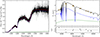 |
Fig. 2. As for Fig. 1 but for a DA plus DC two-star model. See Sect. 2 for more details. |
| In the text | |
|
Fig. 3. Fourier spectra of different light curve segments. The horizontal black lines indicate the significance levels corresponding to a 0.1% FAP for each dataset. Amplitude variations are clearly visible from sector to sector. The vertical lines in each panel correspond to the frequencies listed in Appendix B. |
| In the text | |
|
Fig. 4. Fourier spectra of possible rotational frequencies listed in Table 3. We note that we utilised pre-whitened Fourier spectra for the plots, as the lower-amplitude peaks become more clearly visible after pre-whitening. The horizontal blue lines indicate the significance levels corresponding to a 0.1% FAP for each dataset. |
| In the text | |
|
Fig. 5. Results of inverse variance (I-V, black), Kolmogorov-Smirnov (K-S, blue), and Fourier Transform (F-T, red) statistical tests applied to subset of 11 periods marked with asterisks in Appendix A. The three tests point to the existence of a period spacing of 40.58 s in WD 1310+583, which can be associated to ℓ = 1 modes. The presence of the subharmonic of this spacing at ∼20 seconds is also apparent. |
| In the text | |
|
Fig. 6. Upper panel: Linear least-squares fit to 11 periods of WD 1310+583 marked with asterisks in Appendix A. The derived period spacing from this fit is ΔΠℓ = 1 = 40.51 s. Lower panel: Residuals of the period distribution relative to the mean period spacing, revealing signals of mode trapping in the period spectrum of WD 1310+583. Modes with a consecutive radial order are connected with thin black lines. |
| In the text | |
|
Fig. 7. Average of computed dipole (ℓ = 1) period spacings, |
| In the text | |
|
Fig. 8. Inverse of squared quality as function σ defined in Eq. (2) in terms of effective temperature. Solid (dashed) lines represent the value for the selected (discarded) models (see Table 4).
Table 4. Parameters of the best-fit models. |
| In the text | |
Current usage metrics show cumulative count of Article Views (full-text article views including HTML views, PDF and ePub downloads, according to the available data) and Abstracts Views on Vision4Press platform.
Data correspond to usage on the plateform after 2015. The current usage metrics is available 48-96 hours after online publication and is updated daily on week days.
Initial download of the metrics may take a while.