| Issue |
A&A
Volume 707, March 2026
|
|
|---|---|---|
| Article Number | A71 | |
| Number of page(s) | 16 | |
| Section | Numerical methods and codes | |
| DOI | https://doi.org/10.1051/0004-6361/202556878 | |
| Published online | 03 March 2026 | |
Efficient black hole seed formation in low-metallicity and dense stellar clusters with implications for JWST sources
1
Astronomisches Rechen-Institut, Zentrum für Astronomie, University of Heidelberg,
Mönchhofstrasse 12-14,
69120
Heidelberg,
Germany
2
Nicolaus Copernicus Astronomical Center, Polish Academy of Sciences,
Bartycka 18,
00-716
Warsaw,
Poland
3
Department of Physics, New York University Abu Dhabi,
PO Box
129188
Abu Dhabi,
UAE
4
Center for Astrophysics and Space Science (CASS), New York University Abu Dhabi,
PO Box
129188,
Abu Dhabi,
UAE
5
Dipartimento di Fisica, Sapienza Università di Roma,
Piazzale Aldo Moro 5,
00185
Rome,
Italy
6
Departamento de Astronomía, Facultad Ciencias Físicas y Matemáticas, Universidad de Concepción, Av. Esteban Iturra s/n Barrio Universitario,
Casilla 160-C,
Concepción,
Chile
7
Departamento de Astronomía, Universidad de Chile,
Casilla 36-D,
Santiago,
Chile
8
National Astronomical Observatories and Key Laboratory of Computational Astrophysics, Chinese Academy of Sciences,
20A Datun Rd., Chaoyang District,
Beijing
100012,
China
9
Kavli Institute for Astronomy and Astrophysics, Peking University,
Yiheyuan Lu 5, Haidian Qu,
100871
Beijing,
China
10
OzGrav: The ARC Centre of Excellence for Gravitational Wave Discovery,
Hawthorn,
VIC
3122,
Australia
11
Centre for Astrophysics and Supercomputing, Department of Physics and Astronomy,
John Street, Hawthorn,
Victoria
3122,
Australia
12
Gran Sasso Science Institute,
Viale F. Crispi 7,
67100
L’Aquila,
Italy
13
Physics and Astronomy Department Galileo Galilei, University of Padova,
Vicolo dell’Osservatorio 3,
35122
Padova,
Italy
14
INFN – Laboratori Nazionali del Gran Sasso,
67100
L’Aquila, (AQ),
Italy
15
INAF – Osservatorio Astronomico d’Abruzzo, Via M. Maggini snc,
64100
Teramo,
Italy
16
Max-Planck-Institut für Astronomie,
Königstuhl 17,
69117
Heidelberg,
Germany
★ Corresponding authors: This email address is being protected from spambots. You need JavaScript enabled to view it.
; This email address is being protected from spambots. You need JavaScript enabled to view it.
Received:
15
August
2025
Accepted:
16
December
2025
Abstract
Context. Recent observations with the James Webb Space Telescope (JWST) have revealed the presence of young massive clusters (YMCs) as building blocks of the first galaxies during the first billion years of the Universe. They are not only important constituents of the galaxies, but also potential birthplaces of very massive stars (VMSs) and black hole (BH) seeds.
Aims. In this paper, we investigate whether runaway stellar collisions in extremely dense clusters inevitably lead to the formation of VMSs and BH seeds. We focus on clusters with initial half-mass densities of ρh ≳ 108 M⊙ pc−3 at very low metallicity (Z = 10−4), using idealized initial conditions that assume a fully formed, gas-free, monolithic stellar system. Our goal is to follow their early internal evolution and quantify the efficiency of collisional growth.
Methods. We use NBODY6++GPU and MOCCA, including the latest updates of the single stellar evolution (SSE) and binary stellar evolution (BSE), along with specific routines to handle the formation, growth through collisions, and dynamical evolution of VMSs.
Results. Our direct N-body and Monte Carlo simulations show that VMSs form rapidly and unavoidably through repeated collisions, reaching final masses of ~5 × 10³ to 4 × 10⁴ M⊙, before collapsing into BH seeds of similar mass in less than 4 Myr. These results confirm the existence of a critical mass scale at which collisional growth becomes highly efficient, enabling the formation of VMSs and potentially intermediate-mass BHs.
Conclusions. We identify a critical mass–density threshold beyond which clusters undergo runaway collisions, leading to efficient BH-seed formation. For YMCs detected with JWST, we expect efficiencies up to ~10%, corresponding to BH masses as large as 105 M⊙. We predict a BH mass–cluster mass scaling relation of log(MBH / M⊙) = −0.76 + 0.76 log(M / M⊙). Frequent VMS formation in this regime may also provide a natural explanation for the strong nitrogen enrichment observed in some high-redshift galaxies.
Key words: methods: numerical / stars: massive / globular clusters: general
© The Authors 2026
 Open Access article, published by EDP Sciences, under the terms of the Creative Commons Attribution License (https://creativecommons.org/licenses/by/4.0), which permits unrestricted use, distribution, and reproduction in any medium, provided the original work is properly cited.
This article is published in open access under the Subscribe to Open model. This email address is being protected from spambots. You need JavaScript enabled to view it. to support open access publication.
1 Introduction
Recently, the James Webb Space Telescope (JWST) has observed young massive clusters (YMCs) in the early Universe, challenging current models of cosmic evolution. These stellar systems are extremely massive and dense, and their presence at high redshift implies that they must have formed within the first few hundred million years after the Big Bang (Vanzella et al. 2022a,b, 2023; Adamo et al. 2024; Mowla et al. 2024; Messa et al. 2026). Three main routes have been suggested as a possible explanation for the formation of massive and compact stellar systems. (i) collapse of gas in high-density environments. This process can lead to a high formation efficiency (SFE) of up to 80% (Menon et al. 2023; Somerville et al. 2025), (ii) merger-driven starbursts, via gas-rich dwarf galaxy mergers (Renaud et al. 2015; Lahén et al. 2020a,b, 2025), and (iii) turbulent fragmentation within gas filaments and clumps, whereby supersonic turbulence within molecular clouds causes hierarchical fragmentation into dense clumps, each of which can independently collapse to form bound clusters (Longmore et al. 2014; Klessen & Glover 2016; Polak et al. 2024). The YMCs have short formation and emergence timescales, typically a few million years (Longmore et al. 2021; Linden et al. 2024; Polak et al. 2024; Lahén et al. 2025), much shorter than those of open clusters, which can span tens of millions of years (Wang et al. 2021). The formation rate correlates with cluster density and mass; denser and more massive clusters emerge faster due to stronger gravitational binding and more effective feedback-driven gas removal by stars (Adamo et al. 2023; Grudić et al. 2023).
These highly dense stellar environments are ideal places for runaway collisions to occur and form a very massive star (VMS; Spitzer & Saslaw 1966; Spitzer & Stone 1967; Sanders 1970; Lee 1987; Quinlan & Shapiro 1990; Gürkan et al. 2004; Freitag et al. 2006b,a; Giersz et al. 2015; Vergara et al. 2023, 2024, 2025; Rantala & Naab 2025; Rantala et al. 2025) and also are suitable places for chemical self-enrichment (Vink 2018). These primordial dense stellar systems and their capability to form VMSs can be a possible explanation for other mysteries observations by the JWST, such as the high nitrogen-to-oxygen ratio in galaxies at high redshift (Charbonnel et al. 2023), which is around four times larger than in the solar vicinity (Cameron et al. 2023). Some examples of these galaxies with high nitrogen abundances are GN-z11 at redshift 10.6 (Bouwens et al. 2010; Tacchella et al. 2023; Nagele & Umeda 2023; Maiolino et al. 2024), CEERS-1019 at z = 8.679 (Larson et al. 2023; Marques-Chaves et al. 2024), and the most distant one to date, MOM-z14 at z = 14.44 (Naidu et al. 2025).
To explain the formation of VMSs and supermassive black holes (SMBHs), several scenarios have been proposed in the literature (Rees 1978, 1984). One prominent scenario involves the remnants of Population III (Pop III) stars, which form in metal-free clouds and accrete mass onto their cores (Bond et al. 1984; Omukai & Nishi 1998; Madau & Rees 2001; Volonteri et al. 2003; Tan & McKee 2004; Ricarte & Natarajan 2018; Mestichelli et al. 2024; Liu et al. 2024; Reinoso et al. 2025; Solar et al. 2025). The Pop III stars under rapid rotation are potential sources of nitrogen enrichment (Tsiatsiou et al. 2024; Nandal et al. 2024). Alternatively, the direct collapse of gas clouds (Loeb & Rasio 1994; Begelman et al. 2006; Lodato & Natarajan 2006; Chon & Omukai 2025), possibly through a quasi-star phase (Begelman 2010), has been suggested as another viable pathway. Stellar dynamics have been proposed as a possible pathway (Portegies Zwart et al. 1999; Portegies Zwart & McMillan 2002; Reinoso et al. 2018, 2020; Alister Seguel et al. 2020; Vergara et al. 2021, 2023, 2024, 2025).
The early attempts to explain the high luminosities observed in galactic centers relied on analytical models. Spitzer & Saslaw (1966); Spitzer & Stone (1967) demonstrated that luminosities of ~1043 erg s−1 can arise in dense star clusters of 108 M⊙ within a radius of ~0.1 pc. Similarly, Sanders (1970) showed that VMSs could form in stellar systems with short relaxation times. The VMS formation via collisions was first predicted using Fokker-Planck models, which indicated that a massive star naturally forms at the cluster core due to the deep gravitational potential (Lee 1987). Later, Quinlan & Shapiro (1990) proposed that dense galactic nuclei could host stars with masses of thousands of solar masses, potentially seeding SMBHs. Monte Carlo simulations by Gürkan et al. (2004) revealed that dense clusters undergo core collapse faster than the lifetime of a massive star, enabling sustained mass growth before collapse. In particular, clusters with over a million stars exhibit high collision rates, facilitating the formation of ~103 M⊙ stars that may collapse into intermediate-mass black holes (IMBHs; Freitag et al. 2006a,b; Giersz et al. 2015). Direct N-body simulations have also produced massive stars of hundreds of solar masses (Portegies Zwart et al. 1999, 2004). The first million-particle N-body simulation, DRAGON (Wang et al. 2016), marked a significant milestone. Subsequent studies, including the DRAGON-II simulations by Arca Sedda et al. (2023, 2024b,a), have investigated the formation of IMBHs in star clusters with central densities of approximately 105 M⊙ pc−3. Escala (2021) further argued that stellar systems become prone to global instability, and thus conducive to massive object formation, if their average collision timescale is comparable to or shorter than their age, and discussed that primordial stellar clusters are ideal candidates to undergo such a physical process. Vergara et al. (2023) has demonstrated with equal-mass star models that above a certain critical mass, defined when the average collision timescale is equal to their age, collapse becomes inevitable and massive objects can form in clusters with central densities up to 1010 M⊙ pc−3. This finding was expanded to different stellar systems, including not only nuclear stellar clusters (NSCs), but also globular clusters (GCs) and ultracompact dwarf galaxies (UCDs), covering different initial conditions, stellar initial mass functions (IMFs), and evolutionary paths (Vergara et al. 2024). Using the critical mass framework, Liempi et al. (2025) reproduced the observed mass distribution of NSCs and SMBHs with semi-analytical models. Recently, Vergara et al. (2025) conducted one of the most computationally intensive million-particle simulations to date, with a central density of >107 M⊙ pc−3, forming an IMBH of >5 × 10⁴ M⊙ within 5 Myr. Another scenario involves relativistic clusters, whereby stellar black holes (BH) dynamics may facilitate SMBH formation (Shapiro & Teukolsky 1985; Lupi et al. 2014; Kroupa et al. 2020; Gaete et al. 2024; Bamber et al. 2025).
In this study, we focus on the early internal evolution of clusters once assembled, rather than on their gas-rich, multi-million-yearformation phase. We adopt idealized initial conditions that assume a fully formed, gas-free stellar system, capturing the high-density, collision-driven conditions potentially relevant to the most compact YMCs seen with JWST. Within this framework, we investigate whether runaway stellar collisions unavoidably lead to the formation of VMSs and the subsequent growth of seed BHs. This paper is structured as follows: Section 2 presents the methodology and introduces the initial conditions. Section 3 presents the results. Finally, Section 4 provides a summary of the conclusions along with a discussion of theoretical aspects.
2 Methodology
For this study, we performed simulations with the direct N-body code NBODY6++GPU and MOCCA1. Both codes have been widely compared (Giersz et al. 2008, 2015; Heggie 2014; Wang et al. 2016; Madrid et al. 2017; Kamlah et al. 2022b; Vergara et al. 2025), showing excellent agreement in terms of stellar dynamics and individual stellar properties. Both share stellar and binary evolution recipes based on the single stellar evolution (SSE) and binary stellar evolution (BSE) population synthesis codes (Hurley et al. 2000, 2002, 2005) and updates to them by Banerjee et al. (2020), Kamlah et al. (2022b), Spurzem & Kamlah (2023), and Vergara et al. (2025).
2.1 NBODY6++GPU
NBODY6++GPU is a high-precision direct N-body code (Spurzem 1999; Wang et al. 2015; Spurzem & Kamlah 2023). It includes several algorithms to solve the stellar dynamics such as the Kustaanheimo-Stiefel regularization, an algorithm to solve close encounters and to form binaries (Stiefel & Kustaanheimo 1965), the chain regularization (Mikkola & Aarseth 1989, 1993), the fourth-order Hermite integrator scheme with hierarchical block time-steps (Hut et al. 1995; Makino & Aarseth 1992; Makino 1999), the Ahmad-Cohen neighbour scheme which spatially splits the stellar hierarchy to speed up computational calculations (Ahmad & Cohen 1973), and parallelization and acceleration that allow large number of particles, using GPU (Wang et al. 2015); for example, Wang et al. (2016), Arca Sedda et al. (2023, 2024b,a), and Vergara et al. (2025). It enables realistic simulations of star clusters. The algorithms behind the treatment of the stellar dynamics are explained in more detail in the review article by Spurzem & Kamlah (2023) on collisional stellar systems.
2.2 MOCCA
MOCCA is a code for simulating the evolution of realistic star clusters (Giersz et al. 2013; Hypki & Giersz 2013). It is based on the Monte Carlo method developed by Hénon (1971), which was subsequently improved by Stodolkiewicz (1982, 1986) and Giersz (2001). This method combines the particle-based approach of direct N-body simulations with a statistical treatment of two-body relaxation, allowing for efficient computation of the long-term dynamical evolution of spherically symmetric star clusters. MOCCA includes treatments for important physical processes that drive cluster evolution, including SSE and BSE as in N-body, the effects of a galactic tidal field, and the direct integration of strong dynamical encounters using the FEWBODY code (Fregeau et al. 2004) for scattering experiments.
2.3 Initial conditions
Our models assume fully formed, gas-free, monolithic clusters in order to probe the post-assembly, collision-dominated regime potentially relevant to the most compact YMCs observed with JWST. We used McLuster to generate the initial conditions for the N-body and MOCCA codes. We modeled five isolated clusters using a King density profile (King et al. 1968), with W0 = 6, including a Kroupa IMF (Kroupa 2001) with the range M* = 0.08–150 M⊙. We varied the number of stars as N = 5 × 10⁴, 105, 2 × 10⁵, 5 × 10⁵, 7.5 × 10⁵, we did not include primordial binaries, the cluster half-mass radius varied as Rh = 0.005, 0.01, 0.05 pc and the absolute metallicity was 10−4 (see Table 1). Models R005N750k and R005N500k were motivated by some of the most recent observations with JWST at high redshift, which revealed dense stellar systems with effective radii of ≲1 pc and masses on the order of 105–106 M⊙ (Vanzella et al. 2022a, 2026; Adamo et al. 2024; Messa et al. 2026). We emphasize that our initial models are extremely dense, having central half-mass densities roughly two orders of magnitude higher than those inferred for observed high-redshift clusters. However, by the end of the simulations (at ~4 Myr), their resulting surface densities become broadly comparable to the observed values (see Section 3.3). Models R001N250k, R001N100k, and R0005N50k are proof-of-concept runs at even higher densities. To keep the problem tractable, we used compact, lower-N clusters, which still allowed us to probe much shorter dynamical timescales. Although less massive than many JWST-detected YMCs, our models reach comparable or higher densities, which set the collisional regime. The resulting efficiencies and scalings should thus be taken as indicative of more massive systems at similar densities, while the exact outcomes may depend on additional processes. We neglected residual gas, ongoing star formation, and primordial binaries; gas could further accelerate runaway growth through drag, while binaries might delay it via heating. However, at such high central densities, the velocity dispersion in the core is large enough that most soft binaries would be efficiently disrupted, while the harder ones would likely be driven to merge rapidly through frequent dynamical interactions (Miller & Davies 2012; Stone et al. 2017). For these reasons, binary heating is unlikely to prevent or significantly delay the early core collapse in our models. At the extreme densities explored here, collisions dominate, and our results provide upper limits on the efficiency of VMS and seed BH formation in the most compact clusters.
In Fig. 1, we display the initial half-mass density ρh of the star cluster model, evaluated at the initial half-mass radius rh, versus the initial star number N. We include a color bar to represent the average logarithm of the half-mass radius. In this figure, we compare the average values of different sets of simulations and the code used, including the direct N-body codes, shown as circle symbols in plot representing initial conditions from Portegies Zwart et al. (1999), Fujii & Portegies Zwart (2013), Katz et al. (2015), Wang et al. (2015), Mapelli (2016), Sakurai et al. (2017), Reinoso et al. (2018), Panamarev et al. (2019), Reinoso et al. (2020), Di Carlo et al. (2020), Rastello et al. (2021), Rizzuto et al. (2021), Banerjee (2021), Gieles et al. (2021), Vergara et al. (2021), Kamlah et al. (2022a), Rizzuto et al. (2023), Vergara et al. (2023), Arca Sedda et al. (2023, 2024b,a), and Vergara et al. (2025), which are P+99, F+13, K+15, W+15, M+16, S+17, R+18, P+19, R+20, D+20, R+20, R+21, B+21, G+21, V+21, K+22, R+23, V+23, AS+23, and V+25, respectively. Simulations with Monte-Carlo codes are shown as square symbols in the plot representing initial conditions from Askar et al. (2017), Rodriguez et al. (2019), Kremer et al. (2020), Maliszewski et al. (2022), and Rodriguez et al. (2022), which are A+17, R+19, K+20, M+22, and R+22, respectively. Finally hybrid N-body simulations with diamond symbols in the plot represent the initial conditions from Wang et al. (2021), Wang et al. (2022), and Wang et al. (2024), which are labeled as W+21, W+22, and W+24, respectively. The latter use the PETAR code (Wang et al. 2020), which is classified as a hybrid N-body code, because it combines direct particle-particle interactions with accelerated tree-based approximations. In particular we include the following key benchmarks: the first N-body simulation with one million bodies, known as the dragon simulation, with an average density of ρh ~ 104 M⊙ pc−3 (Wang et al. 2015); and the DRAGON-II simulations by Arca Sedda et al. (2023, 2024b,a) exhibiting densities of ρh = 1.3 × 10⁴ to 6.9 × 10⁵ M⊙ pc−3 for a particle range of N = 1.2 × 10⁵–106, with 10–33% of primoridal binaries, and forming BHs with masses around 60–350 M⊙. Additionally, Vergara et al. (2023) simulated compact clusters with equal-mass stars, reaching densities up to 1010 M⊙ pc−3 with fewer particles ranging from N ~ 103–104, forming massive objects of 60–68 000 M⊙. The recent one-million-particle simulation by Vergara et al. (2025) achieved the highest-recorded density to date ρh = 6.9 × 10⁷ M⊙ pc−3, and produced an IMBH with a mass of 50 000 M⊙. In the present work, we report simulations that reach even higher central densities, of up to ρh ~ 1010 M⊙ pc−3, which places our models relative to prior N-body and Monte Carlo initial conditions and highlights the extreme density regime we are targeting.
Initial conditions of the cluster models.
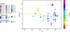 |
Fig. 1 Initial half-mass density ρh, computed at the initial half-mass radius rh, is expressed as a function of the initial number of stars N. The figure has been reproduced from Arca Sedda et al. (2023, 2024b,a) and adapted to include a color bar with the logarithm of the average half-mass radius. We include other simulations and the new ones presented in this paper. |
3 Results
In this section, we present the results from the simulations of the initial models described in Sect. 2.3. We focus on the post-assembly evolution of fully formed, gas-free clusters in the extreme density regime (see Fig. 1), investigating their stellar dynamics, stellar evolution, and the efficiency of VMS and BH seed formation through runaway collisions. Each cluster was evolved up to 4 Myr, which for the more extended models spans a few initial relaxation times, for the most compact ones a few tens, and in all cases far exceeds the crossing time. This ensures that collisional runaway and mass segregation are well captured within the simulations (see Fig. B.1), with each run extending beyond the time needed for the VMS to evolve into an IMBH.
3.1 Dynamical evolution of stellar clusters
In this subsection, we analyze the evolution of the cumulative mass that escapes from the star clusters, the number of collisions, and the Lagrangian radii at 90, 50, 30, 10, 5 and 1%. The dynamics of stellar clusters are governed by key timescales, the average collision timescale (tcoll) which determines the frequency of stellar collisions and is expressed as ![Mathematical equation: $\[t_{coll}=\sqrt{R / G M\left(n \Sigma_{0}\right)^{2}}\]$](/articles/aa/full_html/2026/03/aa56878-25/aa56878-25-eq1.png) (Binney & Tremaine 2008), where R and M are the radius and the mass of the cluster, G is the gravitational constant, Σ0 is the effective cross-section and n is the number density within the half mass radius; and the relaxation timescale (trx) which describes the time for the cluster to reach equilibrium via gravitational interactions and follows trx = (0.1N/ ln (γN))tcross, where
(Binney & Tremaine 2008), where R and M are the radius and the mass of the cluster, G is the gravitational constant, Σ0 is the effective cross-section and n is the number density within the half mass radius; and the relaxation timescale (trx) which describes the time for the cluster to reach equilibrium via gravitational interactions and follows trx = (0.1N/ ln (γN))tcross, where ![Mathematical equation: $\[t_{cross}=\sqrt{R^{3} / G M}, \gamma\]$](/articles/aa/full_html/2026/03/aa56878-25/aa56878-25-eq2.png) is the Coulomb logarithm and N the number of stars (Binney & Tremaine 2008). From an analysis of observational data of NSCs, Escala (2021) proposed that comparing relaxation and collision timescales (trx, tcoll) with the age of a cluster (τ) determines whether collisions drive massive central object formation. Vergara et al. (2023) tested this using equal-mass star simulations, defining a critical mass when tcoll = τ to quantify the transition to collision-dominated evolution, leading to a critical mass of Mcrit = R7/3 (4πM*/3Σ0τG1/2)2/3, marking the onset of runaway stellar collisions when M/Mcrit ~ 0.1.
is the Coulomb logarithm and N the number of stars (Binney & Tremaine 2008). From an analysis of observational data of NSCs, Escala (2021) proposed that comparing relaxation and collision timescales (trx, tcoll) with the age of a cluster (τ) determines whether collisions drive massive central object formation. Vergara et al. (2023) tested this using equal-mass star simulations, defining a critical mass when tcoll = τ to quantify the transition to collision-dominated evolution, leading to a critical mass of Mcrit = R7/3 (4πM*/3Σ0τG1/2)2/3, marking the onset of runaway stellar collisions when M/Mcrit ~ 0.1.
In Fig. 2, we present the dynamical regime of stellar systems in terms of their half-mass radius and total mass. We illustrate the interplay between both key dynamical timescales, tcoll and trelax, which fall within the range 1 Myr ≤ τ ≤ 10 Gyr, highlighting different dynamical regimes: pink for two-body relaxation and gray for stellar collisions. The lower limit of τ = 1 Myr corresponds approximately to the typical timescale for early cluster formation and the lifetimes of the most massive stars, while the upper limit of τ = 10 Gyr is set by the Hubble time, representing the maximum age over which stellar systems can dynamically evolve. The gray-shaded region is where collisions are significant throughout the lifetime of the cluster, starting practically from the very beginning in post-collapse evolution. It also illustrates the concept of a critical mass that increases steeply with radius, meaning that compact systems are more prone to entering the collisional regime. On the other hand, the pink-shaded region is where stellar systems are more likely to evolve by relaxation and avoid collisions (Escala 2021; Vergara et al. 2023). The overlapping region, dark pink, where both the two-body relaxation time and the stellar collision times fall between 1 Myr and 10 Gyr, suggests that systems in this region are neither extremely dense nor extremely diffuse, but instead evolve significantly through both two-body relaxation and direct stellar collisions over cosmic timescales. The shaded pink and black areas present an asymmetry that highlights that relaxation is a more widespread and efficient process across a wide range of stellar systems, whereas frequent stellar collisions require much more compact and dense conditions.
We also include the initial half-mass radii and masses of our models (see Table 1) connected with an arrow to the final half-mass radii and masses of the respective models R00SN750k, R005N500k, R001N250k, R001N100k and R0005N50k, which are denoted by yellow, cyan, orange, green, and magenta star symbols, respectively (empty for initial and full for final properties). Our models lie between the dotted lines (when tcoll and trx are equal to τ = 4 Myr). The models R001N250k, R001N100k, and R0005N50k fall within the collision-dominated regime. Their proximity to the dotted line indicates that they will experience several collisions, leading to the early formation (<4 Myr) of a massive central object (Escala 2021; Vergara et al. 2023). In contrast, the R005N750k and R005N500k models lie in the dark pink region. These systems are also susceptible to collisions but will proceed through a more typical relaxation process. While the models within the gray-shaded area display highly stochastic behavior, those in the dark pink region evolve in a less chaotic manner.
The expansion of a star cluster is a well-known phenomenon, driven primarily by internal dynamical processes but also by external tidal forces (see e.g. Fujii & Portegies Zwart 2016). Over time, the escape rate from the cluster increases significantly as binary interactions become more frequent, indicating that stellar escapes are primarily driven by energy generated in these encounters. This gradual loss of stars, known as cluster evaporation, leads to a decrease in the mass of the cluster (see Appendix D). Additionally, binary stars can inject energy into the system through three-body encounters, further enhancing the expansion of the cluster. Our models evolve rightward and downward in parameter space as a result of expansion driven by mass loss through escapers.
In Fig. 3, we display the evolution of two models, R0005N50k and R005N750k, the densest star cluster and the most massive star cluster, respectively. We present the temporal evolution of the Lagrangian radii. The top panel shows the temporal evolution of model R005N750k; the Lagrangian radius at 1% shows a sharp decline at the start of the simulation due to mass segregation, followed by a decrease in the 5% after 1 Myr, while the 10% shows a slight initial decrease before it evaporates smoothly and begins to decline slightly later. The 30 and 50% radii have an initial expansion that then continues steadily until the end. In contrast, the 90% radius grows consistently throughout the simulation. The bottom panel shows that the 1 and 5% radii decrease sharply at the beginning of the simulation, while the 10% begins its decline slightly later. Eventually, all three curves overlap, since the VMS controls the radii; the 30% and 50% radii have an initial more rapid expansion then smoothly continue expanding to the end, while the 90% grows drastically at the beginning and then remains almost constant for the remainder of the simulation. Both models exhibit a steep initial decline in their innermost regions (1%), although in R0005N50k, the 1 and 5% curves overlap at the start of the simulation; in R005N750k, the 5% radius decreases more gradually after 1 Myr. In R00SN750k, the 10% curve expands smoothly before a late decline, while in R0005N50k, it drops off earlier and merges with the innermost curves. The 30 and 50% curves expand in both cases; however, in the R0005N50k model, it is faster than in R00SN750k. Finally, R0005N50k shows a more abrupt initial growth in the 90% curve, which then stabilizes, unlike the constant growth observed in R005N750k. These differences suggest that the initial conditions significantly influence the dynamical evolution of the system. Model R005N750k has a less violent behavior than model R0005N50k; this less violent process helps to retain more stars within the cluster, which is a reserve of stars that eventually can fall to the center, contributing to the growth of the VMS due to the constant stellar bombardment. On the other hand, R0005N50k presents a stochastic evolution, whereby several stars segregate almost immediately to the center; however, the low number of particles does not allow the VMS to be more massive.
In Fig. 4, we show the time evolution of the cumulative escaping mass normalized by the initial cluster mass (top panel) and the cumulative number of collisions involving the VMS, normalized by the initial number of stars (bottom panel) for our five cluster models. The solid lines represent the results of direct N-body simulations, while the dashed lines show the results of Monte Carlo simulations. In the top panel, we observe that clusters with fewer particles (e.g., model R0005N50k) exhibit higher escape mass fractions compared to those with more particles (e.g., model R005N750k). These lower-N clusters are also denser, which leads to more dramatic dynamical evolution: the inner regions rapidly collapse at the beginning of the simulation, triggering multiple collisions. Additionally, enhanced three-body interactions increase the number of stars escaping from the system (see bottom panel in Fig. 3). In contrast, clusters with more particles (but lower density) show a lower ratio of cumulative escape mass normalized by the initial cluster mass. These systems exhibit a lower ratio of the number of binary collisions to the initial number of particles; thus, the evaporation process is weaker (see Appendix D). The cumulative mass of escapers is 12 371 M⊙, 17 252 M⊙, 27 173 M⊙, 24 431 M⊙, and 31 133 M⊙ in N-body simulations, and 13 380 M⊙, 18 888 M⊙, 44 610, M⊙ 45 640 M⊙, and 29 984 M⊙ in Monte Carlo simulations for models R0005N50k, R001N100k, R001N250k, R005N500k, and R00SN750k, respectively.
In the bottom panel, models R0005N50k, R001N100k and R001N250k with the smallest size (Rh ≤ 0.01 pc) and lowest particle number show the highest collision rate, consistent with its dense and rapidly collapsing core. The Monte Carlo and N-body results agree reasonably well, though the Monte Carlo simulations tend to slightly underestimate the number of collisions (see Appendix B for details). Models R005N500k and R005N750k, representing the most massive and extended clusters, show the lowest per-star collision rates due to longer relaxation times, with similar trends in both simulation approaches. Denser clusters present higher ratios, however, since the collision counts are normalized by the initial number of stars, the ratio does not directly reflect the absolute number of collisions. The total number of collisions with VMS is 1135, 1571, 5956, 5100, 10 919 in N-body and 716, 404, 1182, 2859, 4417 in Monte Carlo simulations for models for models R0005N50k, R001N100k, R001N250k, R005N500k, and R005N750k, respectively. Although the Monte Carlo method yields fewer total collisions, these typically involve more massive stars (>100 M⊙), while the N-body simulations produce more frequent collisions involving lower-mass stars (<1 M⊙). For more discussion on this distinction, refer to Appendix C.
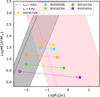 |
Fig. 2 Initial and final masses and half-mass radii of the clusters. The dotted lines represent when the timescales (tcoll and trx) are equal to τ = 4 Myr. The shaded regions indicate the parameter space where the respective timescales fall within the range 1 Myr ≤ τ ≤ 10 Gyr, highlighting different dynamical regimes: pink for two-body relaxation and gray for stellar collisions. Our clusters R0005N50k, R001N100k, R001N250k, R005N500k, and R005N750k evolve for 3.73, 3.81, 3.64, 3.80, and 3.87 Myr, respectively. We show their initial conditions with empty symbols and the final conditions with filled symbols, connected by arrows. |
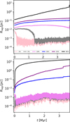 |
Fig. 3 Lagrangian radii calculated from the initial mass of the cluster for the 90, 70, 50, 30, 10, and 1% of the enclosed mass of model R005N750k (top) and model R0005N50k (bottom). |
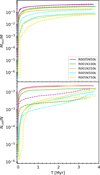 |
Fig. 4 Time evolution of the cumulative escaping mass normalized by the initial cluster mass (top) and the number of collisions with the most massive object normalized by the initial particle numbers (bottom). The solid lines are for N-body simulations and the dashed lines are for MOCCA ones. |
3.2 Black hole formation efficiency
In this subsection, we analyze the BH masses and their formation efficiency ϵBH = (1 + Mf/MBH)−1, which is defined as the fraction of mass between the final mass of the cluster and the total BH mass. This efficiency quantifies the fraction of the total stellar mass available in the system that eventually ends up in the BH, through stellar collisions, making it possible to explore the transition from a star-dominated cluster (ϵBH ~ 0) to a BH-dominated cluster (ϵBH ~ 1) as a function of the ratio of the initial mass to the critical mass M/Mcrit.
Fig. 5 shows the mass evolution of the VMS and BH seeds, in our five cluster models. Solid lines indicate the results from direct N-body simulations, while dashed lines represent Monte Carlo simulations. In models R005N750k and R005N500k, both simulation types show a steep increase in mass with time, with Monte Carlo results reaching slightly higher values. Model R001N250k shows an early rapid increase in mass, with a plateau around 1 Myr for both methods, presenting a slightly higher mass in N-body simulation. Models R001N100k and R0005N50k reach a much lower total mass, with their growth mostly flattening after ≲0.5 Myr. The VMS forms earlier in less massive clusters, whereas in more massive clusters the VMS is more massive. Its growth is prolonged because of continued stellar bombardment. The formation of the BH seeds is delayed in clusters with larger particle numbers, as the larger stellar reservoir allows the VMS to rejuvenate more frequently, postponing its collapse. All curves show a characteristic drop when the BH seed is formed, corresponding to a loss of mass of 10% due to neutrino emission (Fryer et al. 2012; Kamlah et al. 2022b). We summarize the masses’ milestones for each model in Table 2. Despite being more compact due to computational limits, our simulated clusters host BH seeds ranging from a few thousand to tens of thousands of solar masses. Observing stellar systems that host BHs remains challenging, as the high core brightness often obscures the possible presence of a black hole. Nonetheless, strong evidence consistent with an IMBH with a mass of at least 8200 M⊙ was recently identified at the center of ω Cen, based on observations of stars moving faster than the expected central escape velocity of the cluster (Häberle et al. 2024).
In Fig. 6, we show the BH formation efficiency (ϵBH) as a function of the ratio of the initial mass to the critical mass M/Mcrit. The dashed black line represents an asymmetrical sigmoid function fit to both numerical simulations and observational data collected in Vergara et al. (2024). The observational data include diverse stellar systems such as NSCs (e.g., Georgiev et al. 2016; Neumayer et al. 2020), GCs (e.g., Harris 1996; Lützgendorf et al. 2013), and UCDs (e.g., Afanasiev et al. 2018; Voggel et al. 2018). The numerical data are from different N-body simulations performed using different codes, such as, NBODY6 (Aarseth 1999), NBODY6++GPU (Wang et al. 2015; Spurzem & Kamlah 2023), and BIFROST (Rantala et al. 2023). These simulations include different density profiles, such as those of Plummer (1911) and King (1966), as well as different IMFs, including Salpeter (1955), Scalo (1986), and Kroupa (2001), and also models with equal-mass stars. To quantify the uncertainty in our nonlinear fit, we employed a bootstrap resampling method. By repeatedly resampling the original data with replacement 1000 times and refitting the asymmetric sigmoid curve, we generated a set of fit curves. From this set, we derived empirical confidence intervals at the uncertainties of the 1σ, 2σ, and 3σ regions, calculating the corresponding percentiles of the predicted curves at each point. These confidence bands provide a robust, nonparametric estimate of the uncertainty in the fit model that naturally accounts for the noise and variability of the observed and simulated data collected in Vergara et al. (2024). The form of the fit is given by, ϵBH = (1 + exp [−k(log (M/Mcrit) − x0)])a, where k = 4.63 controls the steepness of the transition, x0 = 4 sets its location, and a = −0.1 determines the smoothness of the function.
The efficiency starts to increase when the initial mass approaches the critical mass, i.e., M/Mcrit ~ 0.1 (Vergara et al. 2024). We include our models. Those with higher densities exhibit the highest BH formation efficiency, even though their BH seeds are the lightest. Since ϵBH is a function between the BH mass and the remnant stellar mass, models with higher density experience more escapers, leaving the cluster with less stellar mass at the end of the simulation. However, systems with more particles but lower densities show a lower efficiency. However, they experience more collisions, leading to heavier BH seeds compared to denser systems. We also include the simulation from Vergara et al. (2025), which aligns well with the models presented in this work and the trend observed in Vergara et al. (2024). The density plays an important role in the onset of collisions and VMS formation (see Fig. 1); however it is also limited by the number of stars available to sink to the center, so the formation of a VMS and subsequently a BH seed is influenced by these two parameters. In Table 3, we summarize the BH seed masses, the formation time and the BH formation efficiency (ϵBH).
Time of the milestones of the VMS mass formed.
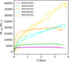 |
Fig. 5 Time evolution of the mass growth of VMSs that collapse into BH seeds. Solid lines represent N-body simulations and dashed lines MOCCA ones. |
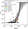 |
Fig. 6 BH formation efficiency as a function of the ratio of initial cluster mass to critical mass. The figure has been reproduced from Vergara et al. (2024); we fit an asymmetric sigmoid function, represented by the dashed black line. The shaded gray bands represent the confidence intervals estimated by bootstrap resampling: the darker, middle, and lighter gray bands correspond to the 1σ, 2σ, and 3σ uncertainty regions. These intervals quantify the uncertainty in the fit curve, arising from data variability. We added the simulation from Vergara et al. (2025) and the simulations from this work. |
Comparison of BH seed properties and formation efficiencies across models.
3.3 Comparison with JWST observations
In this subsection, we place the final structural properties of our simulated clusters in the context of observed young star clusters (YSCs) in the local Universe (Brown & Gnedin 2021) and the recently reported compact stellar systems observed with JWST at high redshift (Vanzella et al. 2022a,b, 2023; Mowla et al. 2024; Adamo et al. 2024). Our aim is to show that the clusters produced in our simulations fall within the broad range of sizes and surface densities covered by these observations, keeping in mind that our models are only ~4 Myr old, and therefore have had limited time to expand.
On the left side of Fig. 7, we show the final effective radii and masses of our simulated clusters (star symbols), together with the YSC catalogue from Brown & Gnedin (2021) and the recently reported YMCs with the JWST. We computed the effective radius as the projected radius enclosing half of the total cluster luminosity at the end of the simulation. The observed YSCs span masses of 104–106, M⊙ and effective radii from ~0.1 to > 10, pc, while the high-redshift YMCs occupy a similar mass range but can be significantly more compact. Our simulated clusters, with masses of 104–106, M⊙ and final effective radii of ~0.1–1 pc, lie somewhat to the left of most observed systems. This behavior is expected because the clusters are still very young and have not yet had time to undergo substantial expansion. This is broadly consistent with observational examples in which the youngest and most massive clusters tend to remain more compact (Brown & Gnedin 2021).
On the right side of Fig. 7, we show the stellar surface densities as a function of cluster mass. We computed the surface density by summing the mass enclosed within the effective radius and dividing by ![Mathematical equation: $\[\pi R_{\text {eff}}^{2}\]$](/articles/aa/full_html/2026/03/aa56878-25/aa56878-25-eq3.png) . The simulated clusters span Σ ~ 103–106, M⊙ pc−2, overlapping with both local YSCs and high-redshift YMCs. In our models, the more massive clusters exhibit higher surface densities and slightly older ages within the ~4 Myr simulation window, which is broadly in line with trends seen in observational samples (Brown & Gnedin 2021). High-redshift YMCs show a wide range of masses and ages, including extremely compact systems at z ~ 8–10 (Mowla et al. 2024; Adamo et al. 2024), and our simulated clusters lie at the younger and lower-mass end of this distribution.
. The simulated clusters span Σ ~ 103–106, M⊙ pc−2, overlapping with both local YSCs and high-redshift YMCs. In our models, the more massive clusters exhibit higher surface densities and slightly older ages within the ~4 Myr simulation window, which is broadly in line with trends seen in observational samples (Brown & Gnedin 2021). High-redshift YMCs show a wide range of masses and ages, including extremely compact systems at z ~ 8–10 (Mowla et al. 2024; Adamo et al. 2024), and our simulated clusters lie at the younger and lower-mass end of this distribution.
Overall, the final effective radii and surface densities of our simulated clusters fall within the region covered by observed young clusters of similar mass once their very young ages are taken into account. Their final properties are also consistent with the general tendency, seen in several observational samples (Brown & Gnedin 2021), of more massive and slightly older clusters to exhibit higher stellar surface densities. Some high-redshift YMCs reach substantially higher absolute densities, but our models occupy the youngest and lowest-mass part of the observed distributions. A full population-level comparison would require a dedicated population-synthesis framework and is beyond the scope of this study.
3.4 Expected BH masses in YMCs detected via JWST
Many of the observed YMCs have effective radii of a few parsecs and ages ranging from a few to several tens of millions of years. Although they are massive stellar systems, it remains unclear whether their initial central densities were high enough to trigger efficient BH formation. While it is generally assumed that clusters were more compact at birth, the degree of this initial compactness remains uncertain. However, the critical mass exhibits a nonlinear dependence on cluster size and density: compact clusters reach this threshold at lower total masses. Thus, NSCs or YMCs can lie well near the Mcrit region (see Fig. 2), making them prime environments for collisional evolution and central object formation.
Young massive clusters, though younger and potentially more transient than NSCs, can still reach extremely high densities shortly after formation (Lahén et al. 2025). If they are compact enough, the early phases of their evolution may fall within the regime where tcoll < trx < τ. This opens a window during which massive stars can undergo collisions before they evolve off the main sequence, potentially forming exotic objects such as VMSs or heavy BH seeds. This makes Mcrit a predictive tool not only for understanding cluster evolution, but also for identifying which systems might contribute to the formation of gravitational wave sources or seed BHs.
Based on the relationship between BH formation efficiency and the ratio of star cluster mass to critical mass, we estimated the expected minimum mass of massive BHs in these YMCs, under the assumption of a collision-driven formation scenario. In an initially more conservative estimate, we adopted the current mass and radius of the cluster to evaluate the initial to critical mass ratio, without accounting for potential early compactness or the presence of gas. The derived BH mass should therefore be considered a lower limit from the standpoint of stellar dynamics. Higher actual BH masses are not excluded, as additional growth could happen via accretion. In a more optimistic yet still realistic scenario, we assumed that the clusters were initially more compact, as is suggested by the scaling relation rh ∝ t2/3 (Fujii & Portegies Zwart 2016)2. This would increase the stellar collision rate, and thus the likelihood of forming more massive BHs. However, as was noted above, it is not guaranteed that all of the observed clusters were compact enough to meet the conditions required by these models and specific properties of the clusters such as a higher binary fraction could also lead to a difference in their evolution. Furthermore, we neglected here the potential role of gas, which could enhance both the conditions for BH formation and subsequent BH growth through accretion.
Fig. 8 shows the expected BH mass as a function of the stellar mass for the sources in the sample of Vanzella et al. (2022b), Vanzella et al. (2022a), Vanzella et al. (2023), Adamo et al. (2024), and Mowla et al. (2024). The more conservative prediction is shown in the top panel, while the more optimistic one is shown in the bottom panel. As the sample includes star clusters with different ratios of initial over critical masses, it includes both clusters where we expect high efficiencies of up to 1%, but also clusters with low efficiencies on the order of 0.01%. This is in the conservative case, while in the more optimistic case we expect efficiencies up to 10%. We find a relation between the mass of the cluster and the predicted mass of the BH that follows the shape of log(MBH/M⊙) = −2 + 0.88 log(M/M⊙), for the conservative case, and another with the shape of log(MBH/M⊙) = −0.76 + 0.76 log(M /M⊙), for the optimistic one. We note that simulations of BH seed formation in assembling star clusters have revealed a similar power-law slope (Rantala et al. 2025). We expect that these predictions could be tested through a cross-correlation of the positions of the known sources with current and future X-ray data, which may lead to detections or at least upper limits for the BH masses that could be present within these sources. We also suggest that the presence of such a population of massive BHs at early times is likely to lead to relevant observables for the Laser Interferometer Space Antenna (LISA).
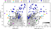 |
Fig. 7 Final masses of our simulated clusters, along with the simulated cluster from Vergara et al. (2025), are shown as star symbols. The current masses of YSCs from Brown & Gnedin (2021) are also included, with the color bar indicating their ages. Recent JWST observations of YMCs (Vanzella et al. 2022a,b, 2023; Mowla et al. 2024; Adamo et al. 2024) are shown with blue symbols, all plotted against the effective radius (left) and surface density (right). |
4 Summary and conclusions
We present simulations of the densest stellar clusters to date using NBODY6++GPU and the MOCCA code. Our models include the latest updates for stellar radius evolution and close encounter prescriptions (see Vergara et al. 2025). We have also updated the stellar rejuvenation treatment to ensure that when a VMS collides with a less massive star, its age does not change dramatically (see Appendix A for details). Wind prescriptions follow Vink et al. (2001), Vink & de Koter (2002), Vink & de Koter (2005), and Belczynski et al. (2010), with the helium-burning phases modeled using luminosity-dependent winds (Sander et al. 2020).
Our models represent stellar clusters with high density, and show BH seed formation through the purely collisional channel in a short period of time. Clusters with a higher initial number of stars experience more collisions, which can lead to the formation of more massive objects (e.g., models R005N750k and R005N500k). However, clusters with higher densities form massive objects more quickly (e.g., models R0005N50k and R001N250k). Clusters with more particles but lower densities undergo delayed core collapse and contain a larger reservoir of relatively massive stars that can migrate inward due to mass segregation. This results in more collisions over longer timescales, allowing the VMS to be repeatedly rejuvenated through mergers and postponing its collapse into a BH seed. In contrast, high-density clusters with fewer particles experience faster core collapse, triggering earlier collisions and rapid VMS growth. The VMS in these systems quickly increases its cross-section, further enhancing the collision rate. However, the stellar reservoir is depleted sooner, leading to the earlier collapse of the VMS into a BH seed. Overall, our results show that the formation and evolution of VMSs (and their subsequent collapse into BH seeds) depend on both the cluster’s density and its number of stars. Higher densities accelerate VMS formation, while a larger number of stars increases the eventual VMS mass. The timing of BH seed formation is regulated by the number of collisions that rejuvenate the VMS, thus, clusters with more stars form BH seeds later. Recent studies also indicate that mass loss in VMSs is highly sensitive to both the mass distribution of the colliding stars and the structural evolution of the VMS itself (Ramírez-Galeano et al. 2025).
Dense stellar clusters form in environments with low metallicity and high gas density (Fukushima & Yajima 2023), where radiative pressure is insufficient to prevent collapse. This leads to an extremely high SFE of around 80% (Menon et al. 2023; Somerville et al. 2025). Mergers of gas-rich dwarf galaxies at high redshift have also been proposed as a viable pathway for assembling massive, compact stellar systems (Renaud et al. 2015; Lahén et al. 2020a,b, 2025). Recent simulations suggest that, in such environments, the merger of star clusters hosting massive BHs can lead to the rapid formation of hard binary BH systems. These binaries interact strongly with surrounding stars and stellar-mass BHs, driving substantial ejection of both stellar and compact objects (Souvaitzis et al. 2025). Repeated ejections during and after cluster mergers can significantly reduce the final mass of the resulting cluster. These extremely dense stellar clusters are also ideal sites for the formation of supermassive stars through runaway collisions within their cores (Charbonnel et al. 2023).
Our models exhibit stellar collision rates much higher than those typically found in globular cluster simulations, such as the DRAGON-II runs (Arca Sedda et al. 2023, 2024b,a). In our simulations, the timescale for collisions is shorter than the thermal timescale of the VMS, preventing the star from reaching thermal equilibrium. This can drive radial expansion, increase the star’s cross-section, and further enhance the collision rate. In addition, this process rejuvenates the VMS, delaying the formation of a BH seed. The thermodynamic state of such a VMS remains poorly understood. Mass loss could be driven by stellar winds or by stellar mergers (Dale & Davies 2006), which also provide an additional enrichment pathway by ejecting processed material into the interstellar medium (Gieles et al. 2018; Wang et al. 2020). However, the assumed rapid thermal recovery after each collision allows mass growth to outpace wind-driven mass loss.
Very massive star formation through runaway stellar collisions in dense star clusters was first proposed analytically by Begelman & Rees (1978), Rees (1984), and Lee (1987). Subsequent studies employed Fokker–Planck and Monte Carlo methods (Quinlan & Shapiro 1990; Gürkan et al. 2004; Freitag et al. 2006a,b; Giersz et al. 2015) and direct N-body simulations (Vergara et al. 2023, 2025; Rantala & Naab 2025; Rantala et al. 2025). In this study, dense stellar systems allow us to explore their dynamics and their ability to form VMSs in a short time due to the constant bombardment of stars sinking toward the center. The deep gravitational potential presented in these stellar systems leads to the onset of collisions that quickly trigger the formation of a VMS ≳ 1000 M⊙ in less than 0.1 Myr.
For the YMCs observed with JWST, the collision-based formation scenario implies BH masses in the range of 102–105, M⊙ within these clusters. In our analysis, we considered both a conservative scenario (assuming the cluster masses and radii remain constant over time) and a more realistic scenario in which clusters undergo expansion, increasing the likelihood of forming massive objects due to higher initial densities. The numbers derived here are likely lower limits, as we did not account for the possible effects of gas. However, for more extended clusters, it is possible that massive object formation could be avoided in some cases. Moreover, the clusters observed with JWST are those that survived for a considerable period of time, while the densest clusters may have already collapsed and formed a massive BH at an earlier stage, as has been discussed by Escala (2021). The presence of these BHs could be confirmed or constrained with current and future X-ray observations. We also note that, while it is computationally challenging to model systems such as the observed little red dots (LRDs), their compactness naturally favors the collision-driven formation channel. It has been shown that the LRDs can have radii of 10 pc with core densities on the order of 108 M⊙ pc−3; note that this represents an upper and lower limit, respectively (Guia et al. 2024). It has been suggested that LRDs are favorable places for the formation of BH seeds (Pacucci et al. 2025; Escala et al. 2025; Taylor et al. 2025). Here we considered clusters with similar and higher central densities, but with smaller radii (and fewer particles), as otherwise, due to computational limitations, it is not feasible to explore these high densities.
TDEs, occurring when a star is torn apart by an IMBH’s tidal forces, produce luminous flares and provide insights into BH growth (Stone & Metzger 2016; Ryu et al. 2020b,c,a; Stone et al. 2020), which are particularly important for understanding LRD emissions (Bellovary 2025). Extreme mass ratio inspirals (EMRIs), in which stellar-mass BHs or neutron stars spiral into IMBHs via GW emission, are driven by dynamical friction and relativistic effects (Hils & Bender 1995; Broggi et al. 2022, 2024). Our models indicate rapid BH seed formation through runaway stellar collisions, suggesting that EMRIs could occur earlier in cosmic history than predicted. Multi-messenger astronomy enables testing these theories: TDE flares are observed by the Hubble Space Telescope (HST) (Leloudas et al. 2016) and Neil Gehrels Swift Observatory (Swift) (Brown et al. 2016), while GW detectors (LIGO/Virgo/KAGRA) (Abbott et al. 2024) and future missions ((LISA) (McCaffrey et al. 2025), and the Einstein Telescope (ET) (Punturo et al. 2010) target compact mergers and EMRIs.
Recent JWST observations of high-redshift galaxies have revealed unexpectedly high nitrogen abundances and elevated N/O ratios (Tacchella et al. 2023; Nagele & Umeda 2023; Maiolino et al. 2024; Larson et al. 2023; Marques-Chaves et al. 2024; Naidu et al. 2025; Ji et al. 2026, 2024; Isobe et al. 2025), a phenomenon that standard chemical evolution models struggle to explain (Cameron et al. 2023). While typical models predict low N/O ratios in young, low-metallicity systems (since nitrogen production is dominated by massive stars on longer timescales) the presence of VMSs offers a compelling solution. Very massive stars can rapidly enrich the interstellar medium with nitrogen through their strong winds and unique nucleosynthetic pathways, producing the high N/O ratios observed even in the early Universe (Charbonnel et al. 2023). Incorporating VMSs into chemical evolution models allows both the amount and timing of nitrogen enrichment to better match observations, making them a key factor in understanding the chemical signatures of young, high-redshift stellar populations.
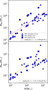 |
Fig. 8 Expected BH masses within YMCs against their current stellar mass. The top panel shows the conservative case, while the bottom panel shows the optimistic one. |
Data availability
The underlying data, including the initial model used in this work, as well as the output and diagnostic files from both the NBODY6++GPU and MOCCA simulations, are publicly available in the zenodo repository.
Acknowledgements
We thank the referees for their constructive comments and helpful suggestions, which improved the clarity and readability of the manuscript. M.C.V. acknowledges funding through ANID (Doctorado acuerdo bilateral DAAD/62210038) and DAAD (funding program number 57600326). M.C.V. acknowledges the International Max Planck Research School for Astronomy and Cosmic Physics at the University of Heidelberg (IMPRS-HD). A.A. acknowledges support for this paper from project No. 2021/43/P/ST9/03167 co-funded by the Polish National Science Center (NCN) and the European Union Framework Programme for Research and Innovation Horizon 2020 under the Marie Skłodowska-Curie grant agreement No. 945339. R.S. acknowledges NAOC International Cooperation Office for its support in 2023, 2024, and 2025, and the support by the National Science Foundation of China (NSFC) under grant No. 12473017. This research was supported in part by grant NSF PHY-2309135 to the Kavli Institute for Theoretical Physics (KITP). This material is based upon work supported by Tamkeen under the NYU Abu Dhabi Research Institute grant CASS. F.F.D. and R.S. acknowledge support by the German Science Foundation (DFG, project Sp 345/24-1). M.A.S. acknowledges funding from the European Union’s Horizon 2020 research and innovation programme under the Marie Skłodowska-Curie grant agreement No. 101025436 (project GRACE-BH, PI: Manuel Arca Sedda). M.A.S. acknowledge financial support from the MERAC foundation. D.R.G.S. gratefully acknowledges support by the ANID BASAL project FB21003 and ANID QUIMAL220002. D.R.G.S. thanks for funding via the Alexander von Humboldt – Foundation, Bonn, Germany. A.E. acknowledges financial support from the Center for Astrophysics and Associated Technologies CATA (FB210003). M.G. was supported by the Polish National Science Center (NCN) through the grant 2021/41/B/ST9/01191. Computations were performed on the HPC system Raven at the Max Planck Computing and Data Facility, and we also acknowledge the Gauss Centre for Supercomputing e.V. for computing time through the John von Neumann Institute for Computing (NIC) on the GCS Supercomputer JUWELS Booster at Jülich Supercomputing Centre (JSC). We also acknowledge A. Sander and his team for helpful comments.
References
- Aarseth, S. J. 1999, PASP, 111, 1333 [NASA ADS] [CrossRef] [Google Scholar]
- Abbott, R., Abe, H., Acernese, F., et al. 2024, ApJ, 966, 137 [Google Scholar]
- Adamo, A., Usher, C., Pfeffer, J., & Claeyssens, A. 2023, MNRAS, 525, L6 [NASA ADS] [CrossRef] [Google Scholar]
- Adamo, A., Bradley, L. D., Vanzella, E., et al. 2024, Nature, 632, 513 [NASA ADS] [CrossRef] [Google Scholar]
- Afanasiev, A. V., Chilingarian, I. V., Mieske, S., et al. 2018, MNRAS, 477, 4856 [Google Scholar]
- Ahmad, A., & Cohen, L. 1973, J. Comput. Phys., 12, 389 [Google Scholar]
- Alister Seguel, P. J., Schleicher, D. R. G., Boekholt, T. C. N., Fellhauer, M., & Klessen, R. S. 2020, MNRAS, 493, 2352 [NASA ADS] [CrossRef] [Google Scholar]
- Arca Sedda, M., Mapelli, M., Benacquista, M., & Spera, M. 2023, MNRAS, 520, 5259 [NASA ADS] [CrossRef] [Google Scholar]
- Arca Sedda, M., Kamlah, A. W. H., Spurzem, R., et al. 2024a, MNRAS, 528, 5119 [NASA ADS] [CrossRef] [Google Scholar]
- Arca Sedda, M., Kamlah, A. W. H., Spurzem, R., et al. 2024b, MNRAS, 528, 5140 [CrossRef] [Google Scholar]
- Askar, A., Szkudlarek, M., Gondek-Rosińska, D., Giersz, M., & Bulik, T. 2017, MNRAS, 464, L36 [CrossRef] [Google Scholar]
- Bamber, J., Shapiro, S. L., Ruiz, M., & Tsokaros, A. 2025, Phys. Rev. D, 112, 024046 [Google Scholar]
- Banerjee, S. 2021, MNRAS, 500, 3002 [Google Scholar]
- Banerjee, S., Belczynski, K., Fryer, C. L., et al. 2020, A&A, 639, A41 [NASA ADS] [CrossRef] [EDP Sciences] [Google Scholar]
- Begelman, M. C. 2010, MNRAS, 402, 673 [NASA ADS] [CrossRef] [Google Scholar]
- Begelman, M. C., & Rees, M. J. 1978, MNRAS, 185, 847 [NASA ADS] [CrossRef] [Google Scholar]
- Begelman, M. C., Volonteri, M., & Rees, M. J. 2006, MNRAS, 370, 289 [NASA ADS] [CrossRef] [Google Scholar]
- Belczynski, K., Bulik, T., Fryer, C. L., et al. 2010, ApJ, 714, 1217 [NASA ADS] [CrossRef] [Google Scholar]
- Bellovary, J. 2025, ApJ, 984, L55 [Google Scholar]
- Binney, J., & Tremaine, S. 2008, Galactic Dynamics, 2nd edn. (Princeton: Princeton University Press) [Google Scholar]
- Bond, J. R., Arnett, W. D., & Carr, B. J. 1984, ApJ, 280, 825 [NASA ADS] [CrossRef] [Google Scholar]
- Bouwens, R. J., Illingworth, G. D., González, V., et al. 2010, ApJ, 725, 1587 [NASA ADS] [CrossRef] [Google Scholar]
- Broggi, L., Bortolas, E., Bonetti, M., Sesana, A., & Dotti, M. 2022, MNRAS, 514, 3270 [NASA ADS] [CrossRef] [Google Scholar]
- Broggi, L., Stone, N. C., Ryu, T., et al. 2024, Open J. Astrophys., 7, 48 [CrossRef] [Google Scholar]
- Brown, G., & Gnedin, O. Y. 2021, MNRAS, 508, 5935 [NASA ADS] [CrossRef] [Google Scholar]
- Brown, P. J., Yang, Y., Cooke, J., et al. 2016, ApJ, 828, 3 [NASA ADS] [CrossRef] [Google Scholar]
- Cameron, A. J., Katz, H., Rey, M. P., & Saxena, A. 2023, MNRAS, 523, 3516 [NASA ADS] [CrossRef] [Google Scholar]
- Charbonnel, C., Schaerer, D., Prantzos, N., et al. 2023, A&A, 673, L7 [NASA ADS] [CrossRef] [EDP Sciences] [Google Scholar]
- Chon, S., & Omukai, K. 2025, MNRAS, 539, 2561 [Google Scholar]
- Dale, J. E., & Davies, M. B. 2006, MNRAS, 366, 1424 [NASA ADS] [Google Scholar]
- Di Carlo, U. N., Mapelli, M., Bouffanais, Y., et al. 2020, MNRAS, 497, 1043 [NASA ADS] [CrossRef] [Google Scholar]
- Escala, A. 2021, ApJ, 908, 57 [NASA ADS] [CrossRef] [Google Scholar]
- Escala, A., Zimmermann, L., Valdebenito, S., et al. 2025, ApJ, 995, 44 [Google Scholar]
- Fregeau, J. M., Cheung, P., Portegies Zwart, S. F., & Rasio, F. A. 2004, MNRAS, 352, 1 [CrossRef] [Google Scholar]
- Freitag, M., Gürkan, M. A., & Rasio, F. A. 2006a, MNRAS, 368, 141 [NASA ADS] [Google Scholar]
- Freitag, M., Rasio, F. A., & Baumgardt, H. 2006b, MNRAS, 368, 121 [NASA ADS] [CrossRef] [Google Scholar]
- Fryer, C. L., Belczynski, K., Wiktorowicz, G., et al. 2012, ApJ, 749, 91 [Google Scholar]
- Fujii, M. S., & Portegies Zwart, S. 2013, MNRAS, 430, 1018 [NASA ADS] [CrossRef] [Google Scholar]
- Fujii, M. S., & Portegies Zwart, S. 2016, ApJ, 817, 4 [NASA ADS] [CrossRef] [Google Scholar]
- Fukushima, H., & Yajima, H. 2023, MNRAS, 524, 1422 [Google Scholar]
- Gaete, B., Schleicher, D. R. G., Lupi, A., et al. 2024, A&A, 690, A378 [NASA ADS] [CrossRef] [EDP Sciences] [Google Scholar]
- Georgiev, I. Y., Böker, T., Leigh, N., Lützgendorf, N., & Neumayer, N. 2016, MNRAS, 457, 2122 [Google Scholar]
- Gieles, M., Charbonnel, C., Krause, M. G. H., et al. 2018, MNRAS, 478, 2461 [Google Scholar]
- Gieles, M., Erkal, D., Antonini, F., Balbinot, E., & Peñarrubia, J. 2021, Nat. Astron., 5, 957 [NASA ADS] [CrossRef] [Google Scholar]
- Giersz, M. 2001, MNRAS, 324, 218 [NASA ADS] [CrossRef] [Google Scholar]
- Giersz, M., & Heggie, D. C. 1996, MNRAS, 279, 1037 [NASA ADS] [Google Scholar]
- Giersz, M., & Heggie, D. C. 1997, MNRAS, 286, 709 [Google Scholar]
- Giersz, M., Heggie, D. C., & Hurley, J. R. 2008, MNRAS, 388, 429 [Google Scholar]
- Giersz, M., Heggie, D. C., Hurley, J. R., & Hypki, A. 2013, MNRAS, 431, 2184 [NASA ADS] [CrossRef] [Google Scholar]
- Giersz, M., Leigh, N., Hypki, A., Lützgendorf, N., & Askar, A. 2015, MNRAS, 454, 3150 [Google Scholar]
- Giesers, B., Dreizler, S., Husser, T.-O., et al. 2018, MNRAS, 475, L15 [NASA ADS] [CrossRef] [Google Scholar]
- Glebbeek, E., Pols, O. R., & Hurley, J. R. 2008, A&A, 488, 1007 [NASA ADS] [CrossRef] [EDP Sciences] [Google Scholar]
- Grudić, M. Y., Hafen, Z., Rodriguez, C. L., et al. 2023, MNRAS, 519, 1366 [Google Scholar]
- Guia, C. A., Pacucci, F., & Kocevski, D. D. 2024, Res. Notes Am. Astron. Soc., 8, 207 [Google Scholar]
- Gürkan, M. A., Freitag, M., & Rasio, F. A. 2004, ApJ, 604, 632 [NASA ADS] [CrossRef] [Google Scholar]
- Häberle, M., Neumayer, N., Seth, A., et al. 2024, Nature, 631, 285 [CrossRef] [Google Scholar]
- Harris, W. E. 1996, AJ, 112, 1487 [Google Scholar]
- Heggie, D. C. 2014, MNRAS, 445, 3435 [NASA ADS] [CrossRef] [Google Scholar]
- Hénon, M. 1971, Ap&SS, 13, 284 [Google Scholar]
- Hils, D., & Bender, P. L. 1995, ApJ, 445, L7 [NASA ADS] [CrossRef] [Google Scholar]
- Hurley, J. R., Pols, O. R., & Tout, C. A. 2000, MNRAS, 315, 543 [Google Scholar]
- Hurley, J. R., Shara, M. M., & Tout, C. A. 2002, ASP Conf. Ser., 279, 115 [Google Scholar]
- Hurley, J. R., Pols, O. R., Aarseth, S. J., & Tout, C. A. 2005, MNRAS, 363, 293 [NASA ADS] [CrossRef] [Google Scholar]
- Hut, P., Makino, J., & McMillan, S. 1995, ApJ, 443, L93 [NASA ADS] [CrossRef] [Google Scholar]
- Hypki, A., & Giersz, M. 2013, MNRAS, 429, 1221 [NASA ADS] [CrossRef] [Google Scholar]
- Isobe, Y., Maiolino, R., D’Eugenio, F., et al. 2025, MNRAS, 541, L71 [Google Scholar]
- Ji, X., Ubler, H., Maiolino, R., et al. 2024, MNRAS, 535, 881 [NASA ADS] [CrossRef] [Google Scholar]
- Ji, X., Belokurov, V., Maiolino, R., et al. 2026, MNRAS, 545, staf2110 [Google Scholar]
- Kamlah, A. W. H., Leveque, A., Spurzem, R., et al. 2022a, MNRAS, 511, 4060 [NASA ADS] [CrossRef] [Google Scholar]
- Kamlah, A. W. H., Spurzem, R., Berczik, P., et al. 2022b, MNRAS, 516, 3266 [CrossRef] [Google Scholar]
- Katz, H., Sijacki, D., & Haehnelt, M. G. 2015, MNRAS, 451, 2352 [Google Scholar]
- King, I. R. 1966, AJ, 71, 64 [Google Scholar]
- King, I. R., Hedemann, Jr., E., Hodge, S. M., & White, R. E. 1968, AJ, 73, 456 [Google Scholar]
- Klessen, R. S., & Glover, S. C. O. 2016, Saas-Fee Advanced Course, 43, 85 [Google Scholar]
- Kremer, K., Ye, C. S., Rui, N. Z., et al. 2020, ApJS, 247, 48 [NASA ADS] [CrossRef] [Google Scholar]
- Kroupa, P. 2001, MNRAS, 322, 231 [NASA ADS] [CrossRef] [Google Scholar]
- Kroupa, P., Subr, L., Jerabkova, T., & Wang, L. 2020, MNRAS, 498, 5652 [Google Scholar]
- Lahén, N., Naab, T., Johansson, P. H., et al. 2020a, ApJ, 904, 71 [CrossRef] [Google Scholar]
- Lahén, N., Naab, T., Johansson, P. H., et al. 2020b, ApJ, 891, 2 [CrossRef] [Google Scholar]
- Lahén, N., Naab, T., Rantala, A., & Partmann, C. 2025, MNRAS, 543, 1023 [Google Scholar]
- Larson, R. L., Finkelstein, S. L., Kocevski, D. D., et al. 2023, ApJ, 953, L29 [NASA ADS] [CrossRef] [Google Scholar]
- Lee, H. M. 1987, ApJ, 319, 801 [CrossRef] [Google Scholar]
- Leloudas, G., Fraser, M., Stone, N. C., et al. 2016, Nat. Astron., 1, 0002 [Google Scholar]
- Liempi, M., Schleicher, D. R. G., Benson, A., Escala, A., & Vergara, M. C. 2025, A&A, 694, A42 [NASA ADS] [CrossRef] [EDP Sciences] [Google Scholar]
- Linden, S. T., Lai, T., Evans, A. S., et al. 2024, ApJ, 974, L27 [Google Scholar]
- Liu, S., Wang, L., Hu, Y.-M., Tanikawa, A., & Trani, A. A. 2024, MNRAS, 533, 2262 [NASA ADS] [CrossRef] [Google Scholar]
- Lodato, G., & Natarajan, P. 2006, MNRAS, 371, 1813 [NASA ADS] [CrossRef] [Google Scholar]
- Loeb, A., & Rasio, F. A. 1994, ApJ, 432, 52 [Google Scholar]
- Longmore, S. N., Kruijssen, J. M. D., Bastian, N., et al. 2014, in Protostars and Planets VI, eds. H. Beuther, R. S. Klessen, C. P. Dullemond, & T. Henning (Tucson: University of Arizona Press), 291 [Google Scholar]
- Longmore, S. N., Chevance, M., & Kruijssen, J. M. D. 2021, ApJ, 911, L16 [NASA ADS] [CrossRef] [Google Scholar]
- Lupi, A., Colpi, M., Devecchi, B., Galanti, G., & Volonteri, M. 2014, MNRAS, 442, 3616 [NASA ADS] [CrossRef] [Google Scholar]
- Lützgendorf, N., Kissler-Patig, M., Neumayer, N., et al. 2013, A&A, 555, A26 [NASA ADS] [CrossRef] [EDP Sciences] [Google Scholar]
- Madau, P., & Rees, M. J. 2001, ApJ, 551, L27 [Google Scholar]
- Madrid, J. P., Leigh, N. W. C., Hurley, J. R., & Giersz, M. 2017, MNRAS, 470, 1729 [NASA ADS] [CrossRef] [Google Scholar]
- Maiolino, R., Scholtz, J., Witstok, J., et al. 2024, Nature, 627, 59 [NASA ADS] [CrossRef] [Google Scholar]
- Makino, J. 1999, J. Comput. Phys., 151, 910 [Google Scholar]
- Makino, J., & Aarseth, S. J. 1992, PASJ, 44, 141 [NASA ADS] [Google Scholar]
- Maliszewski, K., Giersz, M., Gondek-Rosinska, D., Askar, A., & Hypki, A. 2022, MNRAS, 514, 5879 [NASA ADS] [CrossRef] [Google Scholar]
- Mapelli, M. 2016, MNRAS, 459, 3432 [NASA ADS] [CrossRef] [Google Scholar]
- Marques-Chaves, R., Schaerer, D., Kuruvanthodi, A., et al. 2024, A&A, 681, A30 [NASA ADS] [CrossRef] [EDP Sciences] [Google Scholar]
- McCaffrey, J., Regan, J., Smith, B., et al. 2025, Open J. Astrophys., 8, 11 [Google Scholar]
- Menon, S. H., Federrath, C., & Krumholz, M. R. 2023, MNRAS, 521, 5160 [NASA ADS] [CrossRef] [Google Scholar]
- Messa, M., Vanzella, E., Loiacono, F., et al. 2026, A&A, 705, A173 [NASA ADS] [CrossRef] [EDP Sciences] [Google Scholar]
- Mestichelli, B., Mapelli, M., Torniamenti, S., et al. 2024, A&A, 690, A106 [NASA ADS] [CrossRef] [EDP Sciences] [Google Scholar]
- Mikkola, S., & Aarseth, S. J. 1989, Celest. Mech. Dyn. Astron., 47, 375 [Google Scholar]
- Mikkola, S., & Aarseth, S. J. 1993, Celest. Mech. Dyn. Astron., 57, 439 [NASA ADS] [CrossRef] [Google Scholar]
- Miller, M. C., & Davies, M. B. 2012, ApJ, 755, 81 [NASA ADS] [CrossRef] [Google Scholar]
- Mowla, L., Iyer, K., Asada, Y., et al. 2024, Nature, 636, 332 [Google Scholar]
- Nagele, C., & Umeda, H. 2023, ApJ, 949, L16 [NASA ADS] [CrossRef] [Google Scholar]
- Naidu, R. P., Oesch, P. A., Brammer, G., et al. 2025, arXiv e-prints [arXiv:2505.11263] [Google Scholar]
- Nandal, D., Sibony, Y., & Tsiatsiou, S. 2024, A&A, 688, A142 [NASA ADS] [CrossRef] [EDP Sciences] [Google Scholar]
- Neumayer, N., Seth, A., & Böker, T. 2020, A&A Rev., 28, 4 [NASA ADS] [CrossRef] [Google Scholar]
- Omukai, K., & Nishi, R. 1998, ApJ, 508, 141 [NASA ADS] [CrossRef] [Google Scholar]
- Pacucci, F., Hernquist, L., & Fujii, M. 2025, ApJ, 994, 40 [Google Scholar]
- Panamarev, T., Just, A., Spurzem, R., et al. 2019, MNRAS, 484, 3279 [NASA ADS] [CrossRef] [Google Scholar]
- Plummer, H. C. 1911, MNRAS, 71, 460 [Google Scholar]
- Polak, B., Mac Low, M.-M., Klessen, R. S., et al. 2024, A&A, 690, A94 [NASA ADS] [CrossRef] [EDP Sciences] [Google Scholar]
- Portegies Zwart, S. F., & McMillan, S. L. W. 2002, ApJ, 576, 899 [Google Scholar]
- Portegies Zwart, S. F., Makino, J., McMillan, S. L. W., & Hut, P. 1999, A&A, 348, 117 [NASA ADS] [Google Scholar]
- Portegies Zwart, S. F., Baumgardt, H., Hut, P., Makino, J., & McMillan, S. L. W. 2004, Nature, 428, 724 [Google Scholar]
- Punturo, M., Abernathy, M., Acernese, F., et al. 2010, Class. Quantum Gravity, 27, 194002 [NASA ADS] [CrossRef] [Google Scholar]
- Quinlan, G. D., & Shapiro, S. L. 1990, ApJ, 356, 483 [NASA ADS] [CrossRef] [Google Scholar]
- Ramírez-Galeano, L., Charbonnel, C., Fragos, T., et al. 2025, A&A, 699, A223 [NASA ADS] [CrossRef] [EDP Sciences] [Google Scholar]
- Rantala, A., & Naab, T. 2025, MNRAS, 542, L78 [Google Scholar]
- Rantala, A., Naab, T., Rizzuto, F. P., et al. 2023, MNRAS, 522, 5180 [CrossRef] [Google Scholar]
- Rantala, A., Lahén, N., Naab, T., Escobar, G. J., & Iorio, G. 2025, MNRAS, 543, 2130 [Google Scholar]
- Rastello, S., Mapelli, M., Di Carlo, U. N., et al. 2021, MNRAS, 507, 3612 [CrossRef] [Google Scholar]
- Rees, M. J. 1978, The Observatory, 98, 210 [NASA ADS] [Google Scholar]
- Rees, M. J. 1984, ARA&A, 22, 471 [Google Scholar]
- Reinoso, B., Schleicher, D. R. G., Fellhauer, M., Klessen, R. S., & Boekholt, T. C. N. 2018, A&A, 614, A14 [NASA ADS] [CrossRef] [EDP Sciences] [Google Scholar]
- Reinoso, B., Schleicher, D. R. G., Fellhauer, M., Leigh, N. W. C., & Klessen, R. S. 2020, A&A, 639, A92 [NASA ADS] [CrossRef] [EDP Sciences] [Google Scholar]
- Reinoso, B., Latif, M. A., & Schleicher, D. R. G. 2025, A&A, 700, A66 [NASA ADS] [CrossRef] [EDP Sciences] [Google Scholar]
- Renaud, F., Bournaud, F., & Duc, P.-A. 2015, MNRAS, 446, 2038 [Google Scholar]
- Ricarte, A., & Natarajan, P. 2018, MNRAS, 481, 3278 [NASA ADS] [CrossRef] [Google Scholar]
- Rizzuto, F. P., Naab, T., Spurzem, R., et al. 2021, MNRAS, 501, 5257 [NASA ADS] [CrossRef] [Google Scholar]
- Rizzuto, F. P., Naab, T., Rantala, A., et al. 2023, MNRAS, 521, 2930 [NASA ADS] [CrossRef] [Google Scholar]
- Rodriguez, C. L., Zevin, M., Amaro-Seoane, P., et al. 2019, Phys. Rev. D, 100, 043027 [Google Scholar]
- Rodriguez, C. L., Weatherford, N. C., Coughlin, S. C., et al. 2022, ApJS, 258, 22 [NASA ADS] [CrossRef] [Google Scholar]
- Ryu, T., Krolik, J., Piran, T., & Noble, S. C. 2020a, ApJ, 904, 99 [NASA ADS] [CrossRef] [Google Scholar]
- Ryu, T., Krolik, J., Piran, T., & Noble, S. C. 2020b, ApJ, 904, 100 [NASA ADS] [CrossRef] [Google Scholar]
- Ryu, T., Krolik, J., Piran, T., & Noble, S. C. 2020c, ApJ, 904, 101 [NASA ADS] [CrossRef] [Google Scholar]
- Sakurai, Y., Yoshida, N., Fujii, M. S., & Hirano, S. 2017, MNRAS, 472, 1677 [NASA ADS] [CrossRef] [Google Scholar]
- Salpeter, E. E. 1955, ApJ, 121, 161 [Google Scholar]
- Sander, A. A. C., Vink, J. S., & Hamann, W.-R. 2020, MNRAS, 491, 4406 [Google Scholar]
- Sanders, R. H. 1970, ApJ, 162, 791 [Google Scholar]
- Scalo, J. M. 1986, FCP, 11, 1 [Google Scholar]
- Shapiro, S. L., & Teukolsky, S. A. 1985, ApJ, 292, L41 [NASA ADS] [CrossRef] [Google Scholar]
- Solar, P. A., Reinoso, B., Schleicher, D. R. G., Klessen, R. S., & Banerjee, R. 2025, A&A, 699, A64 [NASA ADS] [CrossRef] [EDP Sciences] [Google Scholar]
- Somerville, R. S., Yung, L. Y. A., Lancaster, L., et al. 2025, MNRAS, 544, 3774 [Google Scholar]
- Souvaitzis, L., Rantala, A., & Naab, T. 2025, MNRAS, 539, 45 [Google Scholar]
- Spitzer, Jr., L., & Saslaw, W. C. 1966, ApJ, 143, 400 [NASA ADS] [Google Scholar]
- Spitzer, Jr., L., & Stone, M. E. 1967, ApJ, 147, 519 [Google Scholar]
- Spurzem, R. 1999, J. Comput. Appl. Math., 109, 407 [CrossRef] [Google Scholar]
- Spurzem, R., & Kamlah, A. 2023, Liv. Rev. Comput. Astrophys., 9, 3 [CrossRef] [Google Scholar]
- Stiefel, E., & Kustaanheimo, P. 1965, Journal für die reine und angewandte Mathematik, 218, 204 [Google Scholar]
- Stodolkiewicz, J. S. 1982, Acta Astron., 32, 63 [NASA ADS] [Google Scholar]
- Stodolkiewicz, J. S. 1986, Acta Astron., 36, 19 [NASA ADS] [Google Scholar]
- Stone, N. C., & Metzger, B. D. 2016, MNRAS, 455, 859 [NASA ADS] [CrossRef] [Google Scholar]
- Stone, N. C., Küpper, A. H. W., & Ostriker, J. P. 2017, MNRAS, 467, 4180 [NASA ADS] [Google Scholar]
- Stone, N. C., Vasiliev, E., Kesden, M., et al. 2020, Space Sci. Rev., 216, 35 [NASA ADS] [CrossRef] [Google Scholar]
- Tacchella, S., Eisenstein, D. J., Hainline, K., et al. 2023, ApJ, 952, 74 [NASA ADS] [CrossRef] [Google Scholar]
- Tan, J. C., & McKee, C. F. 2004, ApJ, 603, 383 [CrossRef] [Google Scholar]
- Taylor, A. J., Kokorev, V., Kocevski, D. D., et al. 2025, ApJ, 989, L7 [Google Scholar]
- Tsiatsiou, S., Sibony, Y., Nandal, D., et al. 2024, A&A, 687, A307 [NASA ADS] [CrossRef] [EDP Sciences] [Google Scholar]
- Vanzella, E., Castellano, M., Bergamini, P., et al. 2022a, A&A, 659, A2 [NASA ADS] [CrossRef] [EDP Sciences] [Google Scholar]
- Vanzella, E., Castellano, M., Bergamini, P., et al. 2022b, ApJ, 940, L53 [NASA ADS] [CrossRef] [Google Scholar]
- Vanzella, E., Claeyssens, A., Welch, B., et al. 2023, ApJ, 945, 53 [NASA ADS] [CrossRef] [Google Scholar]
- Vanzella, E., Messa, M., Adamo, A., et al. 2026, A&A, 705, A171 [NASA ADS] [CrossRef] [EDP Sciences] [Google Scholar]
- Vergara, M. Z. C., Schleicher, D. R. G., Boekholt, T. C. N., et al. 2021, A&A, 649, A160 [NASA ADS] [CrossRef] [EDP Sciences] [Google Scholar]
- Vergara, M. C., Escala, A., Schleicher, D. R. G., & Reinoso, B. 2023, MNRAS, 522, 4224 [NASA ADS] [CrossRef] [Google Scholar]
- Vergara, M. C., Schleicher, D. R. G., Escala, A., et al. 2024, A&A, 689, A34 [NASA ADS] [CrossRef] [EDP Sciences] [Google Scholar]
- Vergara, M. C., Askar, A., Kamlah, A. W. H., et al. 2025, A&A, 704, A321 [NASA ADS] [CrossRef] [EDP Sciences] [Google Scholar]
- Vink, J. S. 2018, A&A, 615, A119 [NASA ADS] [CrossRef] [EDP Sciences] [Google Scholar]
- Vink, J. S., & de Koter, A. 2002, A&A, 393, 543 [NASA ADS] [CrossRef] [EDP Sciences] [Google Scholar]
- Vink, J. S., & de Koter, A. 2005, A&A, 442, 587 [NASA ADS] [CrossRef] [EDP Sciences] [Google Scholar]
- Vink, J. S., de Koter, A., & Lamers, H. J. G. L. M. 2001, A&A, 369, 574 [NASA ADS] [CrossRef] [EDP Sciences] [Google Scholar]
- Voggel, K. T., Seth, A. C., Neumayer, N., et al. 2018, ApJ, 858, 20 [CrossRef] [Google Scholar]
- Volonteri, M., Haardt, F., & Madau, P. 2003, ApJ, 582, 559 [Google Scholar]
- Wang, L., Spurzem, R., Aarseth, S., et al. 2015, MNRAS, 450, 4070 [NASA ADS] [CrossRef] [Google Scholar]
- Wang, L., Spurzem, R., Aarseth, S., et al. 2016, MNRAS, 458, 1450 [Google Scholar]
- Wang, L., Kroupa, P., Takahashi, K., & Jerabkova, T. 2020, MNRAS, 491, 440 [Google Scholar]
- Wang, L., Fujii, M. S., & Tanikawa, A. 2021, MNRAS, 504, 5778 [NASA ADS] [CrossRef] [Google Scholar]
- Wang, L., Tanikawa, A., & Fujii, M. S. 2022, MNRAS, 509, 4713 [Google Scholar]
- Wang, L., Gieles, M., Baumgardt, H., et al. 2024, MNRAS, 527, 7495 [Google Scholar]
Monte Carlo Cluster simulAtor.
This relation holds for isolated clusters without mass loss (Giersz & Heggie 1996, 1997). For tidally limited clusters, post core-collapse expansion can still be approximated by a power law rh ∝ t(2–μ)/3, where the index μ depends on the rate of mass loss.
Appendix A Treatment of the rejuvenation of a star through collisions
The rejuvenation of a main-sequence star upon collisions with other main-sequence stars was numerically implemented by Hurley et al. (2002, 2005). The main motivation for the introduction was to provide a proper treatment of blue straggler stars. These stars consistently find themselves above a stellar populations MS turn-off point (see e.g., for observational evidence, check Giesers et al. 2018). This implies that the effective age, AMS, of these MS stars after a collision and a merger, is younger than the average age of the stellar population. In our models, which provide many collisions of a VMS with small mass MS stars, this treatment is not correct for the VMS, as the mass ratio q,
![Mathematical equation: $\[q=\frac{M_{\mathrm{MS}, 2}}{M_{\mathrm{MS}, 1}}\]$](/articles/aa/full_html/2026/03/aa56878-25/aa56878-25-eq4.png) (A.1)
(A.1)
becomes very small (i.e., q ≪ 1).
If we work under the base assumption that hydrogen in the MS core is uniformly distributed, then, after a collision, we have a convective mixing of the hydrogen fuel from envelope to core. The BSE code terminates the MS phase of the star and enters the Hertzsprung gap (HG) phase after 10 % of the total amount of hydrogen in the MS star has been burned (Hurley et al. 2000, 2005), the computational application is described below. We first consider the collision of two MS stars with (effective) ages AMS,1 and AMS,2, MS life-times τMS,1 and τMS,2, as well as masses MMS,1 and MMS,2, respectively. Here, the subscripts 1 and 2 denote the primary (and more massive) MS star and the secondary star, respectively. The collision produces the "third" MS star with effective age AMS,3, MS life time τMS,3 and mass MMS,3. If we know these parameters, (as suggested in Hurley et al. 2005) we can evaluate the final effective age AH,MS,3 of the produced MS star with their equation (see also Glebbeek et al. 2008, for more information).This treatment works well for MS collisions that have mass ratios q ≈ 1, which might be expected for many blue stragglers.
Here we have updated the traditional treatment, finding the age of the newly formed MS star as:
![Mathematical equation: $\[F_q=1.0-q \cdot(1.0-0.1 /(1+q)),\]$](/articles/aa/full_html/2026/03/aa56878-25/aa56878-25-eq5.png) (A.2)
(A.2)
![Mathematical equation: $\[A_{\mathrm{MS}, 3}=\tau_{M S, 3} \cdot F_q \cdot\left(A_{\mathrm{MS}, 1} / \tau_{M S, 1}-q \cdot A_{\mathrm{MS}, 2} / \tau_{M S, 2}\right).\]$](/articles/aa/full_html/2026/03/aa56878-25/aa56878-25-eq6.png) (A.3)
(A.3)
This treatment for the age of the VMS ensures that (i) if q → 1 and Fq → 1 (that is, the two colliding stars have similar masses), we get Eq. A.3, while (ii) for q → 0 and Fq → 0 (that is, the primary star is much more massive than the secondary star) the age of the VMS does not change significantly. This approach improves on the traditional treatment by ensuring a physically reasonable behavior in the limit q ≪ 1. In such cases, the secondary star contributes very little mass, and thus the merger product should retain an age close to that of the more massive primary. The introduction of the factor Fq ensures that the rejuvenation is suppressed when q is small, preventing an unrealistically young apparent age for the merger product. In contrast, earlier models lacking such a correction could significantly underestimate the age in this regime, resulting in overly rejuvenated stars even when the secondary’s contribution is negligible.
Appendix B Treatment of collisions in MOCCA
In the models with the shortest crossing and relaxation times considered in this work, specifically the R0005N50K, R001N100K, and R001N250K runs (see Fig. B.1), we found that the standard MOCCA collision treatment, based on local density and cross-section estimates, leads to unrealistically rapid growth of the VMS. In particular, before our improvements, the mass of the VMS would increase by more than a factor of two to three, compared to results from direct N-body simulations, indicating that collisions with VMS were overpredicted in these extreme regimes. To address this, we developed and implemented an improved, physically motivated treatment for VMS collisions in these high-density, low-N models. After introducing this new prescription, the MOCCA results for VMS growth were brought into good agreement with direct N-body simulations.
In standard MOCCA simulations, the probability for a collision between two single stars is computed using the cross-section formalism:
![Mathematical equation: $\[P_{\text {coll }}=0.5 ~C~ p_{\max }^2 ~n ~u ~\Delta t\]$](/articles/aa/full_html/2026/03/aa56878-25/aa56878-25-eq7.png) (B.1)
(B.1)
where C is a normalization constant, pmax is the maximum impact parameter (related to the sum of stellar radii and gravitational focusing), n is the local number density, u is the relative velocity, and Δt is the timestep. The collision outcome is then determined probabilistically, and, if a collision occurs, the two stars are merged.
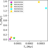 |
Fig. B.1 Initial half-mass relaxation time (Trx) versus initial crossing time (Tcr) for the five cluster models simulated in this work. The three models with the shortest relaxation and crossing times (R0005N50k, R001N100k, and R001N250k) required a modified collision treatment, since the standard local-density-based prescription significantly overestimates the collision rate in these extreme regimes |
For these compact models (Rh ≤ 0.01 pc) with relatively low number of stars, this cross-section-based approach becomes inaccurate because the presence of a VMS can dominate the local gravitational potential, invalidating the assumptions of the local density formalism and leading to overestimated collision rates. To address this limitation, we introduced a more physically motivated, two-body treatment for collisions involving VMSs, defined here as stars with M ≥ MVMS,th, where MVMS,th = 500 M⊙ in our production runs. This new approach assumes that, in the presence of a dominant central VMS, gravitational focusing and two-body orbital dynamics, rather than the local stellar density, govern whether a close passage results in a physical collision. In this approach, instead of applying the probabilistic cross-section formula, we explicitly compute the Keplerian orbital parameters for stars that are closest to each VMS in the system.
For each collision candidate pair where the primary star satisfies M1 ≥ MVMS,th, we compute the specific energy and specific angular momentum of the secondary star (hereafter, “star 2”) with respect to the VMS (“star 1”):
![Mathematical equation: $\[\epsilon_2=\frac{1}{2}\left(v_{r, 2}^2+v_{t, 2}^2\right)-\frac{G M_1}{r_2}\]$](/articles/aa/full_html/2026/03/aa56878-25/aa56878-25-eq8.png) (B.2)
(B.2)
![Mathematical equation: $\[\ell_2=r_2\left|v_{t, 2}\right|\]$](/articles/aa/full_html/2026/03/aa56878-25/aa56878-25-eq9.png) (B.3)
(B.3)
where vr,2 and vt,2 are the radial and tangential velocities of star 2 with respect to the VMS, r2 is its distance from the VMS, and G is the gravitational constant (set to unity in code units).
The pericenter distance of star 2 with respect to the VMS is then given by
![Mathematical equation: $\[r_{\mathrm{p}, 2}=\frac{-G M_1+\sqrt{\left(G M_1\right)^2+2 \epsilon_2 \ell_2^2}}{2 \epsilon_2}.\]$](/articles/aa/full_html/2026/03/aa56878-25/aa56878-25-eq10.png) (B.4)
(B.4)
If ϵ2 ≈ 0 (parabolic approach), we instead use
![Mathematical equation: $\[r_{\mathrm{p}, 2}=\frac{\ell_2^2}{2 G M_1}.\]$](/articles/aa/full_html/2026/03/aa56878-25/aa56878-25-eq11.png) (B.5)
(B.5)
A physical collision is deemed to occur if rp,2 ≤ R1 + R2, where R1 and R2 are the radii of the two stars. In this case, the collision is forced (Pcoll = 1), bypassing the original probabilistic cross-section calculation. If the pericenter is greater than the sum of the radii, no collision occurs.
The modified treatment is applied only when the more massive star in the pair exceeds the VMS mass threshold. For other star pairs, we use the original cross-section-based approach. For efficiency, and to mimic the high rate of encounters expected in extreme environments, this pericenter criterion is applied to a fixed number of the nearest neighbours of the VMS during each timestep. Specifically, we use the 30 nearest stars for the R0005N50k and R001N100k models, and 100 neighbours for the R001N250k run. All other aspects of the collision and merger handling, such as mass loss, rejuvenation, and product type, remain as in the standard MOCCA prescription.
We also applied this modified routine to the R005N500k model, where the pericenter test was used for the 200 nearest neighbours of each VMS. In that case, the combination of a larger neighbour set and a smaller timestep led to significantly improved agreement between MOCCA and direct N-body results for VMS growth. Without the new treatment, for the R00SN500k run, the standard collision prescription overestimated the IMBH mass at formation by about 5,000, M⊙ (25,000, M⊙ versus 20,000, M⊙ in the direct N-body simulation).
For the R0075N750k model, however, we found that the new prescription underpredicted the final IMBH mass relative to the direct N-body result. Therefore, for this highest-N case, we retained the original MOCCA collision treatment. As shown previously by Vergara et al. (2025), the agreement between MOCCA and direct N-body simulations is reasonable for large-N models when the standard probability-based collision treatment is used. In such high-N clusters, the larger number of massive stars provides a significant reservoir of potential collision partners for the VMS, enabling continuous growth over several Myr. Additionally, the longer relaxation time in these systems means that mass segregation and the subsequent delivery of massive stars to the cluster center proceeds more gradually, supporting a more extended phase of VMS growth.
In summary, we replaced the cross-section-based probabilistic collision criterion with a two-body pericenter test for VMSs, as described by the equations above. This suppresses artificially high collision rates in extreme-density, low-N runs and yields a more physical growth rate for VMSs, bringing the MOCCA results into agreement with the direct N-body simulations. We emphasize that this represents only a first step toward developing an improved and more general treatment for collisions involving a VMS or a central IMBH. In future work, we plan to implement and test more sophisticated prescriptions, guided by systematic comparisons with direct N-body simulations.
Appendix C Number of collisions and mass contribution
We analyze the number of stellar collisions and their mass contributions to VMS and BH seed formation, from both simulation codes.
Fig. C.1 presents histograms of the number of collisions across different mass ranges. The results from the N-body simulations are shown with solid bars, while those from the MOCCA code are indicated with hatched bars. The histogram bins correspond to the following mass intervals: < 0.1, 0.1–1, 1–10, 10–100, and > 100 M⊙. Each panel represents a different model from top to bottom: R0005N50k, R001N100k, R001N250k, R005N500k and R005N750k. The number of collisions for the different mass range in each models is listed below, the first set corresponds to the N-body, and the second to the MOCCA results:
Model R0005N50k:
N-body: 92, 762, 200, 76, 5
MOCCA: 54, 351, 193, 108, 75
Model R001N100k:
N-body: 139, 1046, 223, 156, 7
MOCCA: 12, 145, 96, 143, 8
Model R001N250k:
N-body: 571, 4156, 796, 404, 29
MOCCA: 71, 508, 268, 280, 55
Model R005N500k:
N-body: 491, 3503, 677, 383, 46
MOCCA: 342, 2357, 494, 358, 45
Model R005N750k:
N-body: 1072, 7649, 1442, 685, 71
MOCCA: 271, 2176, 1124, 767, 79
Fig. C.2 presents histograms of the mass contribution to the VMS and BH seed formation. The bar styles, panels, bin mass intervals, and bullet points are the same as in Fig. C.1, the results are:
Model R0005N50k:
N-body: 8.20, 265.42, 722.30, 2237.57, 709.96 M⊙
MOCCA: 4.74, 125.72, 715.84, 2921.03, 842.85 M⊙
Model R001N100k:
N-body: 12.41, 336.44, 682.50, 5082.01, 920.88 M⊙
MOCCA: 1.09, 53.68, 396.52, 5344.29, 1055.53 M⊙
Model R001N250k:
N-body: 50.99, 1377.53, 2355.33, 12805.41, 4039.95 M⊙
MOCCA: 6.32, 180.35, 1042.07, 10343.75, 8502.78 M⊙
Model R005N500k:
N-body: 43.77, 1146.33, 2067.01, 14622.21, 5835.47 M⊙
MOCCA: 30.56, 789.12, 1671.15, 13943.06, 5420.96 M⊙
Model R005N750k:
N-body: 95.80, 2490.73, 4241.25, 24527.13, 9636.05 M⊙
MOCCA: 24.21, 754.99, 4565.79, 22993.53, 12946.69 M⊙
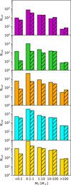 |
Fig. C.1 Histograms showing the number of collisions contributing to VMS and BH seed formation. The mass bins are: < 0.1 M⊙, 0.1–1 M⊙, 1–10 M⊙, 10–100 M⊙, and > 100 M⊙. Results are shown for both the N-body simulations (solid bars) and the MOCCA simulations (hatched bars). From top to bottom, the models are R0005N50k, R001N100k, R001N250k, R005N500k, and R005N750k. |
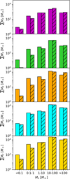 |
Fig. C.2 Histograms showing the cumulative mass contributed to VMS and BH seed formation. The mass bins and bar styles are the same as in Fig. C.1. |
Both codes produce different numbers of collisions within the mass interval bins, resulting in varying mass contributions, despite starting from the same initial conditions. The models R0005N50k, R001N100k, R001N250k, R005N500k, and R00SN750k initially contain 5, 5, 30, 57, and 79 stars with masses > 100 M⊙, respectively. However, in the MOCCA simulations, the VMS shows a greater contribution from stars with masses > 100 M⊙ in the R0005N50k, R001N100k, and R001N250k models. This occurs because the standard MOCCA prescription forms massive stars earlier, which then sink and collide with the VMS. The high densities presented in these clusters, quickly form a VMS in the center that bound several low-mass stars. The new collision treatment implemented in MOCCA, implies that if a star presents a pericenter distance slightly greater than the sum of the radii of its two stars, it is not considered as a candidate to collide with the VMS, however, due to the standard collision treatment, they will be candidates to collide with other stars that present similar conditions (i.e. rp,2 > R1 + R2), thus implying that they might collide with each other, forming a more massive star, that later sink to the center. This extremely dense regime for the star cluster challenges the standard collision treatment in MOCCA, this new update is the first attempt to treat collisions in the proximity of a single massive object at the center, however, the general agreement on the final outcome of both codes is a very good sign that we are on the right track, in the future we will further improve the treatment in MOCCA to obtain better overall agreement for the number of collisions we see with direct N-body.
Appendix D Number of escapers and type of direct collisions in N-body
We analyze the number of escapers, binary and hyperbolic collisions across our models. This analysis is limited to N-body simulations. In MOCCA, all recorded collisions are treated as hyperbolic encounters, since the code does not explicitly follow the orbital motion of stars, thus is not possible to distinguish between binary and hyperbolic collisions.
In Fig. D.1, models R0005N50k, R001N100k, and R001N250k present hyperbolic collisions within the first 100 yr, while binary collisions appear later around 1000 yr. Notably, the appearance of escaping stars coincides with the onset of binary collisions. Model R005N500k, both hyperbolic and binary collisions occur almost simultaneously at early times. However, hyperbolic encounters dominate for the first few thousand years. Still, the number of escapers begins to rise significantly once the rate of binary collisions increases. Model R005N750k, also shows early hyperbolic collisions, with a single escape occurring prior to any binary collisions. Nevertheless, a notable increase in escapers follows the onset of binary encounters.
In general, we observe that hyperbolic collisions generally occur earlier than binary collisions. The number of escaping stars begins to increase notably as the number of binary collisions rises. This suggests that the stellar escapes are primarily driven by binary interactions.
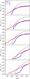 |
Fig. D.1 Time evolution of the number of escaping stars (dashed black line) and the number of binary (solid blue line) and hyperbolic (solid red line) collisions. From top to bottom, the models are R0005N50k, R001N100k, R001N250k, R005N500k, and R005N750k. |
All Tables
All Figures
|
Fig. 1 Initial half-mass density ρh, computed at the initial half-mass radius rh, is expressed as a function of the initial number of stars N. The figure has been reproduced from Arca Sedda et al. (2023, 2024b,a) and adapted to include a color bar with the logarithm of the average half-mass radius. We include other simulations and the new ones presented in this paper. |
| In the text | |
|
Fig. 2 Initial and final masses and half-mass radii of the clusters. The dotted lines represent when the timescales (tcoll and trx) are equal to τ = 4 Myr. The shaded regions indicate the parameter space where the respective timescales fall within the range 1 Myr ≤ τ ≤ 10 Gyr, highlighting different dynamical regimes: pink for two-body relaxation and gray for stellar collisions. Our clusters R0005N50k, R001N100k, R001N250k, R005N500k, and R005N750k evolve for 3.73, 3.81, 3.64, 3.80, and 3.87 Myr, respectively. We show their initial conditions with empty symbols and the final conditions with filled symbols, connected by arrows. |
| In the text | |
|
Fig. 3 Lagrangian radii calculated from the initial mass of the cluster for the 90, 70, 50, 30, 10, and 1% of the enclosed mass of model R005N750k (top) and model R0005N50k (bottom). |
| In the text | |
|
Fig. 4 Time evolution of the cumulative escaping mass normalized by the initial cluster mass (top) and the number of collisions with the most massive object normalized by the initial particle numbers (bottom). The solid lines are for N-body simulations and the dashed lines are for MOCCA ones. |
| In the text | |
|
Fig. 5 Time evolution of the mass growth of VMSs that collapse into BH seeds. Solid lines represent N-body simulations and dashed lines MOCCA ones. |
| In the text | |
|
Fig. 6 BH formation efficiency as a function of the ratio of initial cluster mass to critical mass. The figure has been reproduced from Vergara et al. (2024); we fit an asymmetric sigmoid function, represented by the dashed black line. The shaded gray bands represent the confidence intervals estimated by bootstrap resampling: the darker, middle, and lighter gray bands correspond to the 1σ, 2σ, and 3σ uncertainty regions. These intervals quantify the uncertainty in the fit curve, arising from data variability. We added the simulation from Vergara et al. (2025) and the simulations from this work. |
| In the text | |
|
Fig. 7 Final masses of our simulated clusters, along with the simulated cluster from Vergara et al. (2025), are shown as star symbols. The current masses of YSCs from Brown & Gnedin (2021) are also included, with the color bar indicating their ages. Recent JWST observations of YMCs (Vanzella et al. 2022a,b, 2023; Mowla et al. 2024; Adamo et al. 2024) are shown with blue symbols, all plotted against the effective radius (left) and surface density (right). |
| In the text | |
|
Fig. 8 Expected BH masses within YMCs against their current stellar mass. The top panel shows the conservative case, while the bottom panel shows the optimistic one. |
| In the text | |
|
Fig. B.1 Initial half-mass relaxation time (Trx) versus initial crossing time (Tcr) for the five cluster models simulated in this work. The three models with the shortest relaxation and crossing times (R0005N50k, R001N100k, and R001N250k) required a modified collision treatment, since the standard local-density-based prescription significantly overestimates the collision rate in these extreme regimes |
| In the text | |
|
Fig. C.1 Histograms showing the number of collisions contributing to VMS and BH seed formation. The mass bins are: < 0.1 M⊙, 0.1–1 M⊙, 1–10 M⊙, 10–100 M⊙, and > 100 M⊙. Results are shown for both the N-body simulations (solid bars) and the MOCCA simulations (hatched bars). From top to bottom, the models are R0005N50k, R001N100k, R001N250k, R005N500k, and R005N750k. |
| In the text | |
|
Fig. C.2 Histograms showing the cumulative mass contributed to VMS and BH seed formation. The mass bins and bar styles are the same as in Fig. C.1. |
| In the text | |
|
Fig. D.1 Time evolution of the number of escaping stars (dashed black line) and the number of binary (solid blue line) and hyperbolic (solid red line) collisions. From top to bottom, the models are R0005N50k, R001N100k, R001N250k, R005N500k, and R005N750k. |
| In the text | |
Current usage metrics show cumulative count of Article Views (full-text article views including HTML views, PDF and ePub downloads, according to the available data) and Abstracts Views on Vision4Press platform.
Data correspond to usage on the plateform after 2015. The current usage metrics is available 48-96 hours after online publication and is updated daily on week days.
Initial download of the metrics may take a while.