| Issue |
A&A
Volume 707, March 2026
|
|
|---|---|---|
| Article Number | A193 | |
| Number of page(s) | 11 | |
| Section | Stellar atmospheres | |
| DOI | https://doi.org/10.1051/0004-6361/202556983 | |
| Published online | 12 March 2026 | |
X-ray counterparts to stellar MeerKAT Galactic-plane compact radio sources
1
Department of Astronomy, University of Cape Town,
Private Bag X3,
Rondebosch
7701,
South Africa
2
South African Astronomical Observatory,
PO Box 9,
Observatory
7935,
South Africa
3
Department of Astrophysics/IMAPP, Radboud University,
PO 9010,
6500 GL
Nijmegen,
The Netherlands
4
Department of Physics, University of the Free State,
PO Box 339,
Bloemfontein
9300,
South Africa
5
Hamburger Sternwarte, University of Hamburg,
Gojenbergsweg 112,
21029
Hamburg,
Germany
6
Leibniz-Institut für Astrophysik Potsdam (AIP),
An der Sternwarte 16,
14482
Potsdam,
Germany
7
Max-Planck-Institut für extraterrestrische Physik,
Gießenbachstraße 1,
85748
Garching,
Germany
8
Institut für Astronomie Astrophysik, Eberhard Karls Universität Tübingen,
Sand 1,
72076
Tübingen,
Germany
★ Corresponding author: This email address is being protected from spambots. You need JavaScript enabled to view it.
Received:
25
August
2025
Accepted:
21
January
2026
Abstract
Context. Radio emission from magnetically active stars arises primarily from non-thermal processes and provides information complementary to their high-energy X-ray emission. Recent advances in sensitive, wide-field radio and X-ray surveys have enabled the identification of larger samples of active stars across the Galaxy.
Aims. We aim to identify and characterise radio and X-ray-emitting stars in the Galactic plane by combining MeerKAT radio data with soft X-ray observations, and to assess their consistency with the canonical Güdel-Benz relation, which states that the thermal coronal emission observed in soft X-rays is correlated with the non-thermal gyrosynchrotron emission detected in the radio.
Methods. We cross-matched compact radio sources from the SARAO MeerKAT Galactic Plane Survey with soft X-ray counterparts from the ROSAT All-Sky Survey and the first release of the SRG/eROSITA all-sky survey, the eRASS1. We investigated their radiobrightness temperatures and computed radio and X-ray luminosities to test for consistency with the Güdel-Benz relation.
Results. We identify 137 stellar sources with both radio and X-ray detections. Their radio-brightness temperatures, TB, range from 107 to 1012 K, with the exception of two outliers: AXJ1600.9-5142 (TB = 4.8 ± 1.5 × 10¹² K) and HD 124831 (TB = 8 ± 1 × 10⁶ K). The remaining sources are consistent with emission from incoherent gyrosynchrotron processes. The sample generally lies below the canonical Güdel-Benz relation, with the offset predominantly driven by enhanced radio luminosities at 1.3 GHz relative to the canonical relation derived at 5 GHz.
Conclusions. Our results suggest that the classical Güdel-Benz relation represents an upper envelope rather than a tight correlation for active stars detected at 1.3 GHz. In addition, the eROSITA detections show that early-type stars are systematically below the log(LX/Lbol)~ −3 relation, which is usually seen for stars of a later spectral type.
Key words: stars: activity / stars: coronae / stars: early-type / stars: late-type / radio continuum: stars / X-rays: stars
© The Authors 2026
 Open Access article, published by EDP Sciences, under the terms of the Creative Commons Attribution License (https://creativecommons.org/licenses/by/4.0), which permits unrestricted use, distribution, and reproduction in any medium, provided the original work is properly cited.
This article is published in open access under the Subscribe to Open model. This email address is being protected from spambots. You need JavaScript enabled to view it. to support open access publication.
1 Introduction
Magnetic activity is a common phenomenon associated with late-type stars and is driven by a magnetohydrodynamic (MHD) dynamo mechanism arising from the motion of plasma in the convective outer layers of the star (Schrijver et al. 1984; Schrijver 1985; Nandy 2004; Forbrich et al. 2011; Testa et al. 2015). Observationally, magnetic activity is associated with events such as stellar flares and coronal mass ejections (Noyes et al. 1984; Schrijver 1985). Factors that influence the strength and time scales of stellar magnetic activity include the rotation rates, stellar masses, and spectral types (Skumanich et al. 1975; Noyes et al. 1984). Magnetically active systems are of great interest because they allow for the study of both thermal and non-thermal emission processes in the outer atmospheres of solar-type stars. For the thermal case, chromospheric activity manifests itself spectroscopically in Ca II (core) line emission, which is most evident in the Ca II H and K lines (Skumanich et al. 1975; Schrijver 1985). At X-ray wavelengths, the stellar emission is predominantly produced by hot, optically thin plasma associated with magnetically confined coronae in late-type stars or shock-heated winds in early-type stars (Güdel 2004; Zhuleku et al. 2020). The resulting X-ray spectra are dominated by strong, narrow emission lines from highly ionised elements such as iron, oxygen, neon, and magnesium (Güdel 2004; Testa 2010a,b). These lines provide key diagnostics of plasma temperature, density, and chemical composition. While continuum processes such as thermal bremsstrahlung and recombination (free-free and free-bound emission) contribute to the overall flux, their role is generally minor (Güdel 2004; Zhuleku et al. 2020). In low or moderate spectral resolution observations, the dense line forest can appear as a quasi-continuum (Franciosini & Chiuderi Drago 1995).
Magnetic activity is also seen in the radio, where it is linked to non-thermal emission (Dulk 1985; Drake et al. 1987; Hjellming 1988; Morris et al. 1990; Linsky 1996), and this emission can be coherent or incoherent (Dulk 1985; Güdel 2002). Coherent emission is usually driven by electron cyclotron maser instabilities (ECMI) or by plasma instabilities (Toet et al. 2021; Vedantham 2020). Anisotropic distributions of energetic electrons in a dense thermal plasma can excite Langmuir waves, which may convert into coherent radio emission near the plasma frequency, resulting in a radio plasma emission mechanism (Vedantham 2020). For ECMI, electrons moving in a magnetic field emit at low radio frequencies (Yiu et al. 2024). On the other hand, incoherent emission is mostly continuum emission arising from three mechanisms: thermal bremsstrahlung, gyroresonance, and gyrosynchrotron (Dulk 1985; Güdel 2002; Trigilio et al. 2018).
Guedel & Benz (1993) first established a relationship between radio and X-ray emission for late-type stars, specifically low-mass, chromospherically active stars of spectral types F to M. Among these, the most X-ray luminous objects are frequently RS CVn, BY Dra, or Algol-type binaries. Using specific radio luminosities, Lν,R, between 5 and 9 GHz, as well as Röntgen Satellite (ROSAT) soft X-ray luminosities, LX, in the 0.1-2.4 keV band, they established a relation between radio and X-ray luminosity (LX/Lν,R), which is now commonly called the Güdel-Benz relation (GBR). The X-ray luminosities range from ~1027−1032 erg s−1, whereas the specific radio luminosities range from 1012−1018 ergs−1 Hz−1 (Guedel & Benz 1993; Benz & Guedel 1994; Vedantham et al. 2022; Driessen et al. 2022, 2024). The GBR is canonically written in the form  , with κ ≤ 1, depending on the type of stars (Díaz-Márquez et al. 2024). Williams et al. (2014) showed that the GBR holds over ten orders of magnitude in radio spectral luminosity, from main-sequence close binaries, such as RS CVn systems, down to solar nano-flares, and is described in Williams et al. (2014) as
 (1)
(1)
where LX is the soft X-ray luminosity in erg s−1 and Lv,R is the radio spectral luminosity in erg s−1 Hz−1.
As more radio- and X-ray-emitting stars have been discovered, further investigations have been carried out to validate the GBR. Vedantham et al. (2022) used the Low-Frequency Array (LOFAR ; van Haarlem et al. 2013) Two Meter Sky Survey (LoTSS; Shimwell et al. 2017, 2019), identified 24 active stars that mostly comprise RS CVn and BY Dra active binaries. The observations made at a low frequency of 144 MHz showed high circular polarisation fractions, and the GBR correlation still holds despite the emission being coherent. Launhardt et al. (2022) identified 31 young active stars within 130 pc and younger than 200 Myr using the Karl G. Jansky Very Large Array (VLA) at a 6 GHz frequency. Almost all sources were also detected with ROSAT and all follow the canonical GBR. Yiu et al. (2024) using LoTSS and the VLA Sky Survey (VLASS; Lacy et al. 2020; Gordon et al. 2021) further showed the GBR relationship to hold, using binaries and single stars. The VLASS samples also follow the GBR, though there are some deviators, particularly M dwarfs of a spectral type later than M4. Driessen et al. (2024) used the Sydney Radio Star Catalogue (SRSC) to further show that the relationship holds for circularly polarised detections made with the Australia Square Kilometre Array Pathfinder (ASKAP), combined with X-ray data from the extended Röntgen Survey with an Imaging Telescope Array (eROSITA, Predehl et al. 2021).
In this work, we used radio data from the South African Radio Astronomical Observatory (SARAO) MeerKAT Galactic Plane Survey (SMGPS; Goedhart et al. (2024) at 1.3 GHz alongside ROSAT (Truemper 1982; Boller et al. 2016; Freund et al. 2022) and eROSITA (Predehl et al. 2021; Merloni et al. 2024; Freund et al. 2024) soft X-ray data to investigate the GBR. Detailed information about the radio and X-ray surveys is described in Section 2, and the methodology involved in identifying radio- and X-ray-emitting stars and additional analysis is described in Section 3. We present our findings and discuss the implications of our results in Section 4.
2 Data description
2.1 SARAO MeerKAT Galactic Plane Survey compact source catalogue
The South African Radio Astronomical Observatory (SARAO) MeerKAT Galactic Plane Survey (SMGPS) is a 1.3 GHz continuum survey of the Galactic plane between 251° ≤ l ≤ 358° and 2° ≤ l ≤ 61° at |b| ≤ 1∙5° (Goedhart et al. 2024). Because of the Galactic-plane warp, the region with the Galactic longitude 251° ≤ l ≤ 300° was observed with an adjusted Galactic latitude range of −2∙0° < b < 1∙0°. SMGPS is the largest, most sensitive, and highest angular-resolution 1.3 GHz survey of the Galactic plane carried out to date, with an angular resolution of 8″, source positions better than 2″ for 90% of the sources, and a broadband sensitivity of ~ 10-20 μJy beam−1. At 531 square degrees, it covers 1.2% of the sky, limiting the chances of including rare or specific solar-neighbourhood sources. SMGPS observations were made between 2018 July 21 and 2020 March 14 using the L-band receiver system, covering a frequency range of 0.856 −1.712 GHz with 4096 channels, and an eight-second correlator integration period (Goedhart et al. 2024).
This work used the compact source catalogue derived from SMGPS by Mutale et al. (2026) using the AEGEAN source finder (Hancock et al. 2018). The catalogue comprises 443 455 sources with a signal-to-noise, (S/N) of ≥5, and the source positions are better than 2″ for 90% of the sources. Of the 443 455 compact sources, Egbo et al. (2025) reported 629 Gaia-detected stars as the optical counterparts to stellar radio sources in the SMGPS compact source catalogue.
2.2 X-ray catalogues
2.2.1 ROSAT
The Röntgen Satellite (ROSAT) was an X-ray observatory developed by a collaboration of Germany, the United States, and the United Kingdom. It was launched in 1990 to study soft X-ray emission from astronomical sources (Truemper 1982). The ROSAT All-Sky Survey (RASS) is a soft X-ray survey performed with the Position-Sensitive Proportional Counter (PSPC) on board ROSAT between June 1990 and August 1991. It was the first comprehensive soft X-ray all-sky survey in the energy range of 0.1-2.4 keV (Voges et al. 1999; Boller et al. 2016). The catalogue includes more than 135 000 point-source detections and is referred to as the Second ROSAT all-sky survey (2RXS) catalogue (Boller et al. 2016). The detection limit of the catalogue is not uniform across the sky, as it depends on variations in exposure time and background noise. For stellar sources, the sensitivity spans a range from 3 × 10⁻¹⁴ to 5 × 10⁻¹³ erg s−1 cm−2, with 99% of 2RXS sources falling within this interval with a mean flux limit of ≈ 1,5 × 10⁻¹³ erg s−1 cm−2 (Boller et al. 2016; Freund et al. 2022). RASS sources have a systematic error of at least 1″, increasing to as much as 20∙4″ in the worst cases (Boller et al. 2016). To convert RASS count rates to energy fluxes, the survey uses the fitted conversion factor for the hardness ratio (HR), CF = (8∙31 + 5∙30HR) ∙ 10−12 erg cm−2 per count, based on a two-component Raymond-Smith coronal plasma model (Schmitt et al. 1995; Fleming et al. 1995). This same conversion method was adopted by Freund et al. (2022) and Vedantham et al. (2022) in their analyses of coronal X-ray sources.
2.2.2 eROSITA
eROSITA (Predehl et al. 2021) is the soft X-ray instrument onboard the Russian Spectrum-Röntgen-Gamma (SRG) space observatory and was launched in July 2019. It operates in the 0.2-10.0 keV band and consists of seven identical telescope modules, each containing 54 nested mirror shells, and is equipped with its own CCD detector. The eROSITA all-sky survey (eRASS) began in December 2019, and the first all-sky coverage, called eRASS1, was completed in June 2020.
The main all-sky survey catalogue is produced in the 0.22.3 keV soft X-ray band; in addition, a hard catalogue (2.35.0 keV) is generated. The eRASS sensitivity depends on eclip-tical scans on the sky-location, the average flux limit of eRASS1 is ≈ 5 ∙ 10−14 erg s−1 cm−2 for the main catalogue. The eRASS1 catalogue of the western Galactic hemisphere, containing over 930 000 detections, was released in January 2024 by the German eROSITA Consortium as part of the DR1 data release (Merloni et al. 2024). Positional uncertainties in eRASS1 range from 1″ to 15″, with an average 1σ uncertainty of 4.6″ (Freund et al. 2024). Count rates were converted to energy fluxes using an energy conversion factor (ECF) of 8.5 × 10⁻¹³ erg cm−2 count−1, derived from an APEC thermal plasma model appropriate for eRASS1 stellar coronae (Freund et al. 2024). Because most stars in our sample are relatively nearby, the expected interstellar absorption and corresponding hydrogen column densities are low. For column densities up to a few times 1020 cm−2, the resulting 0.22.3 keV observed fluxes remain accurate within the measurement uncertainties (for example, a 1keV plasma retains ~95% of its flux at NH = 1020cm−2). However, most eRASS1 detections lie very close to the survey’s sensitivity limit and contain only a few source counts, making it generally impossible to derive reliable unabsorbed (absorption-corrected) fluxes from the X-ray data alone. For this reason, we report observed fluxes throughout.
2.2.3 HamStar
To characterise coronal sources from X-ray surveys, some members of the German eROSITA Consortium developed the HAMSTAR algorithm. HAMSTAR is a Bayesian method which searches for optical Gaia counterparts within a search radius of 5σ of the positional uncertainty of the eRASS1 source (Schneider et al. 2022; Freund et al. 2022). It further combines the X-ray to Gaia G-band flux ratio  , the Gaia colour BP - RP, and the distance, d, of the counterpart to estimate the probability that the source is the correct counterpart and a coronal emitter (Schneider et al. 2022; Freund et al. 2022, 2024). This method has been tested with several X-ray surveys to identify coronal emitters, e.g., Schneider et al. (2022) used it to identify coronal emitters from the eROSITA Final Equatorial-Depth Survey (eFEDS); Freund et al. (2022) used it to identify stellar coronal emitters from the ROSAT all-sky survey. From the performed cross-match between 2RXS and Gaia Data Release 3 (DR3; see Gaia Collaboration 2021), they derived the stellar content of the RASS catalogue, comprising 28 630 sources (24.9% of the total 2RXS survey sample). Recently, the same method was used to characterise coronal emitters from half-sky release of eRASS1, where 138 800 sources were identified, about 15% of the deeper survey sample from eROSITA (Freund et al. 2024).
3 Methodology
3.1 Radio-X-ray cross-match
This work made use of the soft X-ray RASS (0.1-2.4 keV band) stellar content by Freund et al. (2022) and the eRASS1 (0.2-2.3 keV band) coronal catalogue by Freund et al. (2024) to search for X-ray stellar candidates in SMGPS radio sources. We accessed the Freund et al. (2022) RASS catalogue and the Freund et al. (2024) eRASS1 catalogue through the CDS VizieR online database (Ochsenbein et al. 2000), including their Gaia DR3 counterparts. Using the Gaia IDs of the 629 SMGPS-Gaia stars described in Section 2.1, we searched the RASS/eRASS1 coronal samples for matching Gaia IDs to identify radio-X-ray stellar counterparts. With a final matching radius of r = 3″, we estimated the number of spurious associations by performing Monte Carlo simulations in which the X-ray positions were randomly shifted in Galactic longitude while preserving their latitude distribution (see Section 3 of Egbo et al. (2025) for details). Using this procedure, the expected number of false positives is ~6 for eRASS1 and ~2 for RASS, corresponding to false positive fractions of ~5% for both catalogues. It confirms that contamination from chance coincidences in our matched samples is negligible.
3.2 Radio-brightness temperature
The radio-brightness temperature (TB) is generally used to infer whether radio emission from stellar sources is coherent or incoherent. We calculated the brightness temperature, TB (in Kelvin), for each source using the MeerKAT radio flux as
 (2)
(2)
where S1.3 is the flux density of the star at 1.3 GHz, c is the speed of light (in metres per second), kB is the Boltzmann constant (in Joules per Kelvin), ν is the frequency of observation (in Hertz, 1.3 GHz in our case), D is the distance to the star (in metres), and Re is the radius of the emitting region (in metres) (Dulk 1985; Pritchard et al. 2021). Sources with TB > 1012 K are considered coherent, whereas sources with TB < 1012 K are considered incoherent (Dulk 1985; Seaquist 1993). Results from this analysis are presented in Section 4.3.
4 Results and discussion
4.1 Cross-matching results
We identify 137 objects with radio, optical, and X-ray detections. Of these, 47 X-ray identifications are from the RASS catalogue, whereas 131 are from eRASS1. For eRASS1, the 131 matches are expected to include only ~6 random associations, while for RASS, the 47 matches are expected to include ~2 spurious matches. There are 41 common detections between RASS and eRASS1. Of the six stars detected in RASS but not in eRASS1, four lie in the eastern part of the Galactic plane, where data rights belong to the Russian Consortium. For the remaining two, located in the western part of the plane, their non-detection in eRASS1 indicates flux variability.
The celestial positions of the detections are shown in Fig. 1. All the eRASS1 detections are in the western Galactic plane due to the sky split between the German and Russian partners in SRG/eROSITA. Of the 47 RASS matches, 25 are within 1″ of the nominal SMGPS positions, whereas the remaining 22 are at a 1″-3″ offset. For the 131 eRASS1 sources, 66 are within a 1″ offset of the SMGPS positions. The positional offset between SMGPS and the RASS/eRASS1 sources is shown in Fig. 2. The X-ray fluxes range from 2.07 ∙ 10−14−1.2 ∙ 10−11 erg s−1 cm−2. It is important to highlight that these are observed/absorbed fluxes as described in Sects. 2.2.1 and 2.2.2. Our targets span a wide range of distances, from ~20 pc to ~4.5 kpc. For most sources, the available X-ray data do not contain sufficient counts to estimate the absorbing column density or to correct the measured X-ray fluxes for absorption. We therefore do not apply absorption corrections to the reported X-ray luminosities. Although 75% of the sources are located within 1 kpc, absorption along the Galactic plane’s line of sight can still be significant, and without sufficient photon statistics, it cannot be reliably accounted for.
The 41 RASS and eRASS1 common detections show a strong correlation in their X-ray fluxes with a Pearson correlation coefficient of r = 0.905 and a p value of ~5 ∙ 10−16 (see Fig. 3), indicating a systematic relation between RASS and eRASS1 fluxes. In particular, the fluxes measured by eRASS1 scale consistently with RASS, suggesting that the observed differences are primarily due to instrumental sensitivity and calibration effects rather than intrinsic source variability. The best-fit line in loglog space has a slope of 0.82 ± 0.06 and an intercept of −2.2 ± 0.7. This slope is slightly below unity, a statistically significant difference, indicating a small systematic offset between RASS and eRASS1 flux scales. Most sources lie within a factor-of-two band around the 1:1 line (y = 2x and y = x/2), suggesting that variability, such as flares, largely accounts for the differences. RASS-only and eRASS1-only sources are plotted along the axes to show unmatched fluxes. Nevertheless, given the strong correlation, this offset is unlikely to affect our overall results in any meaningful way. Based on the HAMSTAR algorithm, most of the stars had a coronal probability of pcoronal > 0.5, indicating that they are likely coronally active stars. At optical wavelengths, the stars show a Gaia G-band brightness range of 4.5 < G < 17.8 magnitude, with (BP - RP) colours ranging from −0.19 to 5.05 mag. In the radio L band, the SMGPS’s integrated flux density ranges from 0.05-170 mJy.
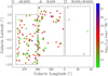 |
Fig. 1 SMGPS and X-ray counterpart positions in Galactic coordinates. The circles, triangles, and squares represent eRASS1, RASS, and combined RASS and eRASS1 detections positions respectively. The rectangular dashed lines are SMGPS footprints. |
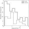 |
Fig. 2 Positional offsets between SMGPS radio detections and RASS/eRASS1 X-ray counterparts. |
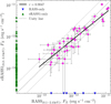 |
Fig. 3 Comparison of X-ray fluxes from the 41 RASS (0.1-2.4 keV band) and eRASS1 (0.2-2.3 keV band) common detections. The solid line shows the log-log fit to the matched sources, while the dashed line indicates the 1:1 (unity) relation. RASS-only and eRASS1-only detections are plotted along the respective axes. Factor-of-two dotted lines (y = 2x and y = x/2) illustrate typical potential variability between the surveys. |
4.2 Stellar populations
All sources were cross-matched with the SIMBAD archive (Wenger et al. 2000) to identify source populations. Our sample contains many spectral types across the HR diagram, including main-sequence, pre-main-sequence, and evolved stars (mainly of classical Cepheids and long-period variables). Also included are single and binary systems (see Fig. 4). K- and M-type stars dominate the population, many of which are identified as young stellar objects (YSOs). There are a handful of interacting binaries comprising the RS CVn, eclipsing, and spectroscopic binary systems. Radio and X-ray emission are expected from these populations, though different mechanisms drive the emission. For early-type stars, free-free (bremsstrahlung) emission from ionised stellar winds is the dominant mechanism producing radio emission. X-ray emission arises from shocks within the stellar winds of luminous OB-type systems (Guedel & Benz 1993; Güdel 2002, 2004). For late-type stars, the radio and X-ray activity is driven by gyrosynchrotron and coronal emission, respectively (Güdel 2002; Vedantham et al. 2022; Driessen et al. 2022).
The enhanced sensitivity of eRASS1 has significantly increased the number of known radio and X-ray emitting stars. While 41 stars are detected in both the RASS and eRASS1 samples, eRASS1 has enabled the additional detection of approximately three times as many stars, which were previously undetected in RASS.
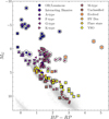 |
Fig. 4 Gaia colour-magnitude diagram for all 137 RASS and eRASS1 radio- and X-ray-emitting stars. The markers represent stellar classifications reported in (SIMBAD). The interacting binaries include the RS CVn, eclipsing, and spectroscopic binaries. Evolved stars comprise classical cepheids and long-period variables. The G-type, K-type, and M-type classifications are based on the Gaia astrophysical parameter catalogue (Gaia Collaboration 2023). The grey circles all represent Gaia DR3 sources within 100 pc of Earth, binned in uniform colour and magnitude. Large open circles represent the six detections in RASS that are not present in eRASS1, whereas the open squares show the 56 detections in eRASS1 that are absent in RASS and within 1kpc; the open hexagon markers show the 34 eRASS1 stars farther than 1 kpc away. |
4.3 Emission mechanisms
We calculated the radio brightness temperature, TB, of all the detections as explained in Section 3.2. We adopted the stellar radius provided by the Transiting Exoplanet Survey Satellite (TESS) input catalogue (TIC; Stassun et al. 2019; Paegert et al. 2021) for our sources. For sources with no radius value in the TIC, we searched the Gaia DR3 astrophysical parameters to obtain their radius. Also, we retrieved the Gaia distance estimates provided by Bailer-Jones et al. (2021). We followed a similar approach to Pritchard et al. (2021) in assuming that the emitting radius is three times the stellar radius (Re = 3R*).
The radio-brightness temperature, TB, versus the Gaia colour is given in Fig. 5, with the legend showing the spectral/stellar types. The radio-brightness temperatures vary among stars, which may reflect differences in coronal density, magnetic-field strength, and rotation rates. All our sources are at a brightness temperature of TB < 1012K, except for AX J1600.9-5142, which has a brightness temperature of TB = (4.8 ± 1.5) ∙ 1012 K. AX J1600.9-5142 is a well-known colliding-wind, double Wolf-Rayet binary, also known as Apep (del Palacio et al. 2023). An outlier at the lower end, with a TB of (8 ± 1) ∙ 106K, is HD 124831; it is a G3V-spectral-type binary system (Torres et al. 2006).
The majority of the sources have radio-brightness temperatures in the range of 109−1011 K. The eRASS1 sample includes sources brighter than 1010 K, unlike the RASS sample, whose maximum values are around 1010 K. The sensitivity of eRASS1 enabled the identification of fainter and more distant stellar counterparts, reaching distances of up to ~4500pc. Within the SMGPS/eRASS1 matched sample, 97 out of 131 sources lie within 1 kpc.
The radio-brightness temperature ranges obtained in this work are not uncommon for observations at a relatively low frequency of 1.3 GHz. For example, in Pritchard et al. (2021), all the stars are within the ~108−1011 K range, except for one late-type dwarf star with TB > 1012 K. Also, Ayanabha et al. (2024) showed that most of the VLASS detections within 500 pc at 3 GHz are within TB < 1012 K, except for late spectral types beyond M2.5. In this work, only AX J1600.9-5142 reached a brightness of > 1012 K, which is commonly adopted as the threshold distinguishing coherent from incoherent emission (Dulk 1985; Güdel 2002; Pritchard et al. 2021; Vedantham et al. 2022; Ayanabha et al. 2024). Hence, we conclude that all remaining stars exhibit incoherent radio emission predominantly produced by gyrosynchrotron emission.
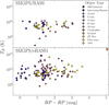 |
Fig. 5 Gaia (BP - RP) colour versus brightness temperature, TB, for SMGPS-X-ray matches with RASS and eRASS1 detections. Markers represent stellar classifications reported in SIMBAD. The interacting binaries include the RS CVn, eclipsing, and spectroscopic binaries. Evolved stars comprise classical cepheids and long-period variables. The G-type, K-type, and M-type classifications are based on the Gaia astrophysical parameter catalogue (Gaia Collaboration 2023). The vertical error bars show the propagated uncertainties from the flux measurements and distances. |
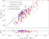 |
Fig. 6 X-ray luminosity as function of specific radio luminosity for SMGPS, RASS, and eRASS1 stars. The triangles and diamonds are detections from RASS and eRASS1, respectively. The black dots and grey crosses are the data from Guedel & Benz (1993); Benz & Guedel (1994) and Vedantham et al. (2022), respectively. The solid line in the top panel of the plot represents the Güdel-Benz fit from Williams et al. (2014). The grey circles and solid vertical lines in the top panel indicate sources detected by both RASS and eRASS1. For each source, the vertical line connects the RASS and eRASS1 measurements, illustrating the level of X-ray variability. The bottom panel shows the residuals of the data from the GBR fit. The error bars in both panels indicate the propagated uncertainties in the measured fluxes and geometric distances for each source. |
4.4 Radio-X-ray-luminosity relationship
We investigated the GBR for our sources by calculating the radio and X-ray luminosities using the SMGPS radio fluxes and X-ray fluxes from both RASS and eRASS1, and geometric distance estimates information from Bailer-Jones et al. (2021). The radio and X-ray luminosity parameter space is shown in Fig. 6, which also features the sources used to derive the canonical GBR from Guedel & Benz (1993) and Benz & Guedel (1994), as well as the LOFAR sources from Vedantham et al. (2022). To enable a consistent comparison across samples, we note that the Guedel & Benz (1993); Benz & Guedel (1994) and Vedantham et al. (2022), and our sample X-ray fluxes were derived using thermal coronal spectrum (e.g. Raymond-Smith, APEC) models appropriate for active stellar coronae (Benz & Guedel 1994; Schmitt et al. 1995; Fleming et al. 1995). For the radio data, the samples differ in observing frequency; the GBR used 5-9 GHz measurements (Benz & Guedel 1994), the SMGPS luminosities are based on 1.3 GHz flux densities, and the Vedantham et al. (2022) sample used LOFAR observations at 144 MHz. Active stellar radio spectra are often flat or only mildly inverted in the gigahertz regime (e.g. Güdel 2002), while low-frequency (100200 MHz) emission is dominated by non-thermal processes such as gyrosynchrotron or coherent bursts and still traces magnetic activity (Zic et al. 2019; Callingham et al. 2021). These frequency differences may introduce some systematic offsets or scatter. Still, the comparison remains appropriate for assessing the overall form of the radio-X-ray correlation as the GBR is observed to hold over a range of frequencies from 200 MHz to 9 GHz. The solid line in Fig. 6 shows the canonical GBR fit parametrised by Williams et al. (2014). The RASS sources are scattered around the GBR fit with a dispersion of ~0.53 dex, whereas eRASS1 sources are scattered around the fit with a slightly larger dispersion of 0.57 dex. Overall, our samples are distributed along the GBR fit, but with a higher concentration of sources below the GBR fit line. The bottom panel plot in Fig. 6 shows the residuals from the GBR plotted against Lν,R for both RASS and eRASS1 sources.
In our sample, the canonical GBR appears to represent the upper envelope of the LX-Lν,R correlation. Stars with LX > 1029 erg s−1 are broadly consistent with the GBR, although they exhibit a spread of more than 2 dex in Lν,R . There is also a notable absence of stars with LX between 1028 and 1029 erg s−1 lying on the GBR; the detected objects in this regime show systematically higher Lν,R than expected. Their X-ray luminosities fall within the range expected for coronally active stars, so the deviation cannot be explained by unusually weak X-ray emission. A plausible explanation is the radio sensitivity limit, whereby only stars observed during flaring or enhanced non-thermal states exceed the radio detection threshold, while quiescent emission remains undetected. However, we note that the small sky coverage of the survey (~ 1.2%) may also contribute to the observed distribution if such radio-bright states or objects are intrinsically rare.
Specific radio luminosities above the canonical GBR are well established for several stellar regimes and can arise from sensitivity-driven selection effects in the radio band. For low-luminosity late-M and ultra-cool dwarfs, numerous studies have shown that radio emission is systematically over-luminous by several orders of magnitude, because only flaring or strongly magnetically active sources exceed current radiodetection thresholds for this population (Berger 2006; Berger et al. 2010; Williams et al. 2014; Villadsen & Hallinan 2019). Likewise, recent surveys of solar-type G and K stars show that most radio detections correspond to short-duration flares or enhanced non-thermal activity, while the quiescent levels remain below the instrumental sensitivity (Yiu et al. 2024; Driessen et al. 2024). These sensitivity effects can therefore broaden the observed LX-Lν,R distribution and shift the apparent offset to higher luminosities when sampling more distant or intrinsically brighter stellar populations. In the context of our sample, this implies that the excess radio luminosities we observe relative to the classical GBR may reflect the detection of only the most radio-active or magnetically active sources within the SMGPS survey, rather than a fundamental deviation in the underlying coronal physics.
4.4.1 Power-law correlations
To assess whether our radio-X-ray-selected sample is consistent with the GBR, we fitted a power-law function in logarithmic space to the SMGPS specific luminosities and X-ray luminosities derived from RASS and eRASS1 counterparts, as shown in Fig. 7. Parameters of the best fits are given in Table 1. The RASS-SMGPS correlation shows a Kendall τ (Kendall 1938) correlation coefficient of τ = 0.576 with a p value of 1.11 ∙ 10−8, and the eRASS1-SMGPS correlation results in τ = 0.626 and a p value of 1.20 ∙ 10−29.
The eRASS1-derived slope of the LX-Lν,R relation (0.68 ± 0.04) is in close agreement with the Williams et al. (2014) canonical GBR exponent of 0.73 (see Eq. (1)), indicating that the fundamental scaling between coronal X-ray and non-thermal radio emission remains valid for our sample. The fitted normalisation is within 2σ of the canonical relation with no quoted uncertainty. On the other hand, the RASS relation yields a slightly steeper slope (0.8 ± 0.1), but with a significantly larger scatter in the LX-LR plane. The broad dispersion observed for RASS may reflect a combination of factors, including ROSATs lower sensitivity level, which may bias detections towards variable or X-ray-luminous subsets of sources.
Generally, both RASS and eRASS1 have roughly the same vertical spread across the GBR. However, eRASS1 allows for the detection of objects approximately one order of magnitude more luminous than the brightest RASS source in our sample, with the SMGPS radio luminosity being three orders of magnitude brighter than that of the RASS samples. Comparing our SMGPS samples to GBR, some GBR sources appear less luminous in both the radio and X-rays. This can be attributed to the flux limit of our sample. In addition, two stars (AX J1600.9-5142 and HD 93129A) show excessive radio luminosities beyond 1020 erg s−1 Hz−1. Both systems are very-early-type interacting binaries (del Palacio et al. 2023; Benaglia et al. 2025).
By contrast, eROSITA’s improved sensitivity provides a more complete sampling of coronal X-ray emission, especially among fainter sources that were below the detection limit of ROSAT. This yields a tighter LX-Lν,R correlation for the coronal population. Although the eRASS1 sample extends to larger distances and contains a broad mix of stellar types, the tighter relation arises because eROSITA detects the full range of coronal luminosities rather than only the brightest or most variable objects. Non-coronal emitters (e.g. massive OB stars and interacting binaries, whose X-rays are wind driven) do not dominate the fitted correlation (Freund et al. 2024), ensuring that the observed trend reflects the intrinsic behaviour of magnetically active coronal sources rather than contamination from unrelated emission mechanisms.
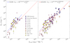 |
Fig. 7 X-ray luminosity as function of specific radio luminosity for the SMGPS-RASS (left) and eRASS1 (right) sources. In each panel, the solid line shows the fit to that dataset, while the dashed line shows the fit obtained from the other dataset. The markers show object/spectral-type information obtained from either SIMBAD or Gaia Collaboration (2023) Gaia DR3 astrophysical parameters. |
Power-law fits to luminosity relationships of RASS and eRASS1 samples.
4.4.2 Implications for coronal emission and stellar populations
Our findings highlight the importance of sample selection and instrument sensitivity in characterising correlations such as the GBR. While both RASS and eRASS1 samples show broadly consistent scaling behaviour, the tighter relation obtained with eRASS1 supports its robustness across a more diverse sample with higher statistics.
4.5 Comparison with optical luminosities
Using the identified samples, we examine correlations of Lν,R and LX with the bolometric1 luminosity, Lbol. We fitted the correlations with a power-law function and show the relationships for all cases in Table 1 and Figs 8 and 9. In Fig. 8, both the RASS and eRASS1 samples show no obvious correlation along the best-fit relation. However, for eRASS1, we see two clusters of populations: one below Lbol ~ 1037 ergs−1 dominated by coronally active stars; and above it, the massive high-luminosity sources whose radio-emission origins are driven by thermal wind. In Fig. 9, the LX-Lbol relation shows a clear correlation for the RASS sample, with sources broadly scattered around the best-fit line. In contrast, the eRASS1 distribution becomes highly irregular at higher bolometric luminosities, showing no clear correlation. When restricting the comparison to coronal sources only, the RASS-derived fit provides a better description of the coronal subset within eRASS1, whereas the non-coronal eRASS1 objects (principally OB and evolved stars) deviate strongly from any LX-Lbol trend. The broader diversity seen in Figs. 8 and 9 is revealed only by the higher sensitivity of eRASS1, where RASS does not reach into the domain where the correlation between LX versus Lbol and Lν,R versus Lbol breaks down.
Given that the early-type stars detected in eRASS1 do not conform well with the LX vs Lbol correlation, we excluded the early-type samples comprising OB-luminous, A-type, F-type, and intermediate binaries from further analysis. Specifically, we focused on fitting the X-ray luminosity as a function of bolometric luminosity, Lbol, for the corona-dominated later type stars in contrast to the full-sample fits presented in Table 1 ; this was done to constrain the coronal emission component and obtain a more meaningful fit. We achieved a linear fit of  (see Fig. 10), indicating that the X-ray luminosity, LX, scales with bolometric luminosity, Lbol, with an exponent of 0.76; this indicates that the growth of LX with Lbol is shallower than a one-to-one relation. In addition, most stars in this sample have log(LX/Lbol) ≈ −3, with a few reaching values as low as −7. The clustering around −3 is consistent with the coronal saturation limit observed in rapidly rotating, magnetically active stars, while the lower ratios likely represent less active and older coronae. This sample separation in Fig. 10, where log(LX/Lbol) ≥ −5 represents coronal sources and log(LX/Lbol) < -5 represents non-coronal (wind-driven) emitters, is not a universal boundary, as many coronal stars, including the Sun with log(LX/Lbol) ≈ −6, fall below this threshold. The apparent separation arises because eRASS1 preferentially detects the more luminous coronal sources (near the saturation limit log(LX/Lbol)~ −3), while lower activity coronae can only be observed within a small local volume. The slope below unity implies that as Lbol increases, the relative X-ray output (LX/Lbol) decreases. This trend is more consistent with reduced dynamo efficiency in more luminous, more slowly rotating stars. This behaviour is well established in studies of coronal X-ray scaling (e.g. Güdel (2004) and Reiners et al. (2014) and supports the interpretation that late-type stars in our sample are dominated by magnetically heated stellar coronae.
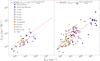 |
Fig. 8 Specific radio luminosity, Lν,R, as a function of bolometric luminosity, Lbol, for the SMGPS-RASS, eRASS1 sources. The solid and dashed lines, and markers are the same as in Fig. 7. The blue and red lines in both panels are the power-law fit for RASS and eRASS1, respectively. |
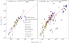 |
Fig. 9 X-ray luminosity, LX as a function of bolometric luminosity, Lbol for the SMGPS-RASS, eRASS1 sources. The solid and dashed lines, and markers are the same as in Fig. 7. The blue and red lines in both panels are the powerlaw fit for RASS and eRASS1, respectively. |
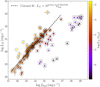 |
Fig. 10 X-ray luminosity, LX, as a function of bolometric luminosity, Lbol, for the eRASS1-detected stars colour coded by the log(LX/Lbol). Circles and triangles indicate sources with log(LX/Lbol) ≥ −5 and log(LX/Lbol) < −5, respectively. In our flux-limited sample, the former group is dominated by coronally active stars, while the latter is consistent with non-coronal (wind-driven) emitters. The dashed line represents the linear fit in log-log space for all the stars (indicated with large open circles), excluding OB-luminous, A-type, F-type and intermediate binaries, which are indicated with open squares. |
5 Conclusions
We identified 137 radio and X-ray emitting stars obtained by cross-correlating the SARAO MeerKAT Galactic-plane compact source catalogue with soft X-ray detections from RASS and eRASS1. The radio-brightness temperature of almost all the stars in the sample is ≤ 1012 K, indicating that the radio detections at 1.3 GHz are consistent with incoherent gyrosynchrotron emission from mildly relativistic electrons in stellar coronae, as observed in other magnetically active stars. We find that the radio and X-ray luminosities of our sample are correlated; however, the GBR does not strictly hold for all sources. Instead, it appears to trace the upper envelope of the LX-Lν,R distribution, suggesting that while some stars approach the canonical relation, many lie below it. When compared to the canonical GBR, the majority of sources observed at 1.3 GHz appear over-luminous in the radio relative to the canonical GBR. This offset is primarily driven by enhanced radio luminosities rather than suppressed X-ray emission, which is consistent with the broader radio luminosity distribution sampled by the eRASS1 population. Our power-law fits to the Lx-Lν,R relation yield slopes consistent with those of the canonical GBR for both RASS and eRASS1, indicating that the relative scaling between the coronal soft X-ray and nonthermal radio emission is similar for our population, but the normalisation differs. Additionally, the eRASS1 sources reveal a more diverse population, including massive/luminous sources, compared to that based on RASS. We derived scaling relations for specific radio and bolometric luminosities (Lν,R versus Lbol) and X-ray and bolometric luminosities (LX versus Lbol). These relations reveal trends in our data that may reflect underlying stellar properties, such as rotation and spectral type, thanks to eRASS1 data. In examining the LX-Lbol relation, we found that the early-type stars do not follow the same trend as the late-type stars. By fitting only the late-type stars, we obtained a robust power-law fit for the X-ray-versus-bolometric luminosity with most stars showing log(LX/Lbol)~ −3, which is consistent with coronal saturation levels.
Looking forward, future eROSITA all-sky survey data releases (DR2 and DR3) will provide deeper X-ray coverage and improved statistics for stellar samples, enabling more robust population studies. At the same time, next-generation radio facilities, most particularly the Square Kilometre Array (SKA), will deliver unprecedented sensitivity levels. Together, the datasets will provide powerful synergies for probing stellar magnetic activity and refining our understanding of radio- and X-ray-emitting stars in our Galaxy.
Data availability
Information about the SARAO Galactic Plane Survey can be found in Goedhart et al. (2024) and the compact source catalogue in Mutale et al. (2026). The coronal X-ray data from ROSAT and eROSITA eRASS1 are available in Freund et al. (2022) and Freund et al. (2024), respectively. The Gaia DR3 data used in this work are available in the CDS Vizier database; the details can be found in Gaia Collaboration (2023). The radio-X-ray star catalogue from this work is available at the CDS via https://cdsarc.cds.unistra.fr/viz-bin/cat/J/A+A/707/A193 and the details of the column description are listed in Table A.1.
Acknowledgements
The authors would like to thank H.K. Vedantham for sharing his code and data for making the radio-X-ray luminosity plot. This work is based on research fully supported by the National Research Foundation’s (NRF) South African Astronomical Observatory (SAAO) PhD Prize Scholarship. P.J.G. and O.D.E. are (partly) supported by the NRF SARChI grant 111692. D.A.H.B. acknowledges research support by the National Research Foundation. J.R. acknowledges support from DLR under 50QR2505. The MeerKAT telescope is operated by the South African Radio Astronomy Observatory, which is a facility of the National Research Foundation, an agency of the Department of Science and Innovation. We acknowledge the use of the ilifu cloud computing facility - www.ilifu.ac.za, a partnership between the University of Cape Town, the University of the Western Cape, Stellenbosch University, Sol Plaatje University and the Cape Peninsula University of Technology. The ilifu facility is supported by contributions from the Inter-University Institute for Data Intensive Astronomy (IDIA - a partnership between the University of Cape Town, the University of Pretoria and the University of the Western Cape), the Computational Biology division at UCT and the Data Intensive Research Initiative of South Africa (DIRISA). This work has made use of data from the European Space Agency (ESA) mission Gaia, processed by the Gaia Data Processing and Analysis Consortium (DPAC). Funding for the DPAC has been provided by national institutions, in particular the institutions participating in the Gaia Multilateral Agreement. This research has made use of the VizieR catalogue access tool, CDS, Strasbourg, France (DOI:1®.26093/cds/vizier). The original description of the VizieR service was published in 2000, A&AS 143, 23. This work is based on data from eROSITA, the soft X-ray instrument aboard SRG, a joint Russian-German science mission supported by the Russian Space Agency (Roskosmos), in the interests of the Russian Academy of Sciences represented by its Space Research Institute (IKI), and the Deutsches Zentrum für Luft- und Raumfahrt (DLR). The SRG spacecraft was built by Lavochkin Association (NPOL) and its subcontractors, and is operated by NPOL with support from the Max Planck Institute for Extraterrestrial Physics (MPE). The development and construction of the eROSITA X-ray instrument was led by MPE, with contributions from the Dr. Karl Remeis Observatory Bamberg & ECAP (FAU Erlangen-Nuernberg), the University of Hamburg Observatory, the Leibniz Institute for Astrophysics Potsdam (AIP), and the Institute for Astronomy and Astrophysics of the University of Tübingen, with the support of DLR and the Max Planck Society. The Argelander Institute for Astronomy of the University of Bonn and the Ludwig Maximilians Universität Munich also participated in the science preparation for eROSITA. The eROSITA data shown here were processed using the eSASS software system developed by the German eROSITA consortium. This research used ASTROPY, a community-developed core Python package for Astronomy (Astropy Collaboration 2013; Astropy Collaboration et al. 2018). We also use NUMPY (Harris et al. 2020), SCIPY (Virtanen et al. 2020), PANDAS (pandas development team 2020), and MATPLOTLIB (Hunter 2007). This research has used the SIMBAD database, operated at CDS, Strasbourg, France.
References
- Astropy Collaboration (Robitaille, T. P., et al.) 2013, A&A, 558, A33 [NASA ADS] [CrossRef] [EDP Sciences] [Google Scholar]
- Astropy Collaboration (Price-Whelan, A. M., et al.) 2018, AJ, 156, 123 [Google Scholar]
- Ayanabha, D., Narang, M., Puravankara, M., et al. 2024, AJ, 168, 288 [Google Scholar]
- Bailer-Jones, C. A. L., Rybizki, J., Fouesneau, M., Demleitner, M., & Andrae, R. 2021, AJ, 161, 147 [Google Scholar]
- Benaglia, P., del Palacio, S., Saponara, J., et al. 2025, A&A, 698, A23 [NASA ADS] [CrossRef] [EDP Sciences] [Google Scholar]
- Benz, A. O., & Guedel, M. 1994, A&A, 285, 621 [NASA ADS] [Google Scholar]
- Berger, E. 2006, ApJ, 648, 629 [NASA ADS] [CrossRef] [Google Scholar]
- Berger, E., Basri, G., Fleming, T. A., et al. 2010, ApJ, 709, 332 [Google Scholar]
- Boller, T., Freyberg, M. J., Trümper, J., et al. 2016, A&A, 588, A103 [NASA ADS] [CrossRef] [EDP Sciences] [Google Scholar]
- Callingham, J. R., Vedantham, H. K., Shimwell, T. W., et al. 2021, NatAs, 5, 1233 [NASA ADS] [Google Scholar]
- del Palacio, S., García, F., De Becker, M., et al. 2023, A&A, 672, A109 [NASA ADS] [CrossRef] [EDP Sciences] [Google Scholar]
- Díaz-Márquez, E., Grau, R., Busquet, G., et al. 2024, A&A, 682, A180 [NASA ADS] [CrossRef] [EDP Sciences] [Google Scholar]
- Drake, S. A., Abbott, D. C., Bastian, T. S., et al. 1987, ApJ, 322, 902 [NASA ADS] [CrossRef] [Google Scholar]
- Driessen, L. N., Williams, D. R. A., McDonald, I., et al. 2022, MNRAS, 510, 1083 [Google Scholar]
- Driessen, L. N., Pritchard, J., Murphy, T., et al. 2024, PASA, 41, e084 [NASA ADS] [CrossRef] [Google Scholar]
- Dulk, G. A. 1985, ARA&A, 23, 169 [Google Scholar]
- Egbo, O. D., Buckley, D. A. H., Groot, P. J., et al. 2025, MNRAS, 540, 2685 [Google Scholar]
- Fleming, T A., Molendi, S., Maccacaro, T., & Wolter, A. 1995, ApJS, 99, 701 [Google Scholar]
- Forbrich, J., Wolk, S. J., Güdel, M., et al. 2011, in Astronomical Society of the Pacific Conference Series, 448, 16th Cambridge Workshop on Cool Stars, Stellar Systems, and the Sun, eds. C. Johns-Krull, M. K. Browning, & A. A. West, 455 [Google Scholar]
- Franciosini, E., & Chiuderi Drago, F. 1995, A&A, 297, 535 [Google Scholar]
- Freund, S., Czesla, S., Robrade, J., Schneider, P. C., & Schmitt, J. H. M. M. 2022, A&A, 664, A105 [NASA ADS] [CrossRef] [EDP Sciences] [Google Scholar]
- Freund, S., Czesla, S., Predehl, P., et al. 2024, A&A, 684, A121 [NASA ADS] [CrossRef] [EDP Sciences] [Google Scholar]
- Gaia Collaboration (Brown, A. G. A., et al.) 2021, A&A, 649, A1 [NASA ADS] [CrossRef] [EDP Sciences] [Google Scholar]
- Gaia Collaboration (Vallenari, A., et al.) 2023, A&A, 674, A1 [NASA ADS] [CrossRef] [EDP Sciences] [Google Scholar]
- Goedhart, S., Cotton, W. D., Camilo, F., et al. 2024, MNRAS, 531, 649 [CrossRef] [Google Scholar]
- Gordon, Y. A., Boyce, M. M., O’Dea, C. P., et al. 2021, ApJS, 255, 30 [NASA ADS] [CrossRef] [Google Scholar]
- Güdel, M. 2002, ARA&A, 40, 217 [Google Scholar]
- Güdel, M. 2004, A&ARv, 12, 71 [CrossRef] [Google Scholar]
- Guedel, M., & Benz, A. O. 1993, ApJ, 405, L63 [NASA ADS] [CrossRef] [Google Scholar]
- Hancock, P. J., Trott, C. M., & Hurley-Walker, N. 2018, Source Finding in the Era of the SKA (Precursors): Aegean 2.0 [Google Scholar]
- Harris, C. R., Millman, K. J., van der Walt, S. J., et al. 2020, Nature, 585, 357 [NASA ADS] [CrossRef] [Google Scholar]
- Hjellming, R. M. 1988, in Galactic and Extragalactic Radio Astronomy, eds. K. I. Kellermann & G. L. Verschuur, 381 [Google Scholar]
- Hunter, J. D. 2007, Comput. Sci. Eng., 9, 90 [NASA ADS] [CrossRef] [Google Scholar]
- Kendall, M. G. 1938, Biometrika, 30, 81 [Google Scholar]
- Lacy, M., Baum, S. A., Chandler, C. J., et al. 2020, PASP, 132, 035001 [Google Scholar]
- Launhardt, R., Loinard, L., Dzib, S. A., et al. 2022, ApJ, 931, 43 [NASA ADS] [CrossRef] [Google Scholar]
- Linsky, J. L. 1996, in Astronomical Society of the Pacific Conference Series, 93, Radio Emission from the Stars and the Sun, eds. A. R. Taylor, & J. M. Paredes, 439 [Google Scholar]
- Merloni, A., Lamer, G., Liu, T., et al. 2024, A&A, 682, A34 [NASA ADS] [CrossRef] [EDP Sciences] [Google Scholar]
- Morris, D. H., Mutel, R. L., & Su, B. 1990, ApJ, 362, 299 [Google Scholar]
- Mutale, M., Thompson, M. A., Williams, G. M., et al. 2026, MNRAS, 546, staf1849 [Google Scholar]
- Nandy, D. 2004, SoPh, 224, 161 [Google Scholar]
- Noyes, R. W., Hartmann, L. W., Baliunas, S. L., Duncan, D. K., & Vaughan, A. H. 1984, ApJ, 279, 763 [Google Scholar]
- Ochsenbein, F., Bauer, P., & Marcout, J. 2000, A&AS, 143, 23 [Google Scholar]
- Paegert, M., Stassun, K. G., Collins, K. A., et al. 2021, arXiv [arXiv:2108.04778] [Google Scholar]
- pandas development team, T. 2020, pandas-dev/pandas: Pandas [Google Scholar]
- Pecaut, M. J., & Mamajek, E. E. 2013, ApJS, 208, 9 [Google Scholar]
- Predehl, P., Andritschke, R., Arefiev, V., et al. 2021, A&A, 647, A1 [EDP Sciences] [Google Scholar]
- Pritchard, J., Murphy, T., Zic, A., et al. 2021, MNRAS, 502, 5438 [NASA ADS] [CrossRef] [Google Scholar]
- Reiners, A., Schüssler, M., & Passegger, V. M. 2014, ApJ, 794, 144 [Google Scholar]
- Schmitt, J. H. M. M., Fleming, T. A., & Giampapa, M. S. 1995, ApJ, 450, 392 [Google Scholar]
- Schneider, P. C., Freund, S., Czesla, S., et al. 2022, A&A, 661, A6 [NASA ADS] [CrossRef] [EDP Sciences] [Google Scholar]
- Schrijver, C. J. 1985, SSRv, 40, 3 [Google Scholar]
- Schrijver, C. J., Mewe, R., & Walter, F. M. 1984, A&A, 138, 258 [NASA ADS] [Google Scholar]
- Seaquist, E. R. 1993, RPPh, 56, 1145 [Google Scholar]
- Shimwell, T. W., Röttgering, H. J. A., Best, P. N., et al. 2017, A&A, 598, A104 [NASA ADS] [CrossRef] [EDP Sciences] [Google Scholar]
- Shimwell, T. W., Tasse, C., Hardcastle, M. J., et al. 2019, A&A, 622, A1 [NASA ADS] [CrossRef] [EDP Sciences] [Google Scholar]
- Skumanich, A., Smythe, C., & Frazier, E. N. 1975, ApJ, 200, 747 [Google Scholar]
- Stassun, K. G., Oelkers, R. J., Paegert, M., et al. 2019, AJ, 158, 138 [Google Scholar]
- Testa, P. 2010a, SSRv, 157, 37 [Google Scholar]
- Testa, P. 2010b, PNAS, 107, 7158 [NASA ADS] [CrossRef] [Google Scholar]
- Testa, P., Saar, S. H., & Drake, J. J. 2015, RSPTA, 373, 20140259 [Google Scholar]
- Toet, S. E. B., Vedantham, H. K., Callingham, J. R., et al. 2021, A&A, 654, A21 [NASA ADS] [CrossRef] [EDP Sciences] [Google Scholar]
- Torres, C. A. O., Quast, G. R., da Silva, L., et al. 2006, A&A, 460, 695 [NASA ADS] [CrossRef] [EDP Sciences] [Google Scholar]
- Trigilio, C., Umana, G., Cavallaro, F., et al. 2018, MNRAS, 481, 217 [NASA ADS] [CrossRef] [Google Scholar]
- Truemper, J. 1982, AdSpR, 2, 241 [Google Scholar]
- van Haarlem, M. P., Wise, M. W., Gunst, A. W., et al. 2013, A&A, 556, A2 [NASA ADS] [CrossRef] [EDP Sciences] [Google Scholar]
- Vedantham, H. K. 2020, A&A, 639, L7 [NASA ADS] [CrossRef] [EDP Sciences] [Google Scholar]
- Vedantham, H. K., Callingham, J. R., Shimwell, T. W., et al. 2022, ApJ, 926, L30 [NASA ADS] [CrossRef] [Google Scholar]
- Villadsen, J., & Hallinan, G. 2019, ApJ, 871, 214 [Google Scholar]
- Virtanen, P., Gommers, R., Oliphant, T. E., et al. 2020, Nat. Methods, 17, 261 [Google Scholar]
- Voges, W., Aschenbach, B., Boller, T., et al. 1999, A&A, 349, 389 [NASA ADS] [Google Scholar]
- Wenger, M., Ochsenbein, F., Egret, D., et al. 2000, A&AS, 143, 9 [NASA ADS] [Google Scholar]
- Williams, P. K. G., Cook, B. A., & Berger, E. 2014, ApJ, 785, 9 [Google Scholar]
- Yiu, T. W. H., Vedantham, H. K., Callingham, J. R., & Günther, M. N. 2024, A&A, 684, A3 [NASA ADS] [CrossRef] [EDP Sciences] [Google Scholar]
- Zhuleku, J., Warnecke, J., & Peter, H. 2020, A&A, 640, A119 [NASA ADS] [CrossRef] [EDP Sciences] [Google Scholar]
- Zic, A., Stewart, A., Lenc, E., et al. 2019, MNRAS, 488, 559 [Google Scholar]
We computed Lbol from the de-reddened Gaia G-band magnitude, applying bolometric corrections based on spectral classes from a table based on Pecaut & Mamajek (2013), which is regularly updated at http://www.pas.rochester.edu/~emamajek/EEM_dwarf_UBVIJHK_colors_Teff.txt (current version 2022.04.16).
Appendix A Column description
Column definitions with units and descriptions.
All Tables
All Figures
|
Fig. 1 SMGPS and X-ray counterpart positions in Galactic coordinates. The circles, triangles, and squares represent eRASS1, RASS, and combined RASS and eRASS1 detections positions respectively. The rectangular dashed lines are SMGPS footprints. |
| In the text | |
|
Fig. 2 Positional offsets between SMGPS radio detections and RASS/eRASS1 X-ray counterparts. |
| In the text | |
|
Fig. 3 Comparison of X-ray fluxes from the 41 RASS (0.1-2.4 keV band) and eRASS1 (0.2-2.3 keV band) common detections. The solid line shows the log-log fit to the matched sources, while the dashed line indicates the 1:1 (unity) relation. RASS-only and eRASS1-only detections are plotted along the respective axes. Factor-of-two dotted lines (y = 2x and y = x/2) illustrate typical potential variability between the surveys. |
| In the text | |
|
Fig. 4 Gaia colour-magnitude diagram for all 137 RASS and eRASS1 radio- and X-ray-emitting stars. The markers represent stellar classifications reported in (SIMBAD). The interacting binaries include the RS CVn, eclipsing, and spectroscopic binaries. Evolved stars comprise classical cepheids and long-period variables. The G-type, K-type, and M-type classifications are based on the Gaia astrophysical parameter catalogue (Gaia Collaboration 2023). The grey circles all represent Gaia DR3 sources within 100 pc of Earth, binned in uniform colour and magnitude. Large open circles represent the six detections in RASS that are not present in eRASS1, whereas the open squares show the 56 detections in eRASS1 that are absent in RASS and within 1kpc; the open hexagon markers show the 34 eRASS1 stars farther than 1 kpc away. |
| In the text | |
|
Fig. 5 Gaia (BP - RP) colour versus brightness temperature, TB, for SMGPS-X-ray matches with RASS and eRASS1 detections. Markers represent stellar classifications reported in SIMBAD. The interacting binaries include the RS CVn, eclipsing, and spectroscopic binaries. Evolved stars comprise classical cepheids and long-period variables. The G-type, K-type, and M-type classifications are based on the Gaia astrophysical parameter catalogue (Gaia Collaboration 2023). The vertical error bars show the propagated uncertainties from the flux measurements and distances. |
| In the text | |
|
Fig. 6 X-ray luminosity as function of specific radio luminosity for SMGPS, RASS, and eRASS1 stars. The triangles and diamonds are detections from RASS and eRASS1, respectively. The black dots and grey crosses are the data from Guedel & Benz (1993); Benz & Guedel (1994) and Vedantham et al. (2022), respectively. The solid line in the top panel of the plot represents the Güdel-Benz fit from Williams et al. (2014). The grey circles and solid vertical lines in the top panel indicate sources detected by both RASS and eRASS1. For each source, the vertical line connects the RASS and eRASS1 measurements, illustrating the level of X-ray variability. The bottom panel shows the residuals of the data from the GBR fit. The error bars in both panels indicate the propagated uncertainties in the measured fluxes and geometric distances for each source. |
| In the text | |
|
Fig. 7 X-ray luminosity as function of specific radio luminosity for the SMGPS-RASS (left) and eRASS1 (right) sources. In each panel, the solid line shows the fit to that dataset, while the dashed line shows the fit obtained from the other dataset. The markers show object/spectral-type information obtained from either SIMBAD or Gaia Collaboration (2023) Gaia DR3 astrophysical parameters. |
| In the text | |
|
Fig. 8 Specific radio luminosity, Lν,R, as a function of bolometric luminosity, Lbol, for the SMGPS-RASS, eRASS1 sources. The solid and dashed lines, and markers are the same as in Fig. 7. The blue and red lines in both panels are the power-law fit for RASS and eRASS1, respectively. |
| In the text | |
|
Fig. 9 X-ray luminosity, LX as a function of bolometric luminosity, Lbol for the SMGPS-RASS, eRASS1 sources. The solid and dashed lines, and markers are the same as in Fig. 7. The blue and red lines in both panels are the powerlaw fit for RASS and eRASS1, respectively. |
| In the text | |
|
Fig. 10 X-ray luminosity, LX, as a function of bolometric luminosity, Lbol, for the eRASS1-detected stars colour coded by the log(LX/Lbol). Circles and triangles indicate sources with log(LX/Lbol) ≥ −5 and log(LX/Lbol) < −5, respectively. In our flux-limited sample, the former group is dominated by coronally active stars, while the latter is consistent with non-coronal (wind-driven) emitters. The dashed line represents the linear fit in log-log space for all the stars (indicated with large open circles), excluding OB-luminous, A-type, F-type and intermediate binaries, which are indicated with open squares. |
| In the text | |
Current usage metrics show cumulative count of Article Views (full-text article views including HTML views, PDF and ePub downloads, according to the available data) and Abstracts Views on Vision4Press platform.
Data correspond to usage on the plateform after 2015. The current usage metrics is available 48-96 hours after online publication and is updated daily on week days.
Initial download of the metrics may take a while.